
MMT – Multipoint Measurement Tool#
MMT - Tutorial#
Overview#
The MMT Multipoint Measurement Tool is used to determine the linear electrical and mechanical parameters (Thiele‑Small parameters) of electro-dynamical transducers. In contrast to the LPM – Linear Parameter Measurement, the MMT can use multiple measurements taken on different points of the membrane, to cope with rocking modes or other vibration effects. In addition, measurements taken in vacuum, air and with attached load (e.g., an enclosure) can be used. The resulting separated parameters are calculated and displayed, and aid the evaluation of the air or enclosure impact.
What is the Goal of This Tutorial?#
This tutorial makes you familiar with the MMT module.
The tutorial is divided into three parts:
In the first section, Viewing MMT Results, we will show you how to view MMT results already stored in the web example database.
The next part of the tutorial, Performing a new MMT, provides a step-by-step recipe to measure the electrical and mechanical driver parameters using the MMT.
In the final section, Customizing MMT, we discuss modifications of the setup parameters to use more powerful features and to improve the performance of the measurement.
In the chapter MMT - Reference you will find more information on the basics of the linear model used as well as a detailed description of the result windows and the configuration of the property pages.
In the last section, you will find information on possible problems, malfunctions and troubleshooting.
Note
It is highly recommended to take a look at the LPM Linear Parameter Measurement manual first. The MMT acts as an advanced post-processing tool, the necessary measurements are performed within the LPM module.
Viewing MMT Results (Part 1)#
Example data used in this manual is stored in the Web Example database. If not downloaded already, get it from the latest R&D release <https://www.klippel.de/go/current-rnd-release> and open the web-based database.
See also
View Results for general information on how to download this database, open and view results in dB-Lab.
Open and select the operation:
Please refer to the dBLab manual section for navigating within, or selecting, databases.
After double clicking the operation, the default result windows will be opened.
Table Linear Parameters#
The result window shows the electrical and mechanical parameters of the linear driver model, the derived parameters (resonance frequency, loss factors etc.) and the parameter of the suspension creep factor that are determined by the MMT.
The most important results are:
\(R_{\text{e}}\): Electrical voice coil resistance at DC.
\(L_{\text{e}}\): Frequency independent part of the voice coil inductance.
\(f_{\text{s}}\): Driver resonance frequency.
\(M_{\text{ms}}\): Mechanical mass of driver diaphragm assembly including air load and voice coil.
\(Bl\): Effective force factor (\(Bl\)-product).
H(f) Magnitude#
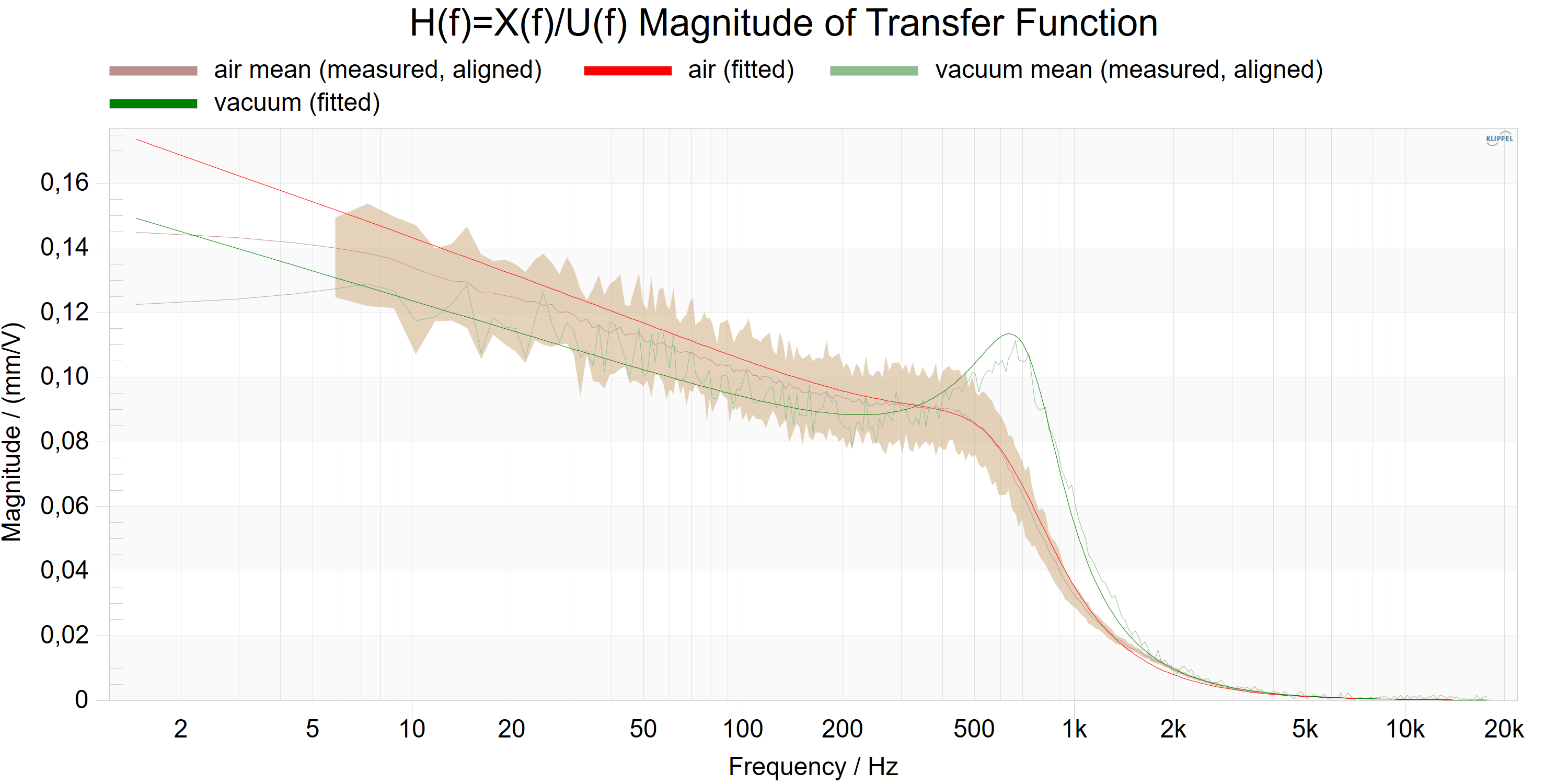
The result window shows the magnitude of the measured and estimated transfer functions \(H_{x}(f) = \frac{X(f)}{U(f)}\) between the voice coil displacement \(X(f)\) and the terminal voltage \(U(f)\). The measured curves are the ratio of the acquired spectra \(X(f)\) and \(U(f)\) , while the fitted curve is the transfer function based on the linear model, using the identified electrical and mechanical parameters as well as the creep parameter. Since multiple air measurements were used, a mean curve of all measurements as well as an area marking maximum and minimum points is displayed. In addition, a vacuum measurement is available, outlining the impact of the air on the laser measurement (higher resonance frequency / quality factor without air impact).
The creep effect models the low frequency behavior of the suspension system of a loudspeaker. The stiffness is not constant over frequency but decreases for very low frequencies. For more information, see the reference / linear modeling of MMT. In contrary to the LPM, no curve shows the fitting without creep effect.
Z(f) Impedance Magnitude#
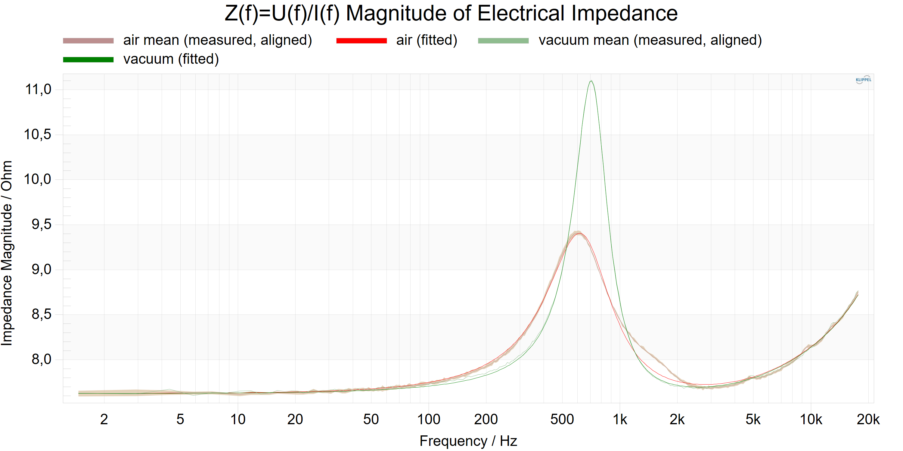
The result window shows the magnitude of the measured and estimated impedance \(Z(f) = \frac{U(f)}{I(f)}\) where \(U(f)\) is the terminal voltage and \(I(f)\) is the current. The measured curves are the ratio of the measured spectra \(U(f)\) and \(I(f)\) , while the fitted curves are the impedance calculated with the linear driver model using the identified parameters as available in the window Table Linear Parameters. You can clearly detect the resonance and the increase of impedance at higher frequencies due to the voice coil inductance.
Depending on the number of used LPM – Linear Parameter Measurement, multiple curves are preset in this window.
LPM Data Information#
The result window shows information about the used LPM – Linear Parameter Measurement. It gives information about:
the found and used operation types (air / vacuum / in load),
the used data,
the recognized operation type.
In the example operation, all data was found and could be used.
Cms(f), Cmd(f) Mechanical Compliance#
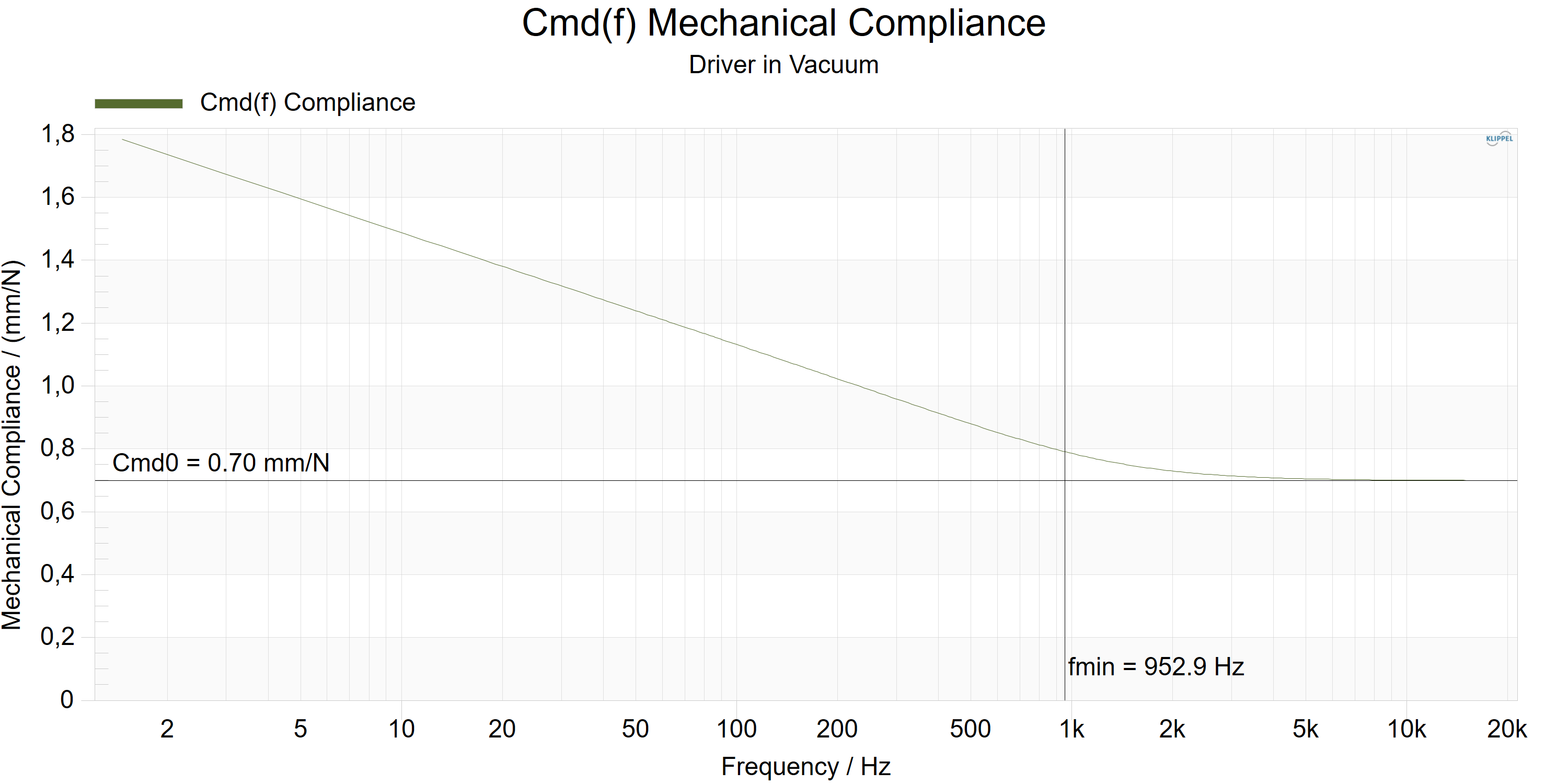
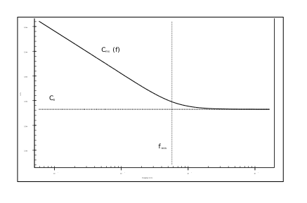
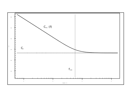
The result window shows the frequency dependent mechanical compliance. Since the Ritter creep model is selected, two additional parameters \(C_{\text{md0}}\) and \(f_{\text{min}}\) are overlayed, which display key figures of the model.
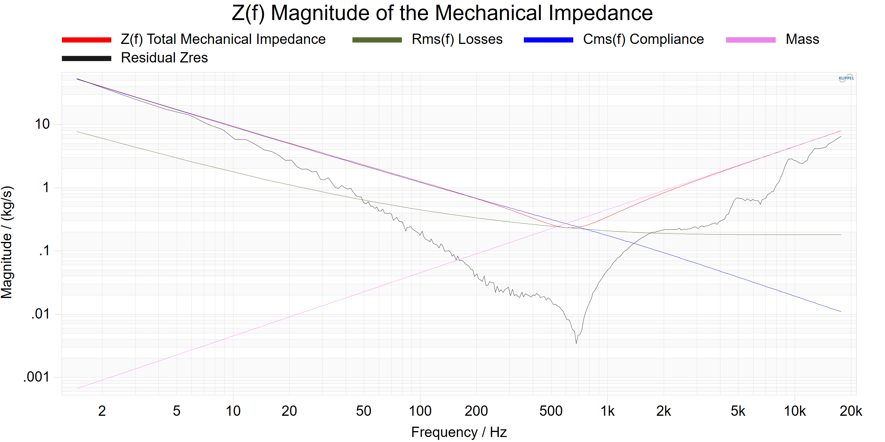
Z(f) Mechanical Impedance Magnitude#
The window shows the magnitude of the different mechanical impedances, related to the driver measurement in free air. The red curve shows the complete impedance, the black curve the residual part which cannot be explained by the model.
Performing a New MMT Measurement (Part 2)#
In the second part of the tutorial a step-by-step guide is provided to measure the electrical and mechanical driver parameters. We assume that the following standard hardware configuration is available:
Driver mounted in laser stand and / or Vacuum Measurement Kit
Setting up the Hardware#
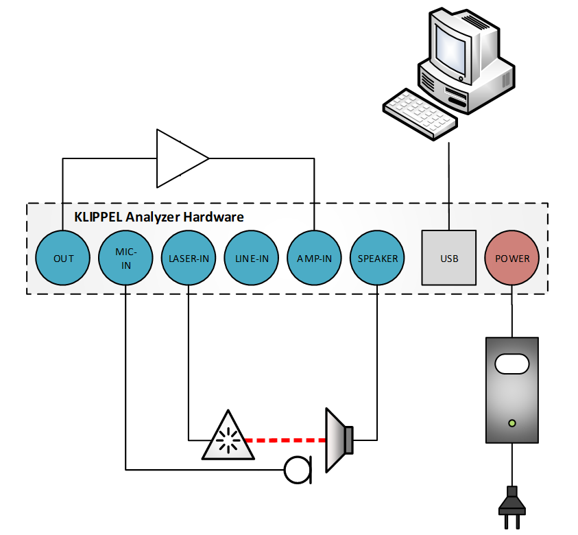
Connect the hardware components as described in the Hardware Manual. Depending on the method you use, you have to connect laser or microphone.
Note
For highly reflective or dark surfaces it may be required to make a dot with white ink (correction fluid) on the diaphragm and adjust the laser to this point. Alternatively, you can use white adhesive tape that can be removed easily after the measurement. See also section Laser Sensors in Hardware Manual for more information.
Perform the LPM Measurements#
Open the New Object dialogue and choose LPM Microspeaker Multipoint Tool
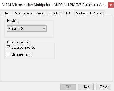
Select the operation 1a LPM T/S Parameter Air Center and open the property page Input. Make sure that the Laser signal is captured (Laser connected is checked) and select the speaker channel you are using for the measurement. It is also possible to connect a microphone to measure SPL in the near field, additionally, which will not be used by the MMT.
Open property page Stimulus shown below
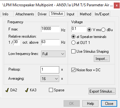
Specify \(f_{\text{max}}\) (upper frequency range of stimulus), relative resolution, reference frequency and voltage of the excitation signal. The specified voltage is either referred to the speaker terminals (at Speaker terminals) or to the amplifier input (at OUT 1). Select at Speaker terminals. In this case, the amplifier gain is measured prior to the parameter measurement and the excitation signal is adjusted to the measured gain. It is recommended to activate Noise floor monitoring.
Note
For more information on setting up the Linear Parameter Measurement (LPM), please refer to the LPM Manual
Open Property Page Method
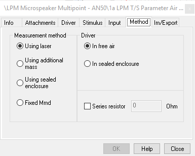
Select Using laser and In free air.
Place the laser according to the template name and start the measurement.
You may repeat steps 2 to 6 for the missing measurements (north, east, south, west, vacuum). If warnings or error occur, please refer to the LPM Manual.
Setting up the MMT Processing#
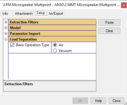
Select the operation 2 MMT Microspeaker Multipoint Tool and open the property page.
If no load measurement was performed, deactivate Basis Operation Type.
Start the Measurement#
Start measurement by clicking Run

After extracting the measurement data from the LPM operations, the processing will be performed. Depending on the available data and setup, you may get one of the warning messages discussed in the MMT - Reference.
View all result windows and tables by activating the checkboxes in the result window list. You may also define your own window arrangement and your own setting of default windows (Default windows are opened automatically if double clicked on the operation). For customizing result presentation, refer to the dBLab Manual.
Repeat the measurement, if necessary, by clicking Run
Customizing MMT (Part 3)#
In this part of the tutorial, we will discuss modifications of the setup parameters to use more powerful features and improve the performance of the measurement. Most of the topics discussed here are examined in greater detail in the same section of the LPM manual.
Physical Limitations#
Influence of Measurement Conditions#
The properties of the suspension depend on many factors (excitation level, time, ambient temperature, humidity). They usually vary by a significant amount depending on excitation level [1] , as well as temperature increase [2] in respect to the ambient temperature.
Adequate Modeling#
The measurement of the linear parameters fails if the model is not adequate for the particular driver. For example, additional electrical components, mechanical sub-resonance and acoustical guides may cause substantial deviations between the measured and expected behavior.
In contrary to the LPM module, the MMT offers advanced creep models to cope with particular high visco‑elastic effects of micro-speakers. By combining multiple measurements, the effect of rocking modes and other irregular vibrations can be compensated.
How to Get the Best Performance of the LPM Measurements?#
In this section a step-by-step procedure is outlined that maximizes the accuracy of the results. Factors that deteriorate the performance are identified and suggestions are made for improvements. For a detailed breakdown, please take a look at the LPM manual at the same section.
- Precise Calibration
Ensure that your measurement device and the needed sensors are calibrated. It is recommended to verify the calibration using a reference speaker. Note that e.g., a laser calibration error will deteriorate the accuracy of the mechanical parameters.
- Amplifier
Do not use DC-coupled amplifiers.
- Adjust Laser
Adjust the distance between the laser head and the diaphragm carefully. Make sure that the rest position of the diaphragm is in the middle of the laser’s working range. Move the diaphragm slightly with your fingers (if possible) and check that the working range is not left. To increase reflection, you may apply a white dot (white correction fluid or adhesive tape) on the diaphragm and adjust the laser to this point.
- Check Mounting of the Driver
Check that the driver is tightly mounted in the laser stand. Make sure that no cable, etc. touches the driver or the laser head.
- Use At Speaker Terminals
Select Voltage: at Speaker terminals in property page STIMULUS of the LPM.
- Use Speaker Channel 2 (Distortion Analyzer only)
Depending on the device you are using, there are some special configurations of channel 2 (e.g., higher current sensing sensitivity).
Note
Note that the KA3 supports switching current sensitivity per channel (Hardware manual for details).
- Adjust Frequency Range
Adjust the frequency range in property page Stimulus if this is required by the application or type of DUT. Choose the spectral resolution (lines per octave) depending on the fitting accuracy of \(f_{\text{s}}\). Higher values (dense spectrum) will cause the activation of more distortion, but improves \(f_{\text{s}}\) fitting accuracy, and vice versa.
- Adjust Excitation Level
The excitation voltage needs to be adjusted carefully. Select Noise floor monitoring in property page Stimulus. This will invoke an additional (zero stimulus) noise floor measurement before the main measurement.
- Check Laser Spectrum
Check that the SNR+D ratio is at least 20 dB. If you are measure with Noise floor monitoring, the distortion in the displacement spectrum should be sufficiently low.
- Reducing Noise Level
All the sensors used for measuring sound pressure, displacement, voltage and current add noise to the measured signal. You may reduce any noise component, which is uncorrelated to the stimulus by activating the averaging in the property page Stimulus. We recommend to average over at least 16 measurements.
- Increasing Signal to Noise Ratio for High Q Drivers
Due to the dip in the current spectrum the signal to noise ratio sometimes decreases rapidly at the resonance frequency. The SNR+D is limited by distortion as usually highest distortion is created around the resonance. This dip can be flattened considerably if a stimulus shaping is applied.
For more information on this problem, please refer to the LPM manual.
How to Use Different Inductance Models#
The inductance and the magnetic losses of most drivers are strongly frequency dependent and show a very complex behavior. The MMT supports various models to fit this behavior. They can be selected in the category Model.
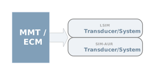
See section MMT-Reference Linear Modeling Inductance Model for detailed information. Always use the LR2 model (Shunted Inductor model) if you want to export the results to the SIM – Simulation and SIM-AUR – Nonlinear Simulation and Auralization module.
How to Use Different Creep Models#
The suspension creep at low frequencies is strongly frequency dependent and shows a very complex behavior. The MMT supports various models to fit this behavior. They can be selected in the category Model.
See section MMT-Reference Linear Modeling Creep Model for detailed information. Always use the Log model if you want to export the results to the SIM – Simulation and SIM-AUR – Nonlinear Simulation and Auralization module.
Importing Mms, Bl, Re#
The fitting algorithm fits all parameters automatically to the measured impedance data by default. However, it might be desirable to define fixed values since they are measured or known by other methods. In the Imported values category fixed values for \(M_{\text{ms}}\) , \(Bl\) and \(R_{\text{e}}\) can be specified. If the user sets or modifies these values the fitting algorithm tries to fit all other parameters except the fixed ones. Please note that all parameters are refitted if one of the fixed parameters are changed.
How to Measure Drivers with Different Loads?#
The MMT supports measurements performed in air, vacuum and with an attached enclosure. It automatically detects the type of the measurement by certain keywords in the LPM measurement name:
- air
Measurement performed in air
- vac
Measurement performed in vacuum
- load
Measurement performed with attached load (e.g., in enclosure)
If more than one measurement of one type is detected, spatial averaging is performed automatically performed.
It is recommended to perform measurements with complex loads in the following order:
Perform measurements in air at different positions. This will cope with potential rocking modes or other parasitic vibrations.
Measure the speaker in vacuum. This measurement is used to determine the pure mechanical parameters. If necessary, perform more than one measurement to cope with parasitic vibrations.
Measure the speaker attached in the enclosure. If it’s more applicable, you may also start with this step.
Activate the Load Separation in the MMT. The base operation type with air is mostly the most interesting separation result, so it is set by default. Change the parameter if you find it necessary. For more information on the load separation, see section MMT-Reference Linear Modeling Load Separation.
MMT - Reference#
Overview#
The MMT Multipoint Measurement Tool offers acquisition of precise Thiele/Small parameters by evaluating a set of LPM – Linear Parameter Measurement taken from one transducer. Using a set of LPM measurements offers the opportunity to reduce the variation of the linear parameters due to rocking modes or other vibrational defects. To cope for the significant visco‑elastic behavior, typically found in micro-speakers, advanced creep models are used. By using measurements taken in vacuum, air and/or with an attached load (e.g., an enclosure) the impact of air to the transducer can be calculated, displayed and evaluated. Displacement measurements taken on different points of the membrane are averaged to improve the accuracy of the measured force factor \(Bl\), and derived parameters.
Linear Modeling#
Creep Modeling#
The traditional Thiele/Small Loudspeaker Model considers the compliance of the suspension (\(C_{\text{ms}}\)) and the mechanical losses (\(R_{\text{ms}}\)) constant parameters. Taking the creep effect of the suspension into account, these parameters become frequency dependent.
The KLIPPEL LPM module (dB-Lab \(\leq\) 212) offers a creep model with a frequency dependent compliance increasing towards lower frequencies, but still constant losses:
This simple model delivers good results for speakers with low creep effect, but yields fitting results of limited accuracy for speakers with a high creep effect.
Both new models consider the compliance \(C(f)\) to be complex. Thus, interpreting the compliance as a spring is not appropriate anymore.
Splitting the complex impedance of the compliance \(Z_{C}\) into its real and imaginary part makes it possible to consider it to be a series connection of a spring and a dashpot:
with
The dashpot modeling the frequency dependent losses of the suspension \(R_{C_{\text{ms}}}\left( f \right)\) can be added to the constant losses \(R_{\text{ms0}}\), which results into the total mechanical losses \(R_{\text{ms}}(f)\). Thus, the equivalent circuit of the transducer will remain the same, just considering the losses and the compliance to be frequency dependent.
Knudsen Creep Model#
Knudsen proposed a model for the suspension creep [3] using a logarithm weighted with the creep factor \(\lambda\):
This model is purely mathematical, based on the experience that the creep increases nearly linear towards lower frequencies, when viewed on a semi-logarithmic scale.
The parameter \(C_{0}\) contains the value of the real part at the resonance frequency \(f_{\text{s}}\) but is not equal to the value of the compliance \(C_{\text{ms}}(f_{\text{s}})\) when using the notation of formula (2).
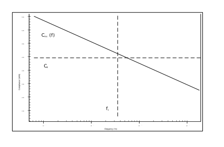
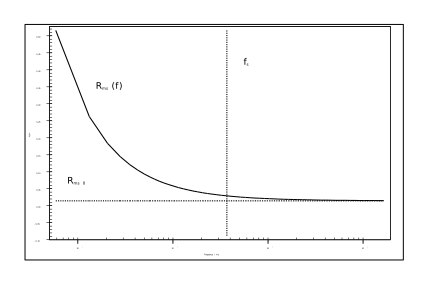
The model integrated in the LPM module is based upon this model, but neglects the complex argument of the logarithm and thus the frequency dependence of the mechanical losses.
Ritter Creep Model#
A three-parameter model based on retardation spectra was introduced by Ritter [4] .
Instead of becoming negative towards high frequencies the creep reaches a minimum compliance, which is described by \(C_{0}\).
The frequency \(f_{\text{min}}\) corresponds to the minimum retardation time of the retardation spectra and can be interpreted as the frequency where the creep of the suspension starts to rise.
This model is rather complex, but delivers best fitting results, with just one additional parameter.
Load Separation#
Air Measurement#
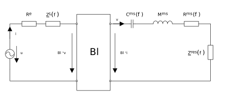
The circuit shown in Figure 5 models the transducer measured in air. The mechanical parameters \(R_{\text{ms}}\) , \(C_{\text{ms}}\) and \(M_{\text{ms}}\) represent mechanical as well as acoustical qualities.
The additional impedance \(\underline{Z}_{\text{res}}\) (residual impedance) represents all effects which are not covered by the three mechanical parameters. This will mainly incorporate frequency dependent effects like air leakage, since the frequency dependence of the compliance and the losses are considered to be purely mechanical due to the creep of the suspension.
Vacuum Measurement#
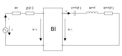
Measuring a speaker in vacuum neglects all influences of air; thus, an estimation of the purely mechanical and electrical parameters becomes possible.
Figure 6 shows the electrical equivalent circuit used for vacuum measurements. The classical mechanical parameters \(R_{\text{ms}}\) , \(C_{\text{ms}}\) and \(M_{\text{ms}}\) describe the behavior of the transducer in air and are replaced by the purely mechanical parameters \(R_{\text{md}}\) , \(C_{\text{md}}\) and \(M_{\text{md}}\). Since measurement in vacuum is considered free of air and acoustical load, the additional impedance is necessary.
Load Measurement#
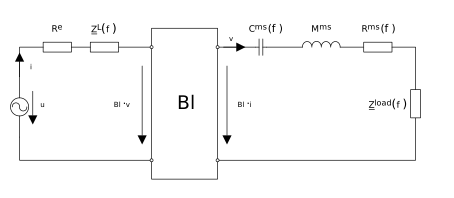
Attaching a load to a transducer can have different meanings. In any case it will add a mechanical (e.g., adding a panel to a shaker) or an acoustical system (e.g., adding a horn to a compression driver) or a mixture of both to the transducer.
Figure 7 shows the circuit used to model the load measurement. The load impedance \(Z_{\text{load}}\) incorperates all qualities which are not covered by the electrical parameters or the mechanical parameters measured in air. (Note: You may also calculate the load from the difference of the speaker measured in vacuum and with load)
Thus \(Z_{\text{load}}\) represents a system of arbitrary order depending on the attached load.
Spatial Averaging#
Especially the estimation of the force factor \(Bl\) with a laser measurement is very prone to resonant modes of the transducer, since the estimation is directly proportional to the displacement of the membrane.
To get more reliable results it is recommended to measure the displacement with a laser at different points on the membrane. The MMT Multipoint Measurement Tool will automatically average these measurements for a more robust estimation.
Estimation Order#
The following listings display the desired order to estimate the linear transducer parameters.
If possible, \(Bl\) is identified using the air measurement. If \(Bl\) cannot be identified, the measured Bl from the load measurement is taken (or from the vacuum measurement if the load measurement does not provide a valid \(Bl\))
Vacuum Measurement#
DC resistance \(R_{\text{e}}\) (alternative from air measurement)
Inductivity model \(Z_{L}\) (alternative from air measurement)
Creep model (alternative from air measurement)
Mechanical parameters (\(R_{\text{md}}\) , \(C_{\text{md}}\) and \(M_{\text{md}}\))
Free Air Measurement#
Mechanical parameters in air (\(Bl\) , \(R_{\text{ms}}\) , \(C_{\text{ms}}\) and \(M_{\text{ms}}\))
Residual impedance \(Z_{\text{res}}\)
Load Measurement#
Load impedance \(Z_{\text{load}}\)
Property Pages#
Select the MMT operation in the project window, and click the View properties button  .
.
Input Category#
The category Input specifies the input data of the Multipoint Measurement Tool.
- Extract Laser Signals \(H_{x}(f)\)
If activated, the \(H_{x}(f)\) curve, representing the transfer function between displacement signal \(X(f)\) and stimulus \(U(f)\), of every matching LPM operation is extracted and used for the fitting.
- Operation Filter
- Range: Include, Exclude
If activated, specify if LPM operations containing a specific string shall be used or ignored as input data.
- Include/Exclude Containing
- Range: Include, Exclude
LPM operations with this part will be included / excluded.
Model Category#
The category Model specifies models used to for frequency dependent elements of the Multipoint Measurement Tool.
- Inductance Model
- Range: none, LR2, Leach, Wright
Inductance model used for the fitting of the high frequency part of the impedance \(Z_{\text{e}}(f)\). Different models will yield different accuracy for specific drivers.
- Creep Model
- Range: none, Log, Knudsen, Ritter
Model used to fit the creep effect of the transducer compliance \(C(f)\) at low frequencies.
Imported Values Category#
The category Imported Values allows to enter known values for the Multipoint Measurement Tool, which can be used to improve the fitting process.
- \(Bl\)
- \(Bl\) in N/ARange: \(>\) 0
Force factor
- \(M_{\text{ms}}\)
- \(M_{\text{ms}}\) in gRange: \(>\) 0
Mechanical moving mass (in free air)
- \(R_{\text{e}}\)
- \(R_{\text{e}}\) in \(\Omega\)Range: \(>\) 0
Electrical DC-resistance
Load Separation Category#
The category Load Separation holds properties which are related to separating loads in drivers, if a matching LPM operation present.
- Basis Operation Typ
- Range: Air, Vacuum
Defines the basis operation for load separation. This means, the load will be separated from the measurement type specified here (if present). If deactivated, no load separation is performed.
Display Category#
The category Display holds properties which modify the presentation of the measurement results.
- Align Measurement Curves
If active, measured curves are aligned near the fitted curves. This option is intended to aid the interpretation of the fitting quality.
Result Windows#
Table Linear Parameters#
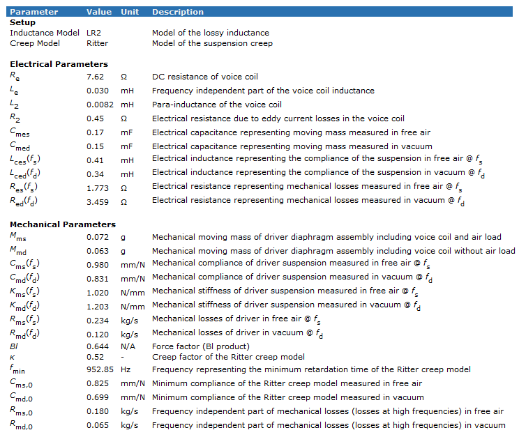
The result window shows the electrical and mechanical parameters of the linear driver model, the derived parameters (resonance frequency, loss factors etc.) and the parameters of the suspension creep model that are determined by the MMT. Also, this window will show fitting related warnings and errors.
Electrical Parameters#
- \(R_{\text{e}}\)
- \(R_{\text{e}}\) in \(\Omega\)
DC resistance of driver voice coil
- \(L_{\text{e}}\)
- \(L_{\text{e}}\) in mH
Lumped elements of para-inductance
- \(L_{2}\)
- \(L_{2}\) in mH
Lumped elements of para-inductance
- \(R_{2}\)
- \(R_{2}\) in \(\Omega\)
Lumped elements of para-inductance
- \(K\)
Parameters of the Leach inductance model
- \(N\)
Parameters of the Leach inductance model
- \(K_{\text{rm}}\)
Parameters of the Wright inductance model
- \(E_{\text{rm}}\)
Parameters of the Wright inductance model
- \(K_{\text{xm}}\)
Parameters of the Wright inductance model
- \(E_{\text{xm}}\)
Parameters of the Wright inductance model
- \(R_{\text{es}}\)
- \(R_{\text{es}}\) in \(\Omega\)
Electrical resistance due to mechanical losses in free air
- \(R_{\text{ed}}\)
- \(R_{\text{ed}}\) in \(\Omega\)
Electrical resistance due to mechanical losses in vacuum
- \(C_{\text{mes}}\)
- \(C_{\text{mes}}\) in µF
Electrical capacitance representing moving mass in free air
- \(C_{\text{med}}\)
- \(C_{\text{med}}\) in µF
Electrical capacitance representing moving mass in vacuum
- \(L_{\text{ces}}\)
- \(L_{\text{ces}}\) in mH
Electric inductance representing driver compliance in free air
- \(L_{\text{ced}}\)
- \(L_{\text{ced}}\) in mH
Electric inductance representing driver compliance in vacuum
- \(f_{\text{s}}\)
- \(f_{\text{s}}\) in Hz
Driver resonance frequency in free air
- \(f_{\text{d}}\)
- \(f_{\text{d}}\) in Hz
Driver resonance frequency in vacuum
Loss Factors#
- \(Q_{\text{tps}}\)
Total quality-factor considering all losses in free air
- \(Q_{\text{tpd}}\)
Total quality-factor considering all losses in vacuum
- \(Q_{\text{ms}}\)
Mechanical quality-factor measured in free air considering \(R_{\text{ms}}\) only
- \(Q_{\text{md}}\)
Mechanical quality-factor measured in vacuum considering \(R_{\text{md}}\) only
- \(Q_{\text{es}}\)
Electrical quality-factor measured in free air considering \(R_{\text{e}}\) only
- \(Q_{\text{ed}}\)
Electrical quality-factor measured in vacuum considering \(Re\) only
- \(Q_{\text{ts}}\)
Total quality-factor measured in free air considering \(R_{\text{ms}}\) and \(R_{\text{e}}\)
- \(Q_{\text{td}}\)
Total quality-factor measured in vacuum considering \(R_{\text{md}}\) and \(R_{\text{e}}\) only
Mechanical Parameters#
- \(M_{\text{ms}}\)
- \(M_{\text{ms}}\) in g
Mechanical moving mass of driver diaphragm assembly including voice coil and air load
- \(M_{\text{md}}\)
- \(M_{\text{md}}\) in g
Mechanical moving mass of driver diaphragm assembly including voice coil without air load
- \(C_{\text{ms}}\)
- \(C_{\text{ms}}\) in mm/N
Mechanical compliance of driver suspension measured in free air
- \(C_{\text{md}}\)
- \(C_{\text{md}}\) in mm/N
Mechanical compliance of driver suspension measured in vacuum
- \(K_{\text{ms}}\)
- \(K_{\text{ms}}\) in N/mm
Mechanical stiffness of driver suspension measured in free air
- \(K_{\text{md}}\)
- \(K_{\text{md}}\) in N/mm
Mechanical stiffness of driver suspension measured in vacuum
- \(R_{\text{ms}}\)
- \(R_{\text{ms}}\) in kg/s
Mechanical losses of driver in free air
- \(R_{\text{md}}\)
- \(R_{\text{md}}\) in kg/s
Mechanical losses of driver in vacuum
- \(Bl\)
- \(Bl\) in N/A
Force factor (\(Bl\)-product)
Creep Parameters#
- \(\lambda\)
Suspension creep factor
- \(\kappa\)
Creep factor of the Ritter creep model
- \(f_{\text{min}}\)
- \(Bl\) in Hz
Frequency representing the minimum retardation time of the Ritter creep model
Fitting Parameters#
- \(\text{rmse}\: Z_{\text{air}}\)
- \(\text{RMSE}_{Z,\text{air}}\) in %
root-mean-square fitting error of the driver impedance \(Z(f)\) measured in air
- \(\text{rmse}\: Z_{\text{vac}}\)
- \(\text{RMSE}_{Z,\text{vac}}\) in %
root-mean-square fitting error of the driver impedance \(Z(f)\) measured in vacuum
- \(\text{rmse}\: H_{x,\text{air}}\)
- \(\text{RMSE}_{Hx,\text{air}}\) in %
root-mean-square fitting error of the driver transfer function \(H_{x}(f)\) measured in air
- \(\text{rmse}\: H_{x.\text{vac}}\)
- \(\text{RMSE}_{Hx.\text{vac}}\) in %
root-mean-square fitting error of the driver transfer function \(H_{x}(f)\) measured in vacuum
LPM Data Information#
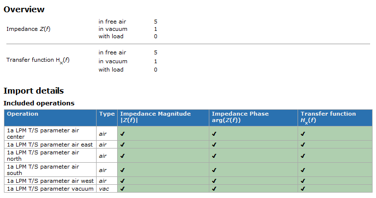
The result window shows detailed information about the extracted (and ignored) data. At top, you will find a small summary about the extracted data. Underneath, all found LPM operations are listed, showing the extracted data. The column Type helps to understand the assignment of the operation to a measurement type. Different colors mark different extraction states: a green background marks extracted, a red background missing data (if e.g., one LPM operation was measured without laser). LPM operations without data are marked grey. Ignored LPM operations are listed last.
Z(f) Impedance Magnitude, Z(f) Impedance Phase#
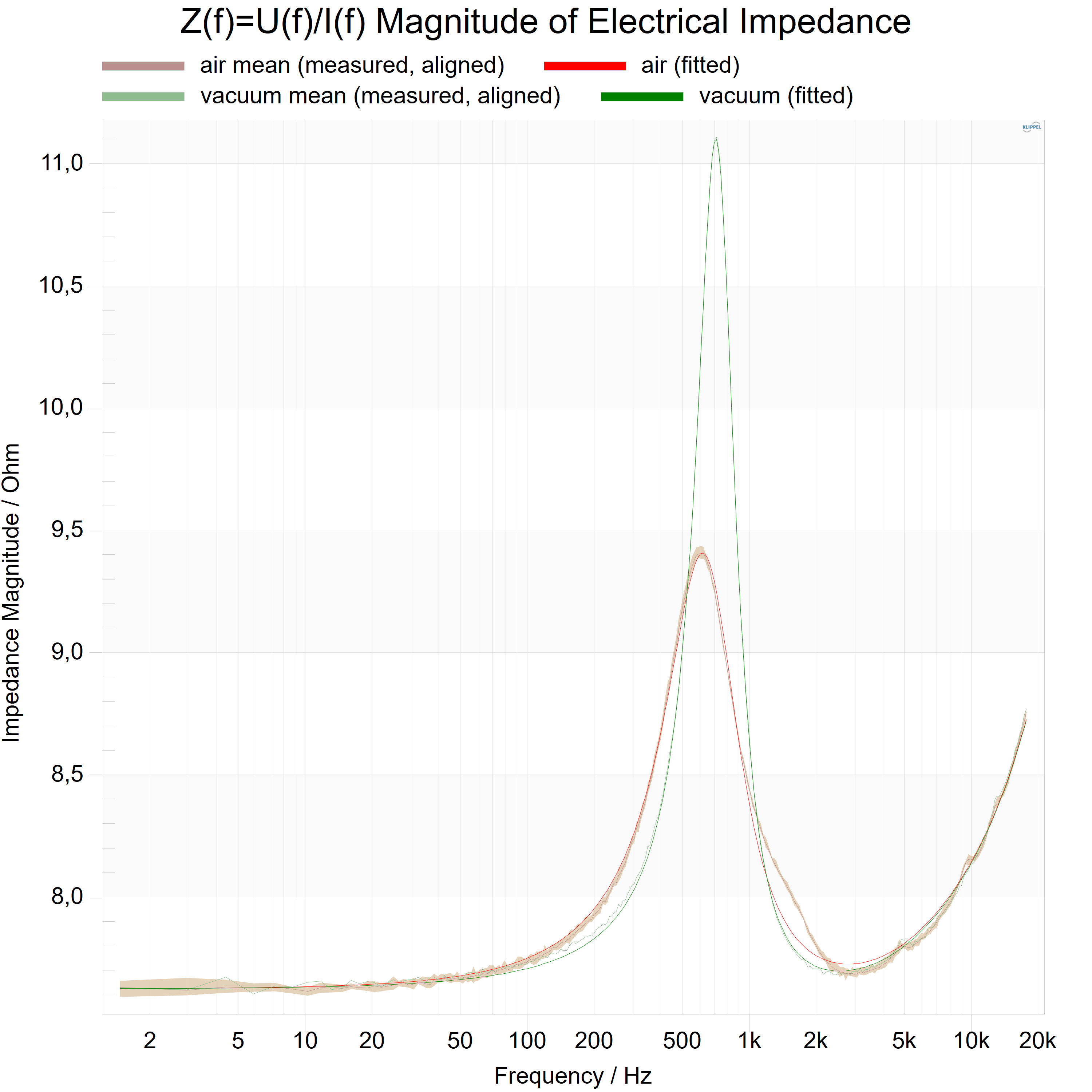
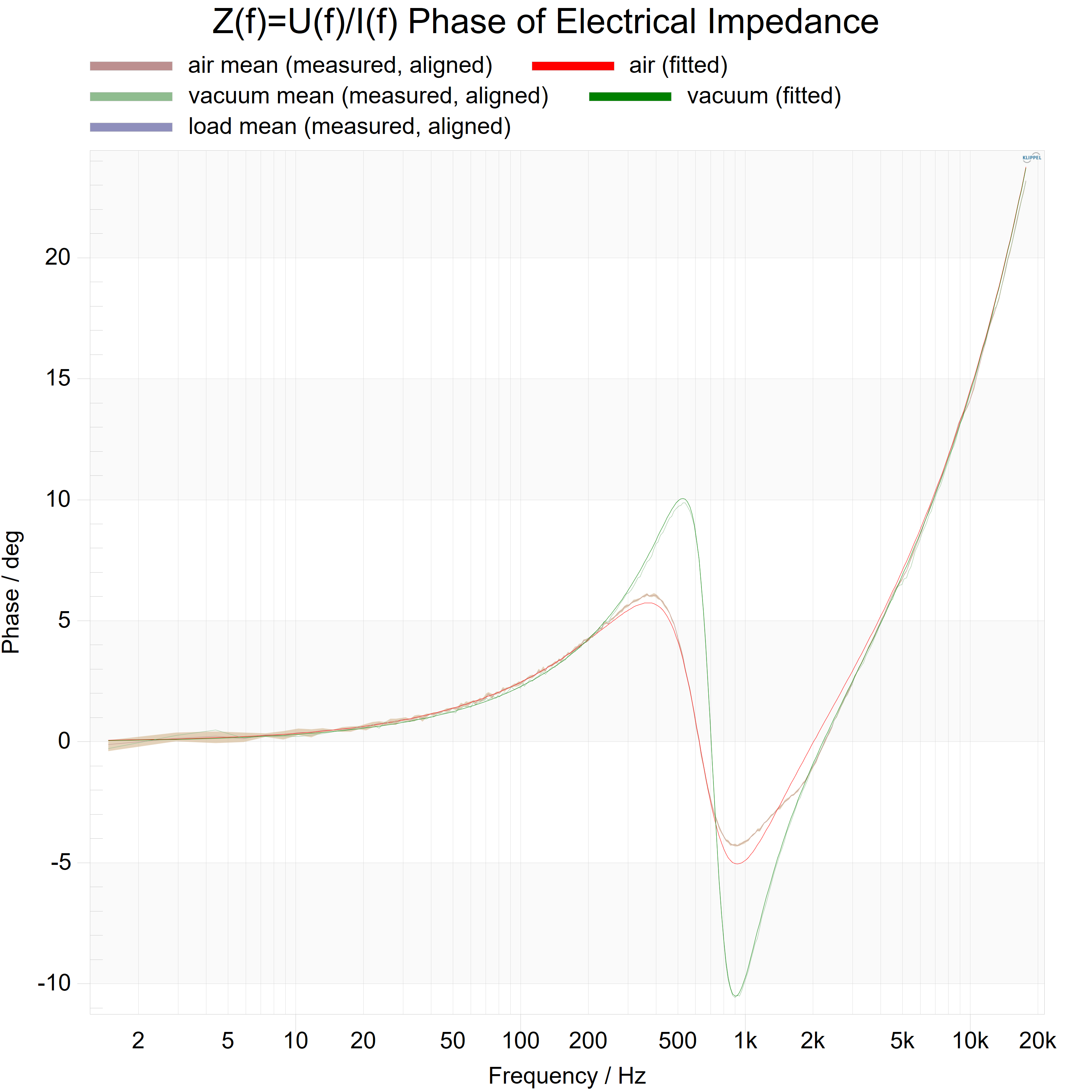
The two result windows show the magnitude and the phase response of the measured and estimated impedance \(Z(f) = \frac{U(f)}{I(f)}\) , where \(U(f)\) is the terminal voltage and \(I(f)\) is the current. Measured curves are the ratio of the measured spectra \(U(f)\), while \(I(f)\) ; fitted curves represent the impedance of the linear driver equivalent circuit using the linear model and the identified electrical parameters.
If more than one measurement of a type is detected, the mean value of all curves is drawn, as well as an area marking the minimum and maximum values.
H(f) Magnitude#
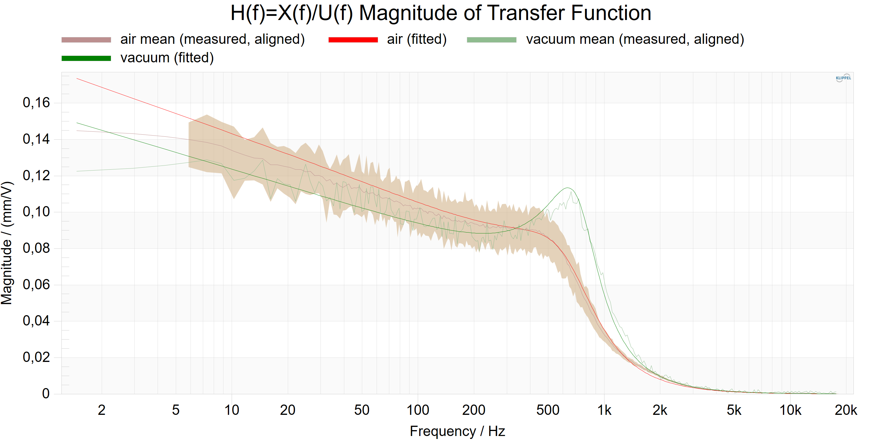
The result window shows the magnitude of the measured and estimated transfer function \(H_{x}(f) = \frac{X(f)}{U(f)}\) between the voice coil displacement \(X(f)\) and the terminal voltage \(U(f)\). Measured curves are the ratio of the measured spectra \(X(f)\), \(U(f)\); fitted curves represent the transfer function based on the linear driver equivalent circuit using the identified electrical and mechanical parameters as well as the creep parameter.
Note
This window is only available if \(H_{x}(f)\) extraction was selected in the INPUT category of the property page.
Z(f) Mechanical Impedance Magnitude#
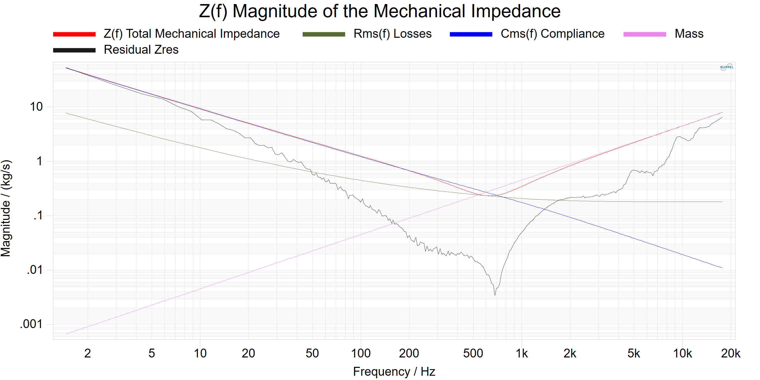
The result window shows the magnitudes of different mechanical impedances related to the driver measured in free air. If there is no air measurement but a vacuum measurement available, this will be displayed. The figure demonstrates how the mass dominates the total mechanical impedance towards higher and the compliance towards lower frequencies respectively. At the resonance frequency the total impedance becomes real and reaches the value of the losses. The residual impedance indicates how much of the transducer behavior in free air is not covered by the rest of the model.
Note
The residual impedance includes effects which aren’t modeled (e.g., air leakage), as well as fitting errors.
Z(f) Mechanical Magnitude, Z(f) Mechanical Phase (load separation)#
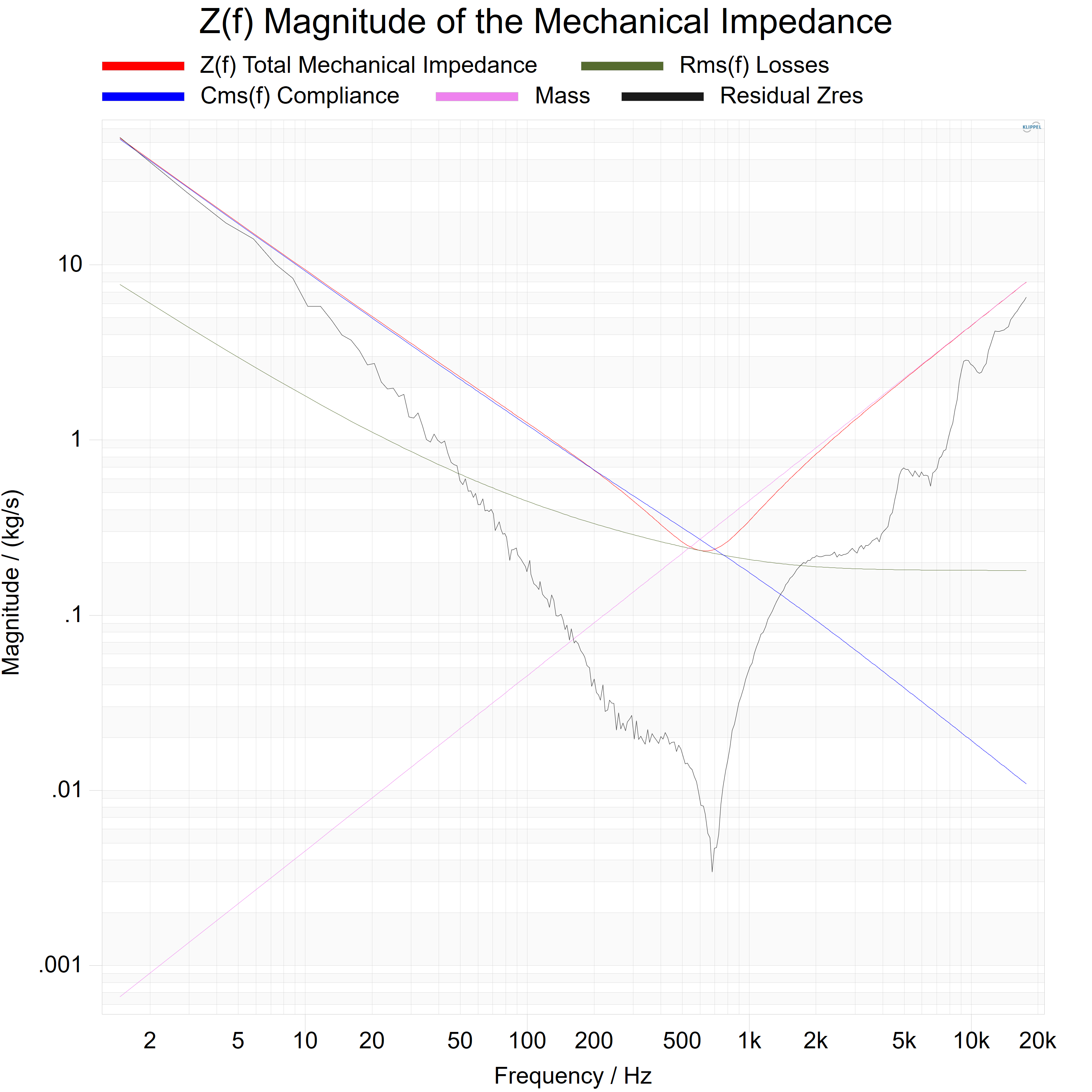
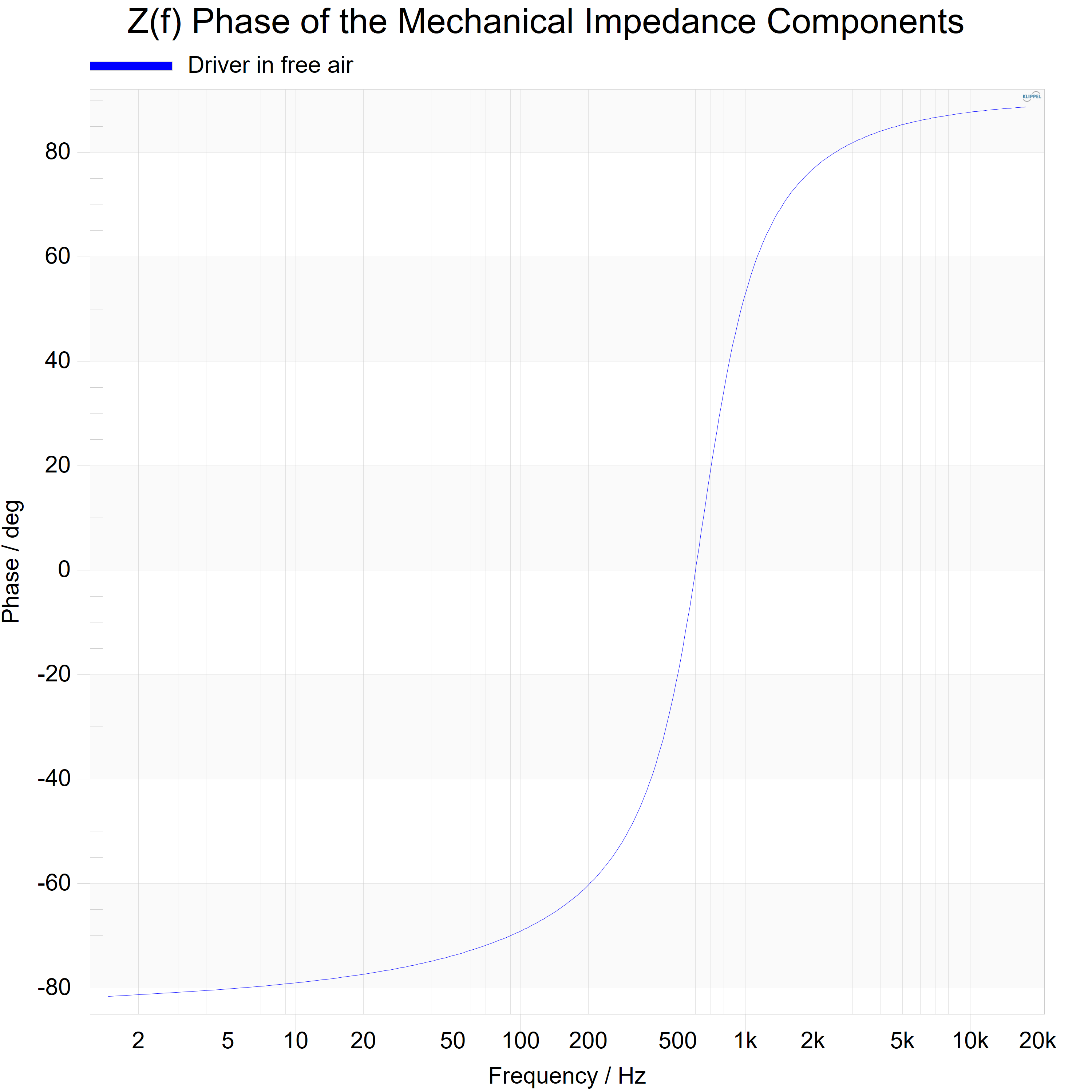
The result window shows the magnitude and phase of the mechanical impedance \(Z(f) = \frac{F(f)}{v(f)}\). These curves give an outline of the qualities of the connect load and how it influences the behavior of the transducer.
Under the Assumption that the corresponding curves are available, you may select the domain using Basis Operation Type in the property page category Load Separation.
- Air
calculates the load using the air measurement(s) as basis
- Vacuum
calculates the load using the vacuum measurement(s) as basis
Cms(f), Cmd(f) Mechanical Compliance#
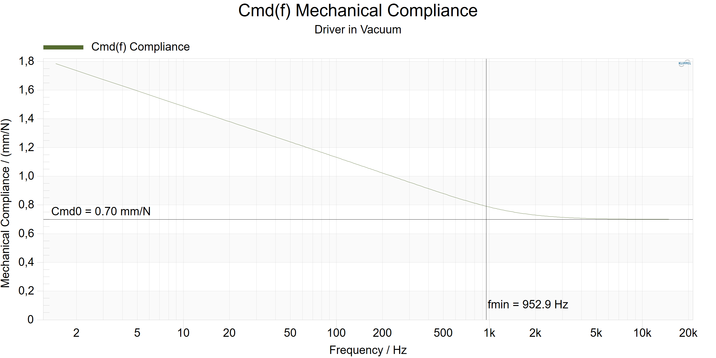
The result window shows the frequency dependence of the mechanical compliance \(C(f)\). Depending on the available data, it will be taken from either the air, or the vacuum measurement. Note that the vacuum measurement will be preferred, since it represents the pure mechanical parameters (see Vacuum Measurement).
If the Ritter creep model is selected, the two parameters \(C_{\text{md0}}\) (resp. \(C_{\text{ms0}}\) if no vacuum measurement is available) and \(f_{\text{min}}\) are displayed as well. See Table Linear Parameters for the parameter description.
Supported Modules for Im/Export#
Malfunctions and Troubleshooting#
Overview#
This chapter will provide information that can help you solve common problems that occur with the Klippel Analyzer and the MMT module. The software generates a variety of warnings automatically if the signals are badly conditioned or a malfunction is detected. Some warnings may be neglected but it is always recommended to find out the cause of the problem.
If you cannot find a description here that matches your problem, try these options:
Error and Warning Messages#
No Measurement Data Available#
- Cause:
No LPM operation could be found, or no LPM operation holds valid data, in the Driver object.
- Remedy:
Make sure that at least one LPM measurement is available in your Driver object. Check your LPM operations and solve errors which may cause problems with the measurement. See LPM manual for more details.
No Mechanical Calibration#
- Cause:
No \(H_{x}(f)\) data was extracted from the LPM, or no \(Bl\) or \(M_{\text{ms}}\) were specified.
- Remedy:
Activate the option to extract the \(H_{x}(f)\) curves from the LPM operation, or specify \(Bl\) or \(M_{\text{ms}}\).
Could Not Fit Selected Inductance Model#
- Cause:
The selected inductance model is not sufficient for your measured driver.
- Remedy:
Select another inductance model in the category Model.
Could Not Fit Selected Creep Model#
- Cause:
The selected creep model is not sufficient for your measured driver.
- Remedy:
Select another creep model in the category Model.
Could Not Fit Mechanical Impedance with Imported Re#
- Cause:
Mismatch between imported \(R_{\text{e}}\) and fitted \(R_{\text{e}}\)
- Remedy:
Check if the right \(R_{\text{e}}\) value was imported.
Load Separation Disabled#
- Cause:
Load separation could not be performed for the found measurements (e.g. an LPM measurement with the driver in the enclosure was not performed).
- Remedy:
Perform an LPM operation of the driver in the target load.
Literature#
Papers#
[1] M.H. Knudsen and J.G. Jensen, “Low-Frequency Loudspeaker Models that Include Suspension Creep,” J. Audio Eng. Soc., vol. 41, pp. 3-18, (Jan./Feb. 1993)
[2] F. Agerkvist and T. Ritter, “Modelling Viscoelasticity of Loudspeaker Suspensions using Retardation Spectra,” presented at the 129th Convention of the Audio Engineering Society, San Francisco, November 4-7, 2010, preprint 8217
[3] W. Klippel and U. Seidel, “Fast and Accurate Measurement of Linear Transducer Parameters,” presented at the 110th Convention of the Audio Engineering Society, Amsterdam, May 12-15, 2001, preprint 5308
[4] K. Thorborg, A. Unruh and C. Struck, “An Improved Electrical Equivalent Circuit Model for Dynamic Moving Coil Transducers”, presented at the 122nd Convention of the Audio Engineering Society, Vienna – Austria, May 5-8, 2007
[5] K. Thorborg, C. Tinggaard, F. Agerkvist and C. Futtrup, “Frequency Dependence of Damping and Compliance in Loudspeaker Suspensions”, J. Audio Eng. Soc. Vol. 58 no. 6, June 2010.
[6] K. Thorborg and C. Futtrup, “Electro-Dynamic Transducer Model Incorporating Semi-Inductance and Means for Shorting AC-Magnetization”, J. Audio Engineering Society, vol.59 September 2011.
