MSPM – Micro Suspension Part Measurement

MSPM – Micro Suspension Part Measurement#

MSPM - Tutorial#

Overview#

MSPM Lite and MSPM Pro#

KLIPPEL MSPM includes two modules for the measurement of small diaphragms. The MSPM Lite is dedicated to the measurement of the linear parameters like mechanical stiffness K and resonance frequency in the small signal domain.

The MSPM Pro is additionally capable of measuring the nonlinear stiffness \(K(x)\) of small membranes for high displacements.

The suspension part measurement is a dynamic, nondestructive technique which excites the membranes pneumatically under similar conditions as operated in the final application (e.g. micro speaker).

The Measurement Method#

MSPM Lite#

The MSPM Lite focuses on the accurate measurement of linear parameters in the small signal domain. The membrane is excited pneumatically by sound pressure in an enclosure and both pressure and displacement of the DUT (Device Under Test) are measured. Analyzing the transfer function between displacement and sound pressure provides the resonance frequency and \(Q\)-factor of the DUT. By measuring the moving mass using the Added Mass Method or using a high precision scale, the complete set of linear parameters can be calculated.

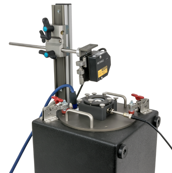
The LST Bench may be used as stand for the small measurement enclosure and provides the external rack for mounting the laser displacement sensor. The picture below shows the full measurement setup. The MSPM Bench is equipped with a small woofer producing suitable sound pressures for the measurement method. An additional inlay for the enclosure can reduce the air volume to increase the pressure.

The microphone as well as the laser sensor are powered by the measurement hardware. This platform also generates the stimulus provided via a power amplifier to the loudspeaker. The TRF – Transfer Function Measurement generates the sinusoidal sweep and measures displacement and sound pressure and calculates the transfer function out of it. The MSPM Lite extracts the important curves from the TRF Modules and calculates the linear parameters.

MSPM Pro#

The nonlinear stiffness \(K(x)\) of the micro speaker membranes is measured versus displacement \(x\) over the full range of operation. The nonlinear parameters are estimated from the measured displacement signal of the DUT plus the expected stimulating force on the DUT inside the pressure chamber. Since the sound pressure inside the enclosure is very high, a transfer function from the driving speaker’s input current to the driving force is used as a good approximation for the large signal domain.

The MSPM Pro uses the same measurement setup as the MSPM Lite.

The multi-tone stimulus for this measurement is generated by the LPM – Linear Parameter Measurement and the displacement of the DUT, current, voltage and sound pressure are measured. The MSPM Pro extracts the important curves from the LPM Modules and calculates the nonlinear stiffness.

For this measurement also a set of linear parameters is needed (linear mechanical stiffness \(K\), mechanical losses \(R\), moving mass \(m\)). Therefore, it is recommended to use the MSPM Lite and the MSPM Pro in combination.

MSPM Setup#

Overview#

Step-by-step instructions are provided to setup the hardware of the MSPM for the first time. It is assumed that the measurement bench is in the original packaging provided by the manufacturer. Please find additional instructions for installing the dB-Lab – Software and general information related to the KLIPPEL Analyzer Hardware in the dedicated manuals.

The setup uses the following components:

LST bench as stand for the measurement setup (or alternatives)
MSPM bench
Klippel Analyzer 3 (KA3) or Distortion Analyzer (DA2) hardware
Amplifier + XLR cable
Amplifier cable with speakON connector
Speaker cable
Laser displacement sensor (LK-H052)
Microphone (high pressure)
TRF – Transfer Function Measurement for the MSPM Lite
LPM – Linear Parameter Measurement for the MSPM Pro
MSPM Lite module
MSPM Pro module

Work Bench#

List of Parts#

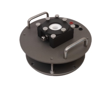
1 MSPM bench: Units: 1

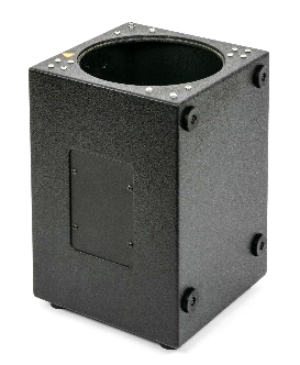
2 LST box: Units: 1

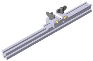
3 Laser rack: Units: 1

4 Mounting screws for laser rack: Units: 2
5 Discs for screws (5): Units: 2
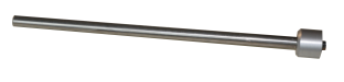
6 Laser rod: Units: 1

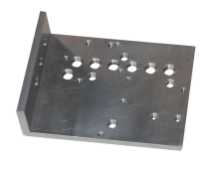
7 Laser platform: Units: 1

8 Laser Bracket: Units: 1
9 Disc for laser: Units: 2

Dimensions: M4
10 Allen screw for laser head: Units: 2

Dimensions: M4 x 25
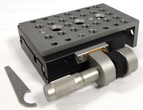
11 Translation Stage: Units: 1

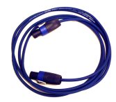
12 Cable speakON: Units: 1

Dimensions: 4 x 2.5 mm², 5 m

13 Tool for Allen screw (for laser): Units: 1

Dimensions: 2 mm
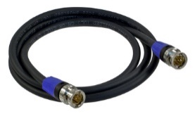
14 BNC cable: Units: 1

Dimensions: 5 m

15 Tool for Allen screw (for laser rack): Units: 1

Dimensions: 5 mm
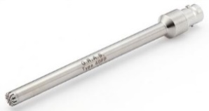
16 High pressure microphone: Units: 1

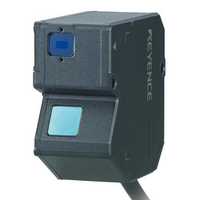
17 Laser displacement sensor set incl. cables: Units: 1

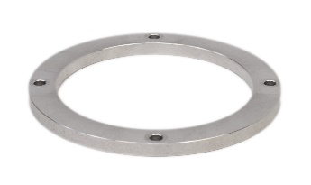
18 Extended Clamping Ring: Units: 1

Dimensions: 70 mm

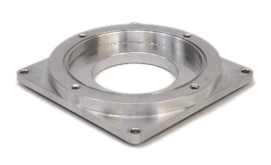
19 Extended Clamping Adapter: Units: 1

20 Sealing ring set included with MSPM bench rev. >= 1.1

72 x 1 mm (2 units): between extended lower clamping and DUT carrier

1 x spare
53 x 1 mm (3 units): between support and enclosure (pre-mounted)

between enclosure and standard lower clamping (pre-mounted)

between enclosure and extended lower clamping (pre-mounted)
47 x 1 mm (2 units): between standard lower clamping and DUT carrier

1 x spare
42 x 1 mm (1 unit): between enclosure and Volume Reducer (pre-mounted)

21 Sealing ring set included with MSPM bench rev. = 1.0

53 x 1 mm (2 units): between Support and enclosure (pre-mounted)

between enclosure and standard lower clamping (pre-mounted)
47 x 1 mm (2 units): between standard lower clamping and DUT carrier

1x spare
42 x 1 mm (1 unit): between enclosure and volume reducer (pre-mounted)

Mounting Instructions#

MSPM Bench + LST Box#

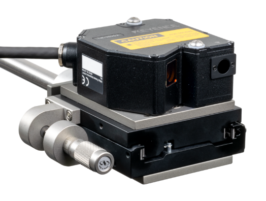
Mount the Translation Stage (11) on the laser bracket (8). Then mount the laser platform (7) on the Translation Stage (11) and mount the laser head to the platform using screws (10) and washers (9). Screw the laser rod (7) into the laser bracket (8).

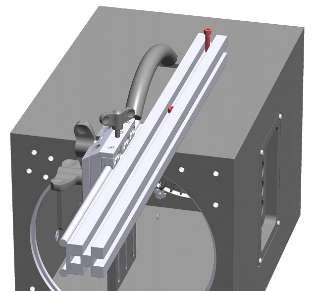
Mount the laser rack (3) to the LST Box (2) using Allen screws (4) and discs (5).

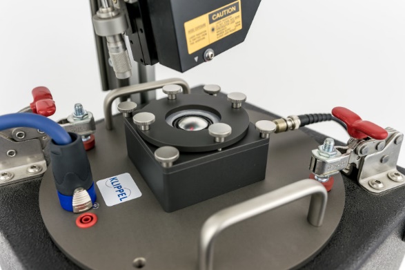
Place the MSPM bench (1) on the LST Box (2). Connect the MSPM bench (1) to terminal SPEAKER 1 of the Distortion Analyzer or Klippel Analyzer 3 Speaker-Card by using the speaker cable (12). Insert and connect the microphone (15).

Mount the laser rod including the laser platform and sensor to the rack.

MSPM Bench + Pro Driver Stand#

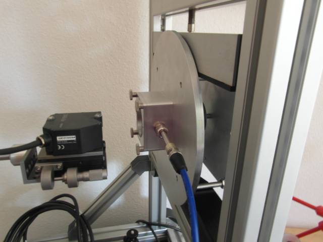
Clamp the MSPM Bench on the screws between the platforms or on the lower platform into the Pro Driver Stand.

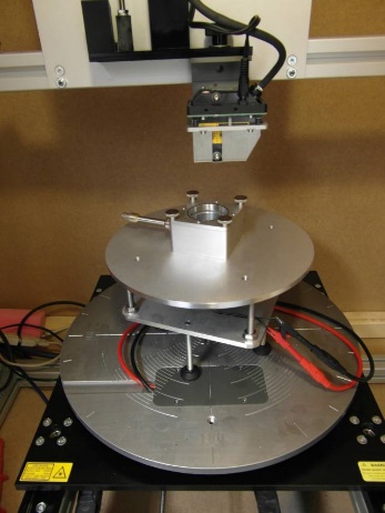
MSPM Bench + Laser Scanner#

Place the MSPM Bench on the laser scanner platform and adjust the laser head.

Setting up the System#

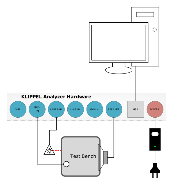
Connect the components in the following way:

For external amplifier: the output OUT1 of the analyzer device providing the stimulus signal is connected to the input of the power amplifier.
The output of the power amplifier or amplifier card is connected to the amplifier input of the Distortion Analyzer or Speaker-Card.
The laser displacement sensor is connected to the laser input of the analyzer device.
The microphone is connected to the microphone connector of the analyzer device.
The output SPEAKER 1 of the measurement device is connected to the work bench input.

For further details, see the KLIPPEL Analyzer Hardware.

MSPM Tutorial#

What is the Goal of This Tutorial?#

The tutorial gives step-by-step instructions on how to operate the micro suspension part measurement. (MSPM).

Tutorial 1 – Viewing Results: The first part Tutorial 1 – Viewing Results introduces the way the results are presented on the basis of the web example database.
Tutorial 2 – Performing a Measurement of the Linear Parameters (MSPM Lite): The second part Tutorial 2 – Performing a Measurement of the Linear Parameters (MSPM Lite) describes how to measure the stiffness and other parameters in the small signal domain.
Tutorial 3 – Performing a Measurement of the Nonlinear Stiffness K(x) (MSPM Pro): The third part Tutorial 3 – Performing a Measurement of the Nonlinear Stiffness K(x) (MSPM Pro) describes how to measure the large signal behavior of the DUT.
Tutorial 4 – Verification and Interpretation of the Results (MSPM Pro): The fourth part Tutorial 4 – Verification and Interpretation of the Results (MSPM Pro) explains the different output windows of the MSPM Pro and provides easy ways to verify the displayed results and to detect errors.

Tutorial 1 – Viewing Results#

Example data used in this manual is stored in the Web Example database. If not downloaded already, get it from the latest R&D release <https://www.klippel.de/go/current-rnd-release> and open the web-based database.

MSPM Lite#

Open the operation 1 MSPM Lite Micro SPM and the window Results.

The output table shows the calculated linear parameters. The resonance frequency \(f_{\text{r}}\) and the quality factor \(Q\) are directly derived from the measured transfer functions. The complete set of linear parameters is calculated by the Added Mass Method or by the given moving mass.

MSPM Pro#

Open the operation 2 MSPM Pro Micro SPM and the result window K(x) Stiffness.

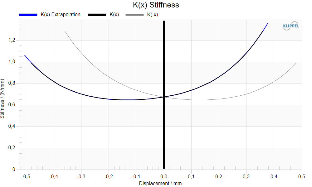
The black curve shows the stiffness over displacement in the working range (-0,48 mm \(< x <\) +0,36 mm).

Nonlinear Stiffness K(x)#

In contrast to the linear model the stiffness of a real sample is not constant but varies with displacement \(x\). Thus, the stiffness \(K(x)\) versus displacement reveals the nonlinearity of the micro speaker membrane. The \(K(x)\) measured on the micro speaker in the diagram above shows that the stiffness at the positive displacement \(x =\) 0,36 mm is higher than at the rest position. There is also a distinct asymmetry in the curve. Under dynamic operation an AC-signal is partially rectified and a negative DC-component is generated.

Tutorial 2 – Performing a Measurement of the Linear Parameters (MSPM Lite)#

Measurement procedure:

Preparing the DUT
Preparing the Measurement Setup
Setting Up the MSPM Lite Module
Starting the Measurement
Adding Mass to the DUT
Checking the Results
Using Advanced Parameters

Preparing the DUT#

In most cases, the DUT needs to be glued onto a stiff plate with dimensions of 55 mm by 55 mm. (e.g. PCB material). Although the used technique can cope with significant air porosity of the DUT material, the joint should be as sealed as possible due to the pneumatic excitation and the high sound pressures required.

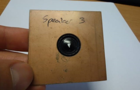
The forming and gluing of the membranes influence the results significantly. It should be homogeneous and reproducible to get reliable and reproducible data.

Note

In contrast to the normal operation of micro speaker diaphragms where the force excitation is ringlike due to the voice coil, in this method the membrane is excited over the whole surface by the sound pressure. To come closer to the final application a coil could be glued to the DUT before measuring it with the MSPM.

Preparing the Measurement Setup#

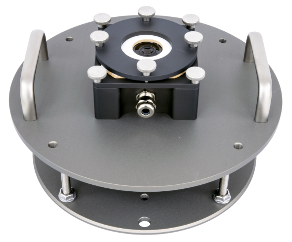
Unscrew the clamping ring from the enclosure. Place the DUT on the platform.

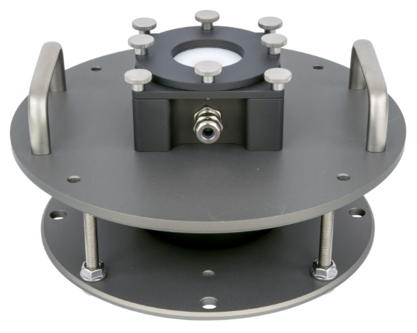
Fix the DUT between the two mounting parts using the 4 screws.

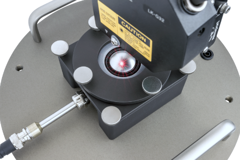
Direct the laser beam to the center of the membrane. Potentially a white dot is needed on the membrane for proper reflection. Adjust the laser position so that the laser is in its center position.

Setting Up the MSPM Lite Module#

The goal of this section is to explain how to set up the MSPM Lite Module. The MSPM Module creates the required TRF operations and automatically adjusts the stimulus.

Start db-Lab and create a new object using the object template MSPM Pro Micro Suspension Part Measurement.

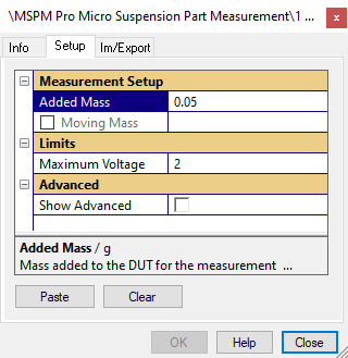
Open the Property Page SETUP. Set either the known moving mass of the DUT or the additional mass which will be used for the Added Mass Method.

Note

Entering the microphone sensitivity is not required anymore since it will be inherited automatically from global dB-Lab setting.

Starting the Measurement#

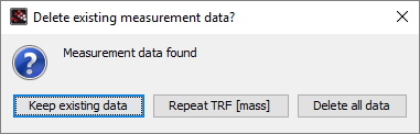
Message boxes guide you through the different measurement steps. The depicted message box is only shown if the module is run a second time and measurement data already exist.

Keep existing data: Keep existing data will process the previous TRF – Transfer Function Measurement operations. Use this if you have changed a post processing parameter (\(f_{\text{min}}\) fitting, \(f_{\text{max}}\) fitting) or if you have performed a TRF manually.
Repeat TRF [mass]: Repeat TRF [mass] can be used if another added mass is more suitable for this DUT. This step will keep the measurement without mass.
Delete all data: Delete all data repeats all necessary measurements and deletes previous result data.

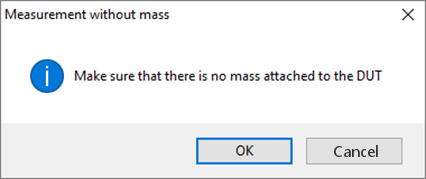
If running the module for the first time or choosing Delete all data in the previous step a message box asks you to start the measurement without mass. The TRF – Transfer Function Measurement operation is generated automatically and run several times until the best stimulus is found.

Adding Mass to the DUT#

If the moving mass of the DUT is not known, the Added Mass Method is needed for the full set of linear parameters.

If the parameter Moving mass is unchecked or empty and an Added Mass is given in the input page you are now asked to add a known mass to the DUT.

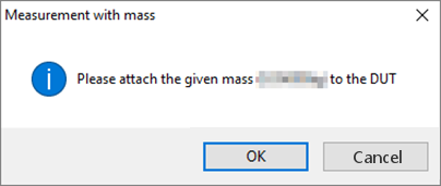
It is practical to use weighed putty as added mass. The mass should have a weight of around 50 % to 100 % of the diaphragm.

Place the additional mass on the diaphragm, carefully. It is useful to attach the mass on the bottom side of the diaphragm if the top side is sprayed with coating spray.

Place the mass at the potential voice coil position, to ensure conditions close to the final application. Especially for very thin/soft membranes, the measured parameters may change, if the added mass is attached in the center only.

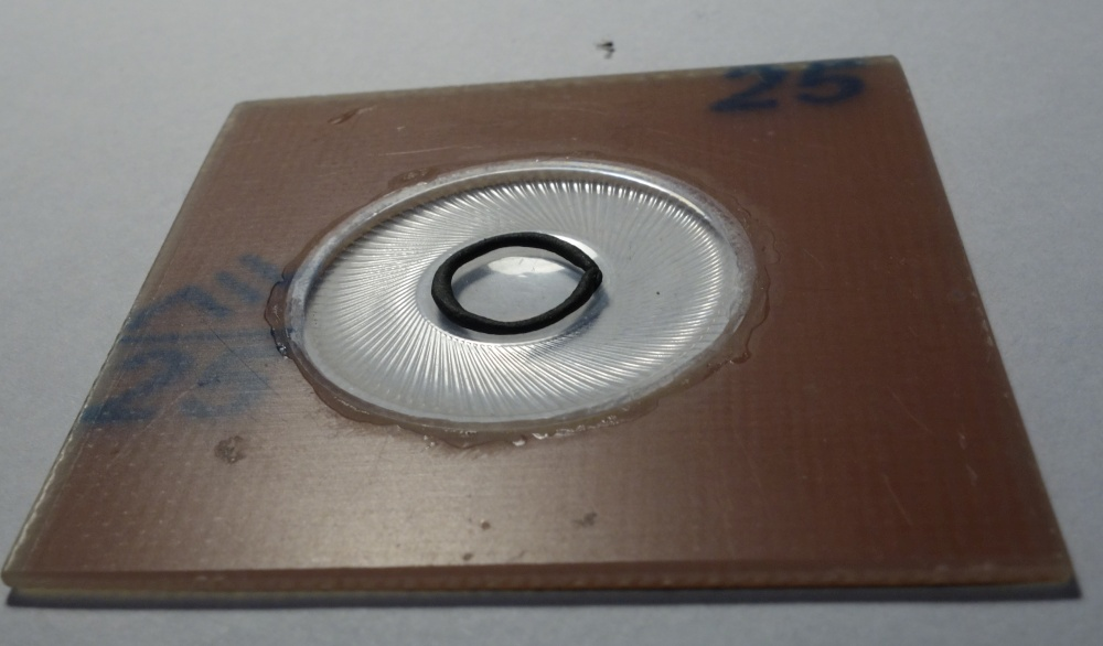
After pressing Run the TRF – Transfer Function Measurement operation is generated automatically and run several times until the best stimulus with the required target displacement is found.

Checking the Results#

When the TRF measurements are finished, the parameters are calculated and displayed.

The db-Lab object now contains the two TRF – Transfer Function Measurement operations holding the measurement data and the MSPM Lite module with the results.

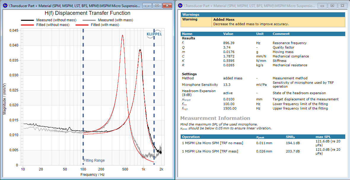
In the left window the extracted transfer functions between displacement and sound pressure are displayed. The mean fitted curves should match the measured curves around resonance.

The right window shows the calculated output parameters, errors and warnings, and information about the TRF – Transfer Function Measurement operations.

How to act in case of errors or warnings is explained in a later section in this manual.

To verify the correctness of the calculated parameters it is advised to take a closer look to the additional information table.

The maximum displacement of the DUT should be clearly in the linear domain. Good limits are a x peak value below 0.05 mm and a SNR around 30 dB. Changing the target displacement is explained in the next section.

Additionally, the maximum sound pressure level should be within the working range of the microphone.

Using Advanced Parameters#

Advanced parameters can be used to tune the performance of the MSPM. Activate Show Advanced checkbox to show all advanced parameters.

Target x: Unit: mm

This parameter defines the target displacement for linear vibration of the DUT. You can lower this value if the SNR is far better than 30 dB for example.
Start Voltage: Unit: V

With this value you can speed up the stimulus targeting. Set this value to the approximate end stimulus voltage based on earlier measurements.
fLow / fHigh Fitting: Unit: Hz

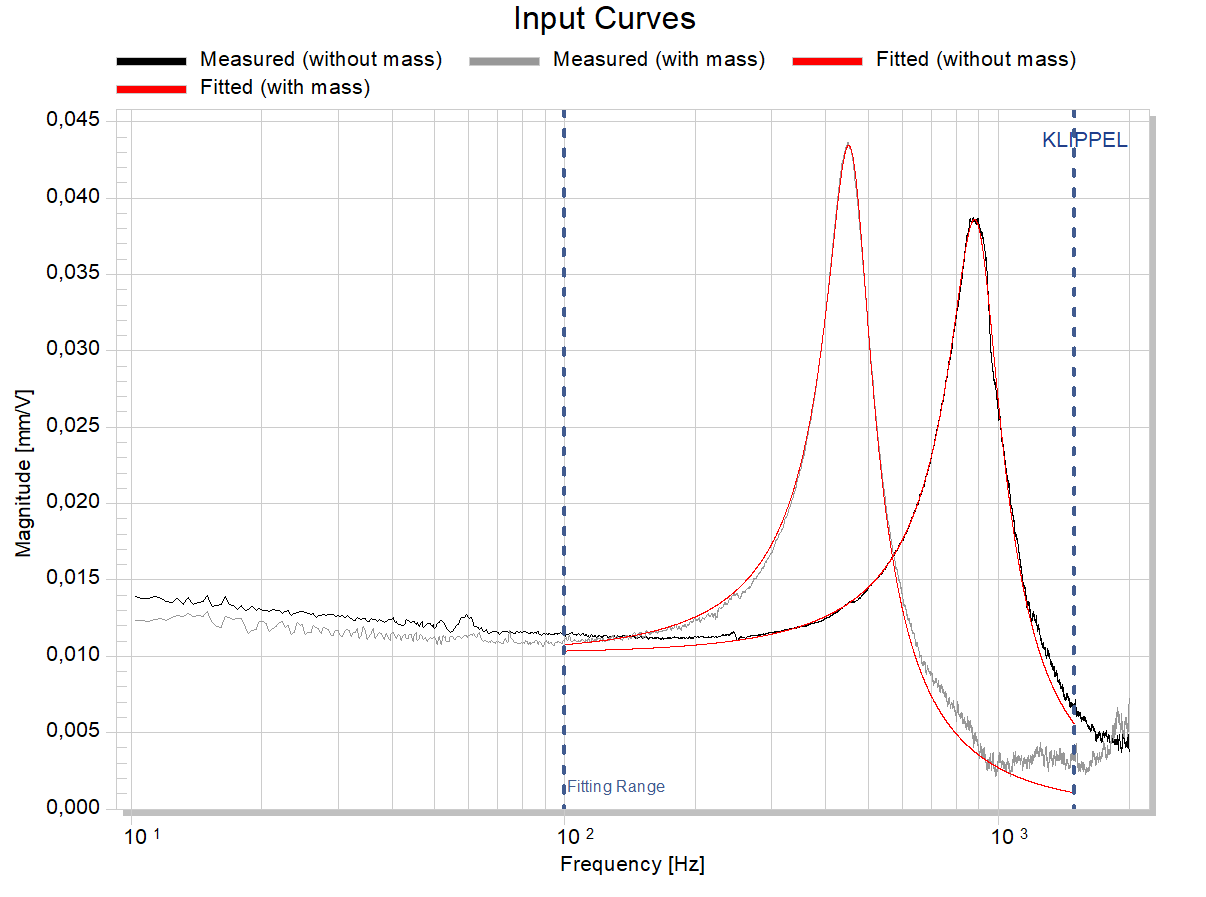
These parameters determine the bandwidth used for the parameter fitting. In the result window H(f) Displacement Transfer Function the parameters are indicated by the dashed vertical lines. Adjust these values if the resonance peaks are not within the lines or if there are low or high frequency disturbances which are higher than the resonance peak.

Tutorial 3 – Performing a Measurement of the Nonlinear Stiffness K(x) (MSPM Pro)#

Measurement procedure:

Preparing the DUT and the Measurement Setup
Setting Up the MSPM Pro Module
Starting the Measurement
Checking the Results
Using Advanced Parameters

Preparing the DUT and the Measurement Setup#

Prepare the DUT and the measurement setup as described in Tutorial 2 – Performing a Measurement of the Linear Parameters (MSPM Lite). If you have done the linear measurement before, leave the setup as it is.

Setting Up the MSPM Pro Module#

The goal of this section is to explain how to set up the MSPM Pro Module. The MSPM Module creates the necessary LPM operations and automatically adjusts the stimulus.

Start db-Lab and create a new object using the object template MSPM Pro.

Skip this step if you have already created this object for the linear measurement.

Note

The MSPM Pro needs a set of linear parameters for the calculation of the nonlinear stiffness. Therefore, it is recommended to perform the MSPM Lite first to get the linear parameters with the same measurement setup. For this reason, the combined template MSPM Pro is recommended.

Open the Property Page Setup. Required input parameters are in the categories Input and Limits.

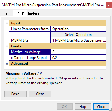
Maximum Voltage: The Maximum Voltage limits the maximum applicable stimulus voltage.

Warning

Caution! Consider the voltage limit of the driving speaker! See the specifications available on the MSPM module website for details.

X Target – Large Signal: X Target – Large Signal defines the desired working range in which the nonlinear stiffness of the DUT should be measured.
Select operation: The Select operation button allows to choose the previously performed MSPM Lite operation as source for the linear parameters.

Starting the Measurement#

Click Run to start the MSPM Pro measurement.

Message boxes guide you through the different measurement steps.

The message box is only shown if the module is run a second time and previous LPM already exist.

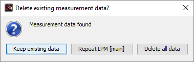
Keep existing data: Keep existing data will process the previously measured data. Use this if you have changed a post processing parameter (fLow Fitting, fHigh Fitting) or if you have performed a manual LPM measurement.
Repeat LPM [main]: Repeat LPM [main] repeats the main LPM operation. This is helpful if you have not reached any of your measurement limits in a previous run.
Delete all data: Delete all data repeats all necessary measurements and deletes previous LPM operations.

If no previous data is existing a message box asks you to start the measurement.

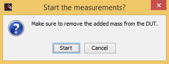
The LPM operations are generated automatically and run several times until the right stimulus is found.

The stimulus automation starts with the reference LPM and goes on with the main LPM in the large signal domain.

Checking the Results#

When the LPM measurements are finished the script starts the parameter calculation and afterwards the results are shown.

The db-Lab object now contains the two LPM operations holding the measurement data and the MSPM Pro module with the results.

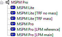
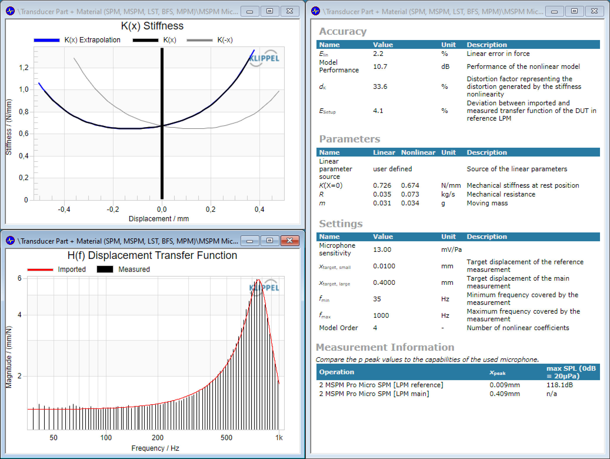
The upper left window shows the calculated stiffness over displacement. The lower left window shows the imported and measured linear transfer function. The window can be used to assess deviations in the setup of the MSPM Lite and MSPM Pro.

In the Overview window the result parameters are displayed. To verify the validity of the fitted result curves, it is recommended to check the fitting errors first:

\(E_{\text{lin}}\): \(E_{\text{lin}}\) reflects the fitting error considering linear model parameters. It should be below 10 %.
Model Performance: Model performance reflects the quality of the nonlinear model fitting; a high level is desirable here
\(E_{\text{Setup}}\): \(E_{\text{Setup}}\) considers some model assumptions and should be below 10 %, ideally. This error is calculated based on the deviation between the transfer function of the DUT calculated by the imported parameters and the measured transfer function with the reference LPM. These transfer functions are shown in the window H(f) Force Transfer Function and H(f) Displacement Transfer Function.

How to act in case of errors or warnings is explained in a later section in this manual.

Using Advanced Parameters#

Advanced parameters are initialized with default values and can be adjusted to improve performance in some cases.

x Target – Small Signal: This parameter determines the target displacement for linear vibration in mm. Adapt this value if the distortion level in the reference LPM is too high or the SNR is too low (indicated by an error message).
Start Voltage Ref LPM: With this value you can speed up the stimulus automation. Set this value to the approximate end stimulus voltage of former measurements.
Start Voltage Main LPM: see above
f min / f max: These parameters determine the bandwidth for the parameter fitting. F min removes low frequency range where the deviation between modeled and measured transfer functions of the DUT is usually high. If left empty it is automatically determined.

A possible reason for restricting f max is explained in the next section.
Model Order: This is the number of nonlinear coefficients for the stiffness power series expansion:

\[K(x) = k_{0} + x \cdot k_{1} + x^{2} \cdot k_{2} + x^{3} \cdot k_{3} + \ldots\]

Tutorial 4 – Verification and Interpretation of the Results (MSPM Pro)#

The goal of this tutorial is to provide methods to verify the calculated results from the MSPM Pro and to interpret the output windows which are not described in the previous tutorial.

Open the web example database described in the first tutorial or use the database from the tutorial 3.

Verification by Multiple Measurements#

In general, the best verification of a measurement is repeating the measurement at multiple laser target points on the DUT surface. The results should correlate for all measurements. The points used should be close to the position at which the voice coil is mounted, as this is the position at which the force is induced in the final application of the loudspeaker membrane.

The Different Error Values#

As described in the last section there are three error values to check the validity of the results. Additional graphs which are the base for those numbers provide further diagnostic information.

E Lin#

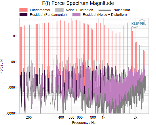
Open the window F(f) Force Spectrum.

This linear error is based on the spectrum of the exciting force inside the enclosure (Fundamental) and the remaining error at the excited frequencies (Residual (Fundamental)) that cannot be explained by the model.

Important here is that the fundamental error lines about the same level as the error lines off the fundamental frequencies. In combined with a high value in Model Performance, the accuracy of the linear part of the model (e.g., \(K(x = 0)\)) is high.

Model Performance#

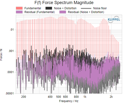
Open the window F(f) Force Spectrum.

The Model Performance reflects the ratio of the measured distortion (Noise + Distortion) which is the base for the nonlinear fitting vs. the remaining distortion (Residual (Noise + Distortion)) after the fitting that cannot be explained by the nonlinear model.

In case of successful measurement and fitting, the grey Noise + Distortion curve must be above the Residual (Noise + Distortion)) which is reflected by a Model Performance value \(>\) 0.

Values close to or below zero indicate invalid results. If there is no big difference between the two curves above a certain frequency, fHigh can be adjusted to this frequency to use a smaller frequency range and reduce the resulting errors.

E Setup#

For the MSPM Pro measurement method, some model assumptions have to be made which can be checked by the setup error value.

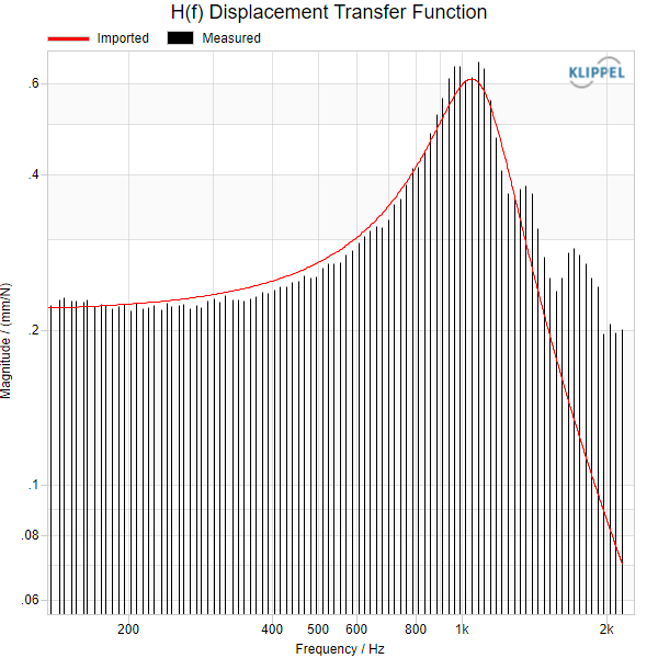
The window H(f) Force Transfer Function can be used to check the validity of the imported linear parameters. This window was already explained in tutorial 3.

Open H(f) Displacement Transfer Function. This window shows the modeled transfer function of the measurement setup which is determined by the measured curves from the reference LPM and the imported linear parameters. The agreement of the modeled and the measured transfer function can be checked here.

MSPM - Reference#

MSPM Lite#

The MSPM Lite is used to measure the linear mechanical parameters of small suspension parts.

Measurement Technique#

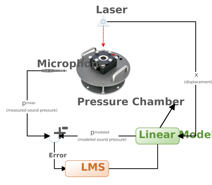
The DUT is excited by the sound pressure in a small pressure chamber generated by an integrated transducer. The sound pressure inside the pressure chamber is measured with a microphone and the displacement of the DUT is measured with a laser sensor. Then the transfer function from sound pressure to displacement is calculated.

This transfer function is modeled with a spring mass system and fitted to the measured transfer function, deriving the resonance frequency and the quality factor. The linear parameters are determined by the measurement of the resonance shift when adding a known mass (Added Mass Method) or by calculating it from the known moving mass of the DUT.

Property Page#

Category Measurement Setup#

The Measurement Setup category contains parameters that define the measurement conditions.

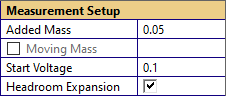
Added mass: Unit: g

Range: \(0 < M_{\text{add}}\)

Mass added to the DUT for the measurement with mass. This value is not required if the moving mass of the DUT known.
Moving mass: Unit: g

Range: \(0 < M_{\text{ms}}\)

Known moving mass of the DUT. If not known use the Added Mass Method.
Start Voltage: Unit: V

Range: \(0 < U_{\text{start}}\)

Initial stimulus voltage for the TRF – Transfer Function Measurement stimulus automation.

Note

Only displayed if Show advanced is selected.
Headroom Expansion: If activated, an 8 dB Headroom Expansion is used for the TRF – Transfer Function Measurement measurement. Deactivate this parameter if you experience bad SNR in the sound pressure signal.

Category Limits#

This parameter category defines the maximum allowed limits of the measurement. If one of these criteria is reached, the measurement is stopped automatically.

Maximum Voltage: Unit: V

Range: \(0 < U_{\text{max}} \leq 2\)

Voltage limit for the TRF operations used by the stimulus automation. This value must be in the working range of the driving speaker. See the specifications available on the MSPM module website for details. Note: Only displayed if Show advanced is checked
Target X: Unit: mm

Range: \(x_{\text{target}} > 0\)

Target displacement of the DUT for linear vibration.

Category Processing#

The category Processing defines parameters which will affect the fitting of the measurement data. Changing these parameters will affect your results.

Note

The following parameters are only shown if Show advanced is activated.

fLow Fitting: Unit: Hz

Range: 0 \(< f_{\text{low}} < f_{\text{high}}\)

Cutoff frequency of the high-pass filter. Limits lower fitting range in order to remove disturbances like the influence of leakage.
fHigh Fitting: Unit: Hz

Range: \(f_{\text{low}} < f_{\text{high}}\)

Cut-off frequency of the low-pass filter. Limits upper fitting range in order to remove disturbances like the influence of noise.

Category Advanced#

By activating Show Advanced, additional parameters are displayed.

Results#

Parameters#

Those parameters are calculated from the measurement data and can be exported to the clipboard for further computation.

\(M_{\text{ms}}\): Moving mass
\(K_{\text{ms}}\): Mechanical stiffness of suspension
\(R_{\mathrm{ms}}\): Mechanical resistance due to losses

Result Windows#

Input Curves#

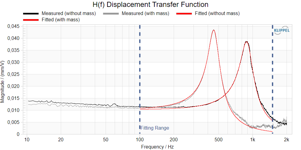
Imported transfer functions with and without mass and their mean fitting curves. This window also shows the fitting range (\(f_{\text{low}}\) , \(f_{\text{high}}\)). Check this window for good fitting or frequency regions of bad fitting.

Table Results#

\(f_{\text{r}}\): Resonance frequency
\(Q\): Quality factor
\(m\): Moving mass
\(C\): Mechanical compliance of the suspension
\(K\): Mechanical stiffness of the suspension
\(R\): Mechanical resistance due to mechanical losses

MSPM Pro#

The MSPM Pro is used to measure the nonlinear mechanical stiffness characteristic of a micro suspension.

Measurement Technique#

The DUT is excited by the sound pressure of a small pressure chamber. The displacement of the DUT is measured with a laser sensor and the driving force \(F_{\text{Stim}}\) is anticipated by the measurement of the current of the driving speaker, and knowing the transfer function \(H_{\text{Setup}}\) from current to force.

The algorithm fits the nonlinear model, by minimizing the error between the anticipated force \(F_{\text{Stim}}\) and the modeled force \(F_{\text{Model}}\). Inside the pressure chamber, the force \(F\) is proportional to the sound pressure.

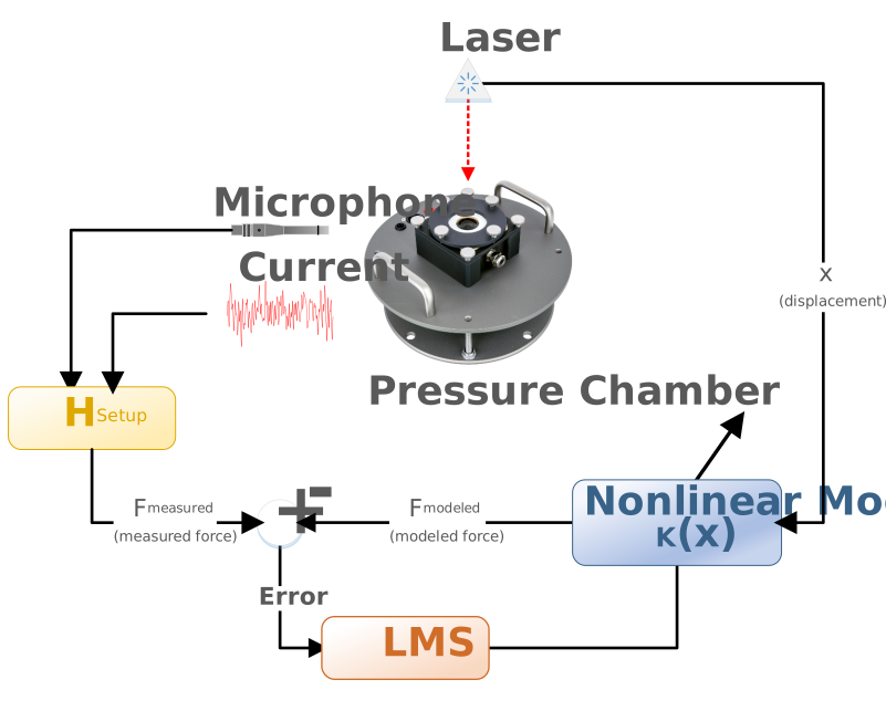
The MSPM Pro measurement is performed in 2 steps:

1. Reference measurement: In this measurement, the transfer function from current \(i\) to displacement \(x\) is measured in order to identify the transfer function \(H_{\text{Setup}}\). This measurement is done at very low stimulus level, so the nonlinear model of the DUT can be reduced to the linear model, as identified in the linear measurement. For verification purpose, also the sound pressure signal is measured in this step.

2. Main measurement: In this step, the stimulus is increased, to reach the target displacement of the DUT. As the sound pressure exceeds the limits of ordinary microphones, the pressure \(F_{\text{Stim}}\) inside the chamber is calculated from the current, using the transfer function \(H_{\text{Setup}}\).

Property Page#

Category Input#

Since the MSPM Pro is directly dependent on the MSPM Lite, it needs to either import or user specify the linear micro suspension part parameters.

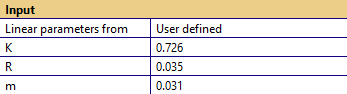
or

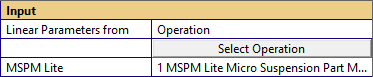
Linear parameters from: - User defined: manual insertion of parameters

- Operation: import linear parameters from a given MSPM Lite operation

Specify the source for the linear mechanical suspension part parameter.
\(K\): \(K\) in N/mm

Range: 0 \(< K_{\text{ms}}\)

Linear stiffness of the suspension part
\(R\): \(R\) in Kg/s

Range: 0 \(< R_{\text{ms}}\)

Linear mechanical resistance of the suspension part
\(m\): \(m\) in g

Range: 0 \(< M_{\text{ms}}\)

Linear moving mass of the suspension part

Category Measurement Setup#

The Measurement Setup category contains parameters that define the measurement conditions.

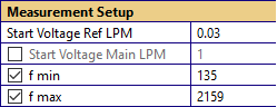
Start Voltage Ref LPM: \(U_{\text{start,ref}}\) in V

Range: \(0 < U_{\text{start,ref}}\)

Initial stimulus voltage for the LPM stimulus automation.

Note

Only displayed if Show advanced is checked.
Start Voltage Main LPM: \(U_{\text{start,main}}\) in V

Range: \(0 < U_{\text{start,main}}\)

Initial stimulus voltage for the main LPM stimulus automation. If unchecked, this value is calculated automatically.

Note

Only displayed if Show advanced is checked.
f min: \(f_{\text{min}}\) in Hz

Range: \(0 < f_{\text{min}}\)

Cut-off frequency of the high-pass filter. Limits fitting range to cut out disturbances like the influence of a leakage (automatically set if deactivated).
f max: \(f_{\text{max}}\) in Hz

Range: \(f_{\text{min}} < f_{\text{max}}\)

Cut-off frequency of the low-pass filter. Limits fitting range to cut out disturbances like the influence of noise. Distortions up to this limit are used for the curve fitting.

Category Limits#

Defines the maximum allowed limits of the measurement. If one of these criteria is reached, the measurement is stopped automatically.

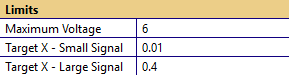
Maximum Voltage: \(U_{\text{max}}\) in V

Range: \(0 < U_{\text{max}}\)

Stimulus voltage limit for the automated displacement targeting. This value must be within the working range of the driving speaker. See the specifications available on the MSPM module website for details.
Target X – Small Signal: \(x_{\text{target, small}}\) in mm

Range: \(0 < x_{\text{target, small}}\)

Target displacement for linear vibration. If deactivated, target displacement from the linked MSPM Lite is used. Note: Only displayed if Show advanced is activated.
Target X – Large Signal: \(x_{\text{target,large}}\) in mm

Range: \(0 < x_{\text{target,large}}\)

Desired maximum displacement amplitude of the DUT. The stimulus is adjusted in order to reach this peak value.

Category Processing#

The category Processing defines parameters which will affect the fitting of the measurement data. Changing these parameters will affect your results.

Note

This category is only shown if Show advanced is selected.

Model Order

Number of power series coefficients for the nonlinear curve fitting.

2^nd order
4^th order

Category Advanced#

By selecting Show Advanced, additional measurement options are displayed.

Results#

Parameters#

Those parameters are calculated from the measurement data and can be exported to the clipboard for further computation.

\(K_{\text{ms}}\): Mechanical stiffness of micro suspension
\(k_{1} \text{...} k_{4}\): Coefficients of the nonlinear stiffness power series expansion. The number of coefficients depends on Model Order.
\(M_{\text{ms,part}}\): Moving mass of micro suspension
\(R_{\text{ms,part}}\): Mechanical resistance due to mechanical losses of micro suspension

Result Windows#

K(x) Stiffness#

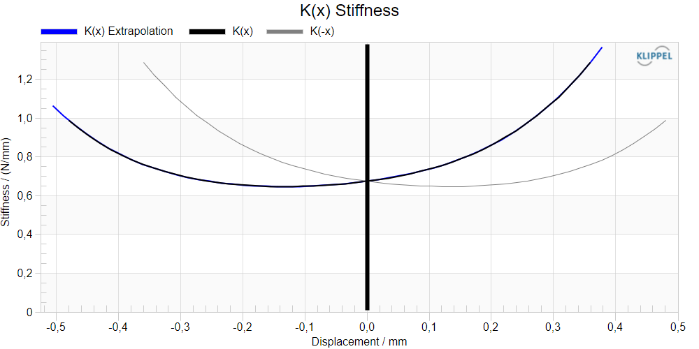
The window shows the identified nonlinear stiffness \(K(x)\) of the micro suspension part. The curve based on a (regular) power series following the form

\[K(x) = k_{0} + x \cdot k_{1} + x^{2} \cdot k_{2} + x^{3} \cdot k_{3} + \ldots\]

K(x) Extrapolation curve: up to 100 % of the reached displacement
K(x) curve: up to 90 % of the reached displacement
K(-x) curve: mirrored \(K(x)\) at rest position

F(f) Force Spectrum#

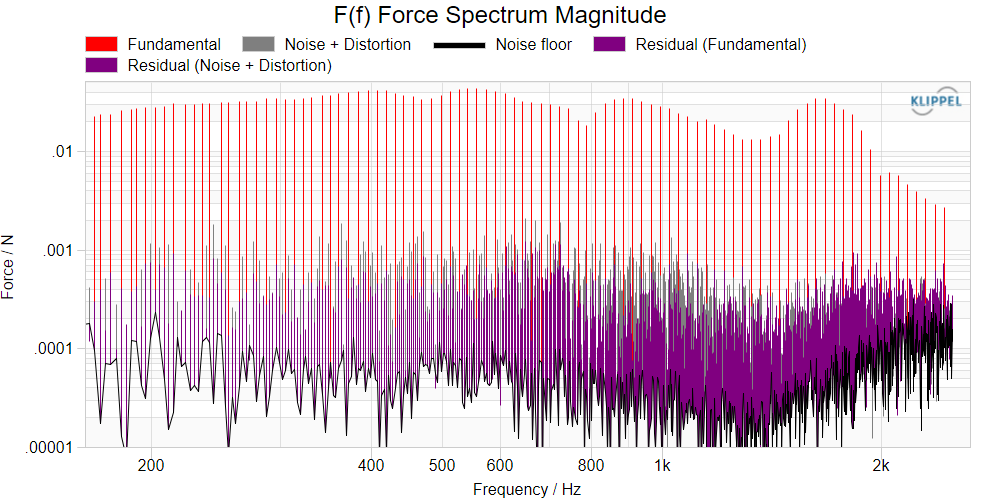
This is a diagnostics window that shows the forces \(F\) in the frequency domain. You can use this plot to check fitting performance of both linear and nonlinear parameters.

Displayed are

the Fundamental component, representing the excited frequency lines,
Noise + Distortions, representing the signal above noise floor on the non-excited frequencies,
Noise Floor, representing the measured noise floor of the measurement,
Residual (Fundamental), the remaining signal after the linear modeled force is subtracted, and
Residual (Noise + Distortion), the remaining after the nonlinear modeled force is subtracted.

The Fundamental spectrum is calculated from the current signal \(i(t)\) of the driving speaker, transformed to the force domain. All other spectra are calculated based on the measured displacement signal \(x(t)\).

A good linear fitting is performed if the purple curve Residual (Fundamental) is sufficiently lower than the fundamental. A good nonlinear fitting is performed if the curve Residual (Noise + Distortions) is sufficiently lower than the fundamental.

H(f) Displacement Transfer Function#

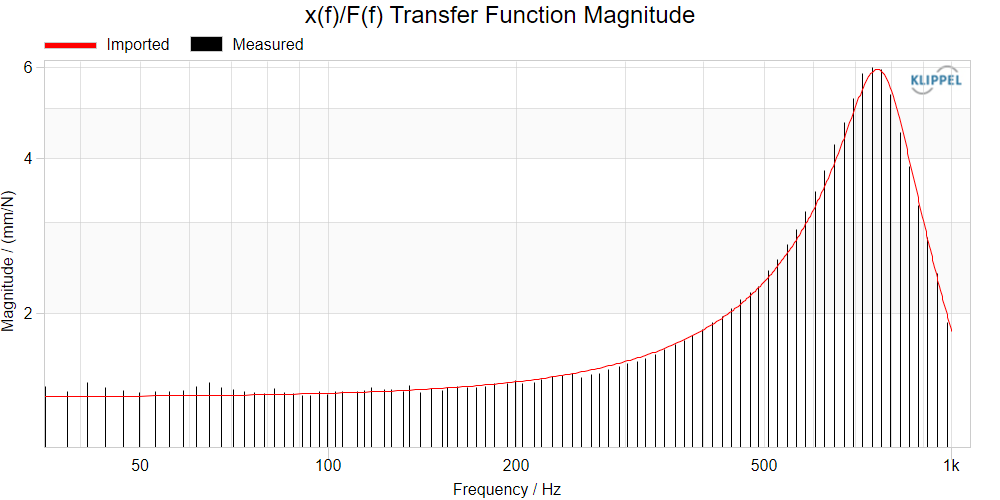
This is a diagnostics window that shows the transfer function between force and displacement of the DUT. The black curve shows the result of the reference measurement, the red curve the transfer function calculated from the linear parameters (imported / provided by the user).

Both curves should match well.

H(f) Force Transfer Function#

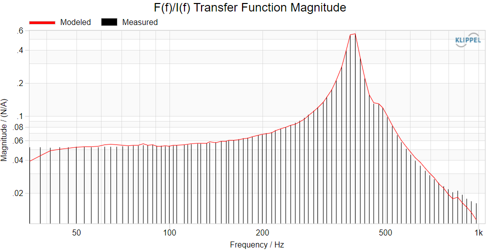
This is a diagnostics window that shows the transfer function between current and force. The black curve is the result of the reference measurement, the red curve the transfer function calculated from the linear parameters (import / provided by the user).

Both curves should match well.

Table Results#

Accuracy#

\(E_{\text{lin}}\): Unit: %

Linear error in force relative to stimulus signal \(F_{\text{Stim}}\). This is a pure linear error, representing the mismatch of the linear model only.
Model Performance: Unit: dB

Performance of the nonlinear model. Higher numbers represent better fitting of \(K(x)\). If the number gets negative, though the fitted curve may look convenient, the fitting failed.
\(d_{\text{K}}\): Unit: %

Ratio of the distortion in measured displacement, transformed into force domain
\(E_{\text{Setup}}\): Unit: %

Error in measured transfer function

Parameters#

\(K(x = 0)\): Unit: N/mm

Mechanical stiffness at rest position
\(R\): Unit: kg/s

Mechanical resistance
\(m\): Unit: g

Moving mass

Settings#

\(x_{\text{target,small}}\): Unit: mm

Target displacement for reference measurement
\(x_{\text{target,large}}\): Unit: mm

Target displacement for main measurement
\(f_{\text{min}}\): Unit: Hz

Minimum frequency covered by the measurement. Minimum frequency covered by the measurement.
\(f_{\text{high}}\): Unit: Hz

Maximum frequency covered by the measurement. Also used as upper frequency limit of fitting bandwidth.
Model Order: Order of series expansion used for parameter fitting

Supported Modules for Im/Export#

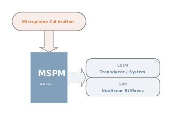
Malfunction and Troubleshooting#

Overview#

This chapter will provide information that can help you solve common problems that occur with MSPM (both Lite and Pro) measurements.

If you cannot find a description here that matches your problem, try these options:

Check the Malfunction and Troubleshooting section of the dB-Lab – Software documentation.
Check the file readme.txt that you received with your KLIPPEL products. This document contains the most up-to-date information about products and installation procedures.
Contact us via support.

Stimulus / Measurement (Automation)#

Error#

Measurement … aborted by user#

Cause: User pressed the Cancel button in the message box.
Recommended Action: Run the module again.

Information#

TRF/LPM iteration limit reached with … iterations.#

Cause: The target displacement could not be reached in a given number of steps.
Recommended Action: Check the laser adjustment. Check the surface of the DUT for proper laser reflection potentially a white dot is necessary on the DUT. Set a higher start voltage for the stimulus automation in the Advanced Settings.

\(u_{\text{max}}\) reached (…) but the displacement is below the target (…)#

Cause: The target displacement of the DUT could not be reached with the given voltage limit.
Recommended Action: Increase the voltage limit

Warning

Consider the voltage limit of the driving speaker! See the specifications available on the MSPM module website for details.

Low SNR (…)#

Cause: The signal to noise ratio in displacement is below the threshold.
Recommended Action: Increase the target displacement. Reduce environmental noise.

High distortion level (…)#

Cause: The distortion level in the reference LPM is too high (linear vibration is necessary).
Recommended Action: Reduce the target displacement for the small signal domain in the Advanced Settings.

MSPM Lite#

Error#

The resonance peak of Curve … was not determined correctly….#

Cause: The provided transfer function could not be fitted by the algorithm.
Recommended Action: Adjust the fitting range so that all resonance peaks are clearly within \(f_{\text{min}}\) and \(f_{\text{max}}\). Adjust the fitting range to cut out low or high frequency disturbances which are higher than the resonance peak. Check the stimulus automation for Low SNR warnings. Check that the laser sensor and the microphone provide reasonable data.

No results available.#

Cause: TRF exists but is empty.
Recommended Action: Make sure to run all necessary measurements. Use delete all data or Repeat TRF mass

The resonance frequencies with mass and without mass are identical.#

Cause: Both measurements are measured without (with) mass. The added mass is too small.
Recommended Action: Make sure to add a mass (only) for the measurement with mass. Increase the added mass.

The resonance frequency of the measurement with mass is higher than without mass.#

Cause: The measurements got mixed up. The resonance peaks are not clearly visible due to noise or other disturbances.
Recommended Action: Repeat the measurements in the correct order. The message boxes tell when to use the added mass. Adjust the fitting range to cut out disturbances which are higher than the resonance peak.

Warning

Increase the added mass to increase accuracy.

Cause: The resonance shift is too small.
Recommended Action: Increase the added mass.

Decrease the added mass to increase accuracy.#

Cause: The resonance shift is too high.
Recommended Action: Decrease the added mass.

MSPM Pro#

Warning

Low-cut is adjusted to the maximum allowed value for the automatic detection. …

Cause

There is a high deviation between the modeled transfer function of the setup and the control measurement with the reference LPM at low frequencies. This could be due to

a leaky enclosure/diaphragm
visco-elastic effects (creep) of the material

Recommended Action

Try to seal the area between DUT and mounting plate as good as possible. If the setup error is also very high due to this deviation try to increase the low-cut manually.

High setup error! (…)#

Cause: The modeled and measured transfer functions of the measurement setup do not fit. High error in the model assumptions.
Recommended Action: Check that the imported linear parameters belong to the measured DUT. Check for SNR or distortion level warnings of the reference LPM.

High fitting error!#

Cause: The residual error of the fitting algorithm is high. The measured data could not be explained by the model applied.
Recommended Action: Check that the laser sensor provides reasonable data. Check the measurement setup for proper cable connections. The reference and the main LPM should be executed in a reasonable working range.

MSPM – Micro Suspension Part Measurement

On this page

MSPM – Micro Suspension Part Measurement#

MSPM - Tutorial#

Overview#

MSPM Lite and MSPM Pro#

The Measurement Method#

MSPM Lite#

MSPM Pro#

MSPM Setup#

Overview#

Work Bench#

List of Parts#

Mounting Instructions#

MSPM Bench + LST Box#

MSPM Bench + Pro Driver Stand#

MSPM Bench + Laser Scanner#

Setting up the System#

MSPM Tutorial#

What is the Goal of This Tutorial?#

Tutorial 1 – Viewing Results#

MSPM Lite#

MSPM Pro#

Nonlinear Stiffness K(x)#

Tutorial 2 – Performing a Measurement of the Linear Parameters (MSPM Lite)#

Preparing the DUT#

Preparing the Measurement Setup#

Setting Up the MSPM Lite Module#

Starting the Measurement#

Adding Mass to the DUT#

Checking the Results#

Using Advanced Parameters#

Tutorial 3 – Performing a Measurement of the Nonlinear Stiffness K(x) (MSPM Pro)#

Preparing the DUT and the Measurement Setup#

Setting Up the MSPM Pro Module#

Starting the Measurement#

Checking the Results#

Using Advanced Parameters#

Tutorial 4 – Verification and Interpretation of the Results (MSPM Pro)#

Verification by Multiple Measurements#

The Different Error Values#

E Lin#

Model Performance#

E Setup#

MSPM - Reference#

MSPM Lite#

Measurement Technique#

Property Page#

Category Measurement Setup#

Category Limits#

Category Processing#

Category Advanced#

Results#

Parameters#

Result Windows#

Input Curves#

Table Results#

MSPM Pro#

Measurement Technique#

Property Page#

Category Input#

Category Measurement Setup#

Category Limits#

Category Processing#

Category Advanced#

Results#

Parameters#

Result Windows#

K(x) Stiffness#

F(f) Force Spectrum#

H(f) Displacement Transfer Function#

H(f) Force Transfer Function#

Table Results#

Accuracy#

Parameters#

Settings#

Supported Modules for Im/Export#

Malfunction and Troubleshooting#

Overview#

Stimulus / Measurement (Automation)#