
SPM – Suspension Part Measurement#
Overview#
SPM Lite and SPM Pro#
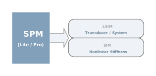
KLIPPEL SPM includes two modules for the measurement of medium and large size suspension parts (spiders, surrounds, cones).
The SPM Lite is dedicated to the measurement of the mechanical stiffness \(k_{0}\) in the small signal domain. In addition, the SPM Lite can be used to measure the linear parameters of passive radiators. Detailed instructions on measuring passive radiators are provided in Application Note 57.
The SPM Pro is additionally capable of measuring the nonlinear stiffness \(K(x)\) of suspension parts.
The Measurement Method#
SPM Pro#
The nonlinear stiffness \(k(x)\) and the reciprocal compliance \(C(x)\) of suspension parts and passive radiators (drones) are measured versus displacement \(x\) over the full range of operation. The Suspension Part Measurement (SPM) is a dynamic, nondestructive technique which excites the suspension parts pneumatically under similar condition as operated in the loudspeaker. The nonlinear parameters are estimated from the measured displacement signal. This guarantees highest precision of the results as well as simple handling and short measurement time. Suspension Parts below 220 mm diameter can be measured with the one-signal method [1].
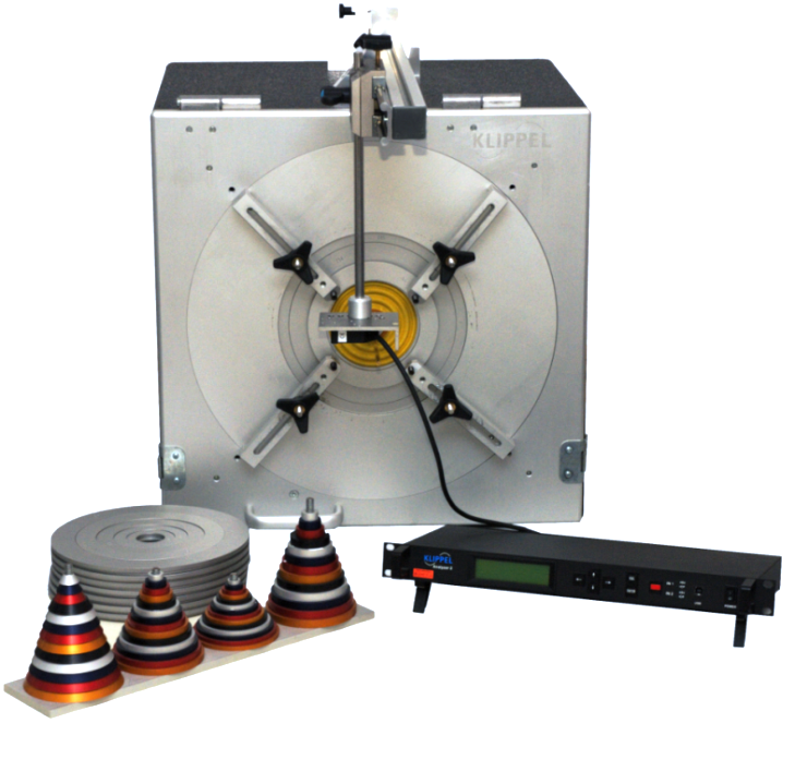
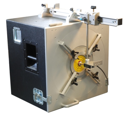
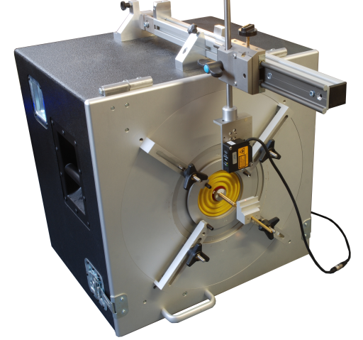
The picture below shows the SPM Pro test enclosure (SPM bench) with the working bench, a Distortion Analyzer, laser and clamping set. The working bench is equipped with an 18’’ subwoofer producing ± 20 mm displacement at low distortion. The box has an effective air volume of 95 liters.
The displacement sensor is directly mounted on the test box to minimize vibration, offset and other errors. The test box also provides an inlet for the optional microphone. Both sensors are powered by the measurement device. This platform also generates the stimulus provided via a power amplifier to the loudspeaker. The TRF – Transfer Function Measurement generates the sinusoidal sweep and measures displacement. The SPM module controls the measurement and calculates the results.
SPM Lite#
The measurement principle of the SPM Lite is comparable to the SPM Pro but it focuses on accurate measurement of linear parameters in the small signal domain only. Analyzing the transfer function, which is based on the simultaneous measurement of sound pressure and displacement, resonance frequency \(f_{\mathrm{s}}\) and \(Q\)-factor of the device under test are determined. By measuring the moving mass, using the Added Mass Method or a high precision scale, the complete set of linear parameters is calculated.
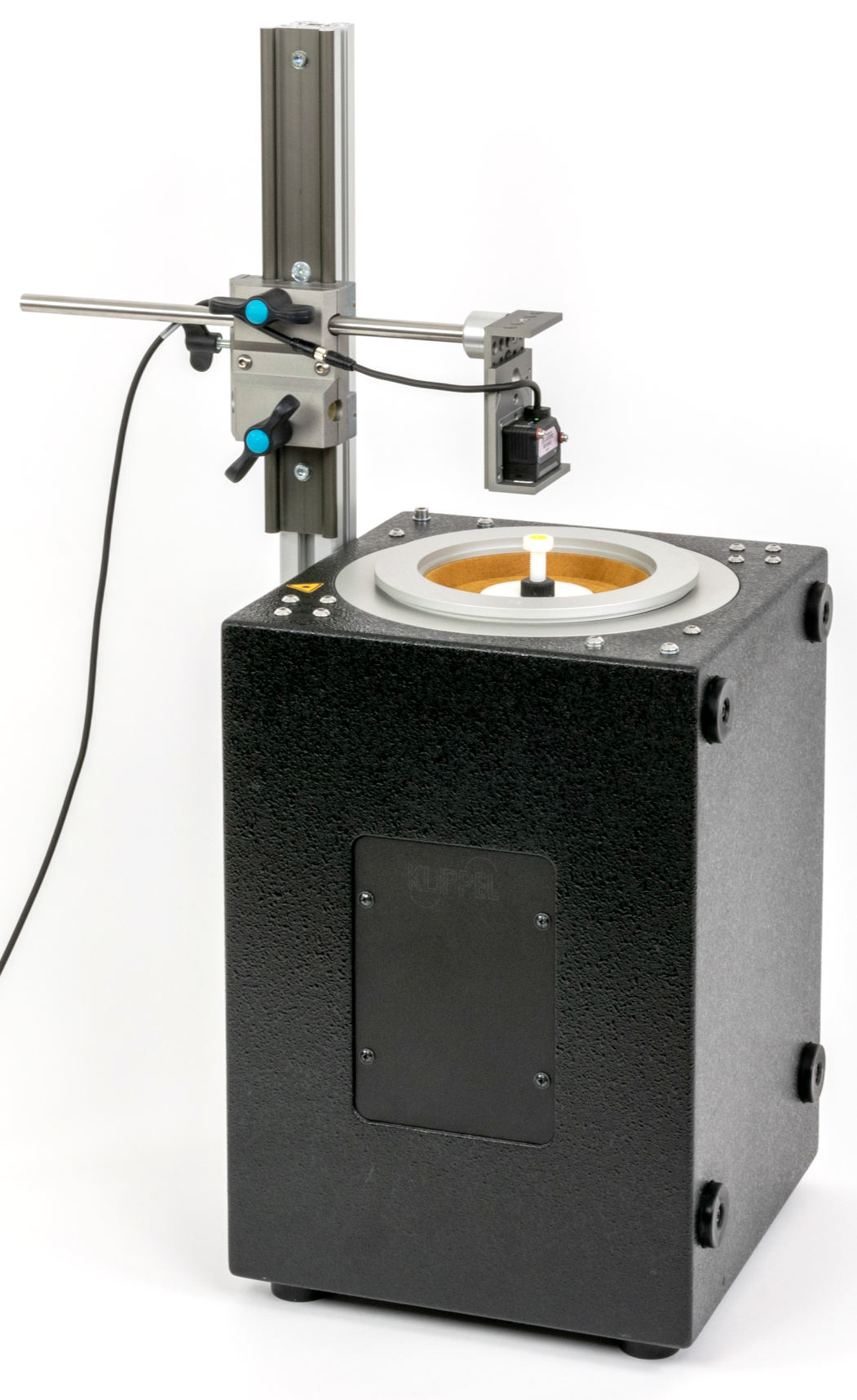
SPM Lite may be operated with the SPM Bench or the LST Bench with external boom (shown below). The LST measurement bench consists of a sealed enclosure with a volume of 9 liters and a 10” driver, which excites the device under test pneumatically. It provides an external rack for mounting the laser displacement sensor. The clamping platform is compatible to the SPM Ring Set. Both vertical and horizontal operation is provided by the test bench (additional clampers are supplied).
SPM Setup#
Overview#
Step-by-step instructions are provided to setup the hardware of the Suspension Part Measurement for the first time. It is assumed that the measurement bench is in the original packaging provided by the manufacturer. Please find additional instructions for installing the dB-Lab – Software and general information about the KLIPPEL Analyzer hardware and accessories in other parts of the manual.
The setup uses the following components:
work bench for pneumatic excitation of the suspension part
clamping parts (cone, cup, rings)
Measurement hardware (Distortion Analyzer hardware (DA2) or KLIPPEL Analyzer 3 (KA3))
amplifier + XLR cable
amplifier cable with speakON connector
SPM speaker cable (extra-long with two speakON connectors)
laser displacement sensor (e.g. laser head ANR 1282 + controller ANR 5132)
microphone (only necessary for the linear parameter measurement)
TRF – Transfer Function Measurement software module
SPM Lite software module
SPM Pro software module
Work Bench#
List of Parts#
SPM Bench#
- 1 Work bench
- Units: 1
driver mounted in enclosure, clamping platform
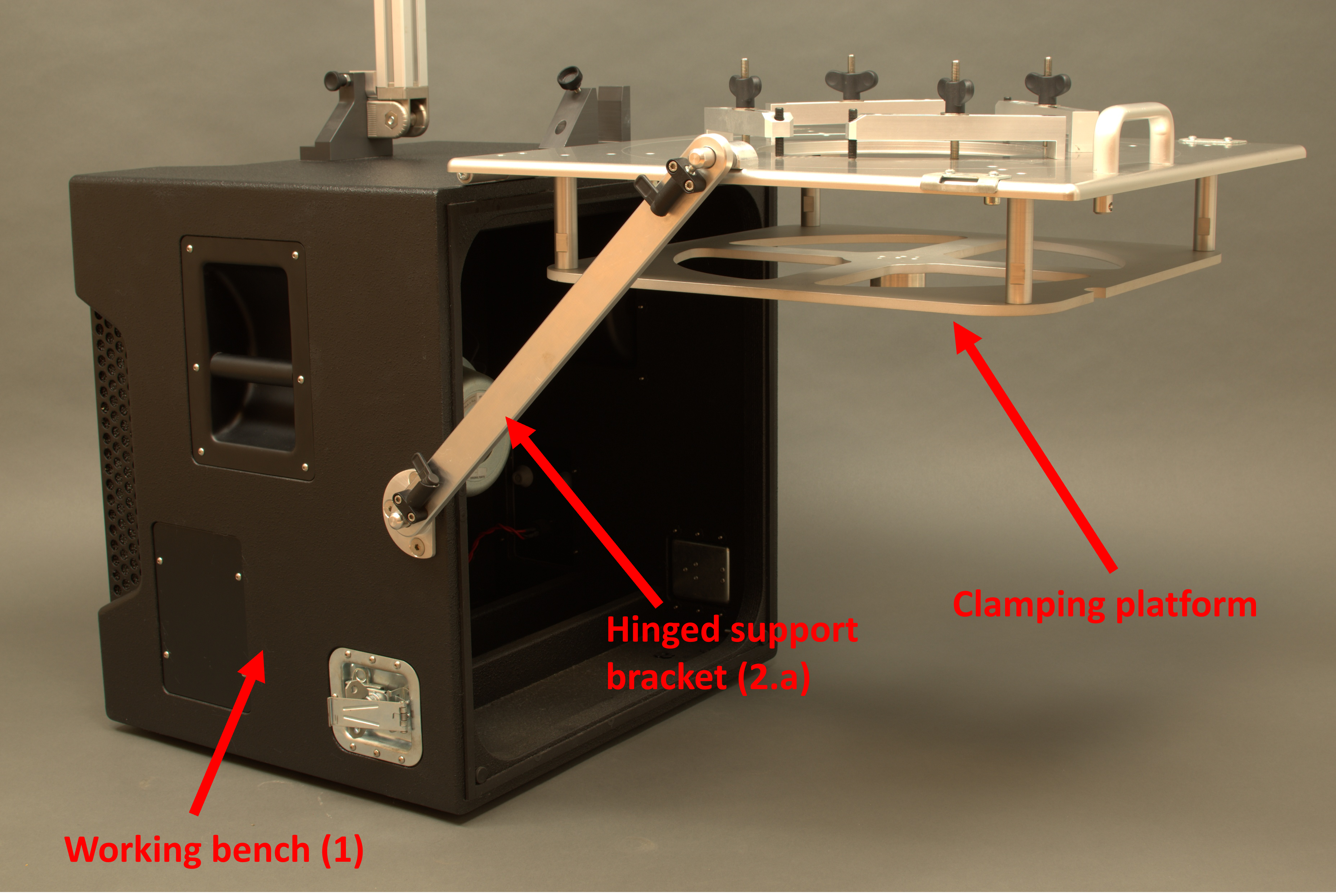
- 2.a Hinged support bracket - from revision 1.6
- Units: 1

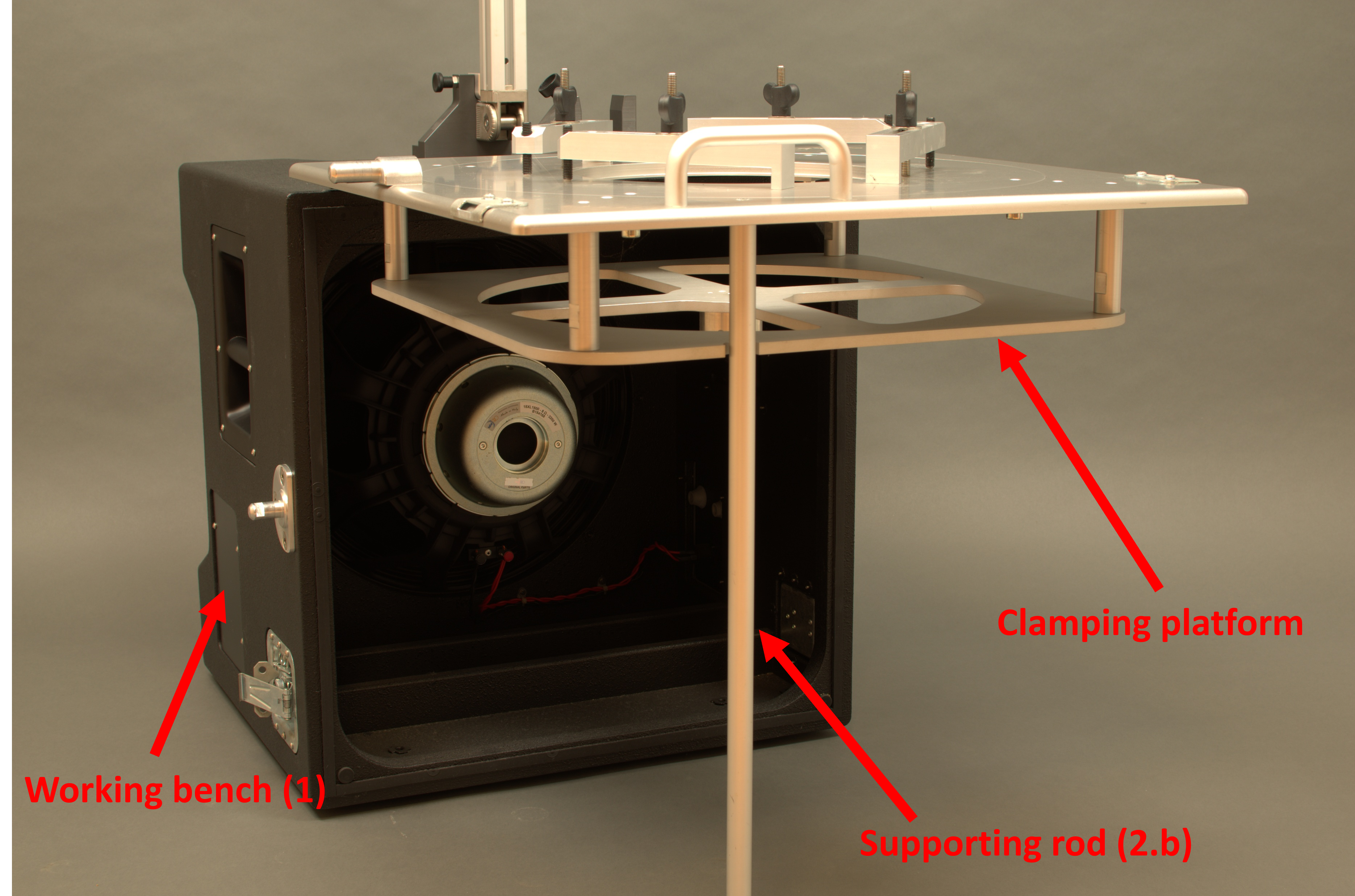
- 2.b Supporting rod (leg) - older than revision 1.6
- Units: 1

- 3 Guiding rod
- Units: 1Dimensions: 200 mmItem no.: 2500-152

- 4 Guiding rod
- Units: 1Dimensions: 315 mmItem no.: 1500-153
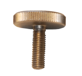
- 5 Hand screw
- Units: 1Dimensions: M6
for guiding rod
- 6 Sliding sleeve
- Units: 1Dimensions: 120 mmItem no.: 2600-154
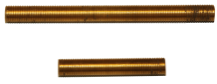
- 7 Sliding sleeve
- Units: 1Dimensions: 60 mmItem no.: 2600-155
- 8 Nuts for sleeve
- Units: 4Item no.: 2500-155
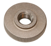
- 9 Calibration spacer
- Units: 1Item no.: 2201-004
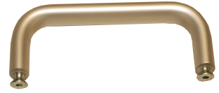
- 10 Handle for platform
- Units: 1
- 11 Countersunk screw for handle
- Units: 2Dimensions: M6x20
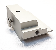
- 12 Laser rack
- Units: 1Item no.: 2600-140
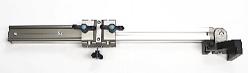
- 13 Mounting screw
- Units: 1Dimensions: M8x40
for the laser rack
- 14 Nut for mounting the laser rack
- Units: 1
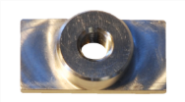
- 15 Fixture tool for sliding sleeve
- Units: 1Item no.: 2500-151
The screw can also be used to fix the calibration spacer.
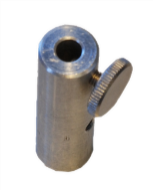
- 16 Laser clamping rest
- Units: 2
for holding rack horizontally
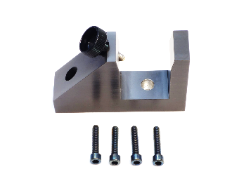
- 17 Allen screws for laser rest
- Units: 4Dimensions: M6x25 (30)
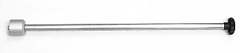
- 18 Laser rod
- Units: 1Item no.: 2211-009
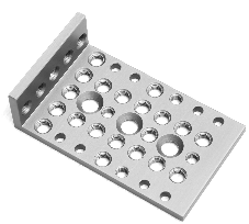
- 19 Laser bracket rev. 108
- Units: 1Item no.: 2211-016
- 20 Disc M4 for laser
- Units: 2
- 21 Allen screw for laser head
- Units: 2Dimensions: M4x25
- 22 Threaded bolt
- Units: 4Dimensions: M8x90
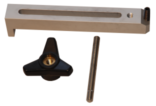
- 23 Clamping lever with thrust screw
- Units: 4Dimensions: M8x20
- 24 Turnbuckles
- Units: 4Dimensions: M8
- 25 Discs
- Units: 4Dimensions: M8 large
- 31 Cable speakON
- Units: 1Dimensions: 4 x 2.5 mm2, 5 m
- 50 Cable BNC
- Units: 1Dimensions: 5 m
- 51 Adapter BNC - SMB
- Units: 1

- 32 Tool for Allen screws
- Units: 1Dimensions: 2 mm
for laser
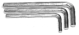
- 33 Tool for Allen screw
- Units: 1Dimensions: 4 mm
- 34 Tool for Allen screw
- Units: 1Dimensions: 5 mm
- 35 Tool for Allen screw
- Units: 1Dimensions: 6 mm
- 52 Plastic nut
- Units: 4Dimensions: M10x1
- 53 Washer
- Units: 4Dimensions: M8
high grade steel
- 54 Thrust screw
- Units: 4Dimensions: M8x20
with plastic head
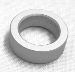
- 55 Spacer ring
- Units: 1Dimensions: Ø10 mm x 5 mm
aluminum
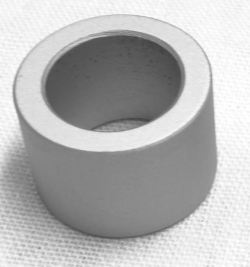
- 56 Spacer ring
- Units: 1Dimensions: Ø10 mm x 10 mm
aluminum
LST Bench#
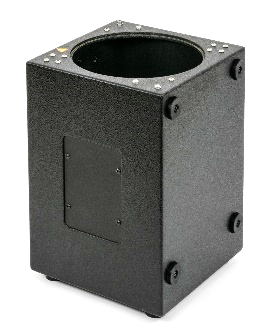
- 36 Work Bench
- Units: 1
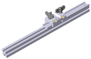
- 37 Laser rack
- Units: 1
- 38 Mounting screws
- Units: 2
for laser rack
- 39 Discs for screws (38)
- Units: 2
- 40 Laser rod
- Units: 1Item no.: 2211-009
- 41 Laser bracket rev. 108
- Units: 1Item no.: 2211-016
- 42 Disc M4
- Units: 2
for laser
- 43 Allen screw
- Units: 2Dimensions: M4x25
for laser head
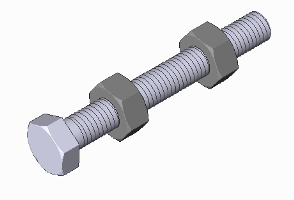
- 45 Reflective plastic hexagon bolt + knurled nuts
- (part of: Cone Set (plastic) for LST or SPM, item-no.: 2500-301)Bolt dimensions: M10x80Units: 2 bolts in rev.1.1, 3 bolts in rev.1.0Bolt dimensions: M10x40 | Units: 1 bolt in rev.1.1Nut dimensions: M10Units: 4 nuts
- 47 Cable speakON
- Units: 1Dimensions: 4 x 2.5 mm2, 5 m
- 48 Tool for Allen screw
- Units: 1Dimensions: 2 mm
for laser
- 49 Tool for Allen screw
- Units: 1Dimensions: 5 mm
for laser rack
Accessories#
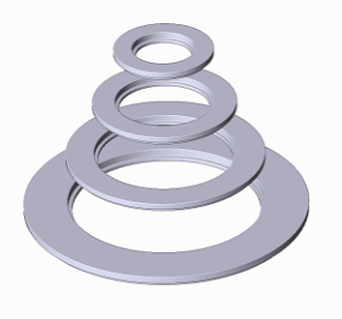
- 26 Ring set
- Units: 1
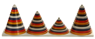
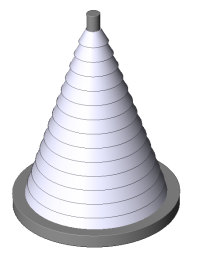
- 27 Cone set
- Units: 1
- 28 Cup set A
- Units: 1
- 29 Cup set B
- Units: 1
- 30 Cup set C
- Units: 1
- 44 Cone set
- Units: 1
light weight plastic
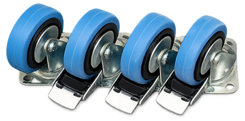
- 57 Wheels set
- Units: 1
Mounting Instructions (SPM Bench)#
Bring the clamping platform in horizontal position and lock it using the hinged support bracket (2.b).
For units prior to revision 1.6, rest the platform on the supporting rod (leg) (2.a) instead.
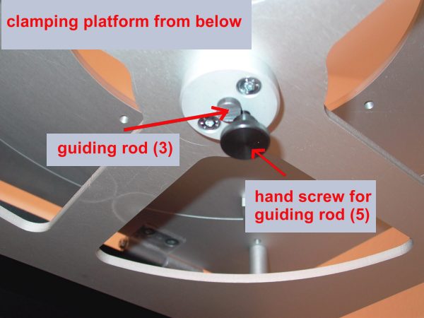
Insert guiding rod (3) into center hole of the clamping platform from below. Fasten guiding rod (3) at the rear side of the clamping platform by using the hand screw (5).
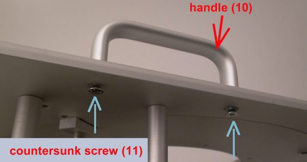
Fasten the handle for platform (10) by using the countersunk screw (11) M 6 x 20 mm.
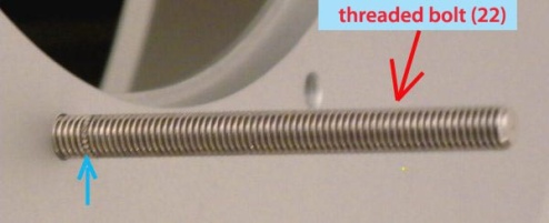
Insert threaded bolt (22) with 8 x 90 mm diameter into the clamping platform using the short side of the bolt with the 12mm thread width limited by ring. Screw all four threaded bolts (22) into the platform.
Put on the four levers (23).
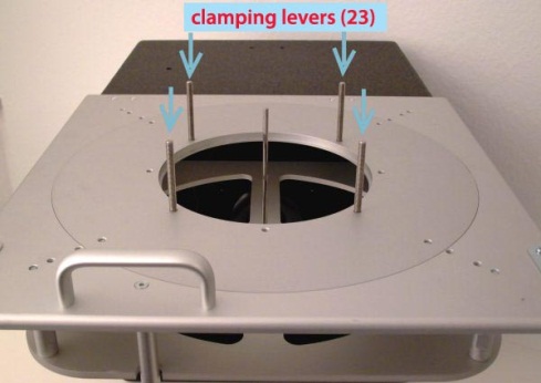
Fasten the levers (23) by using the M8 discs (25) …
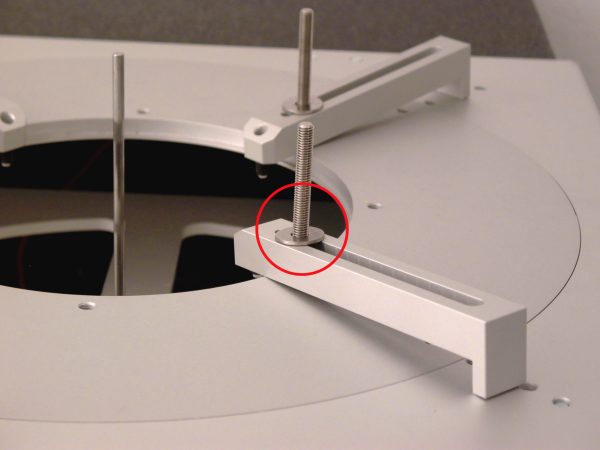
… and the turnbuckles (24)
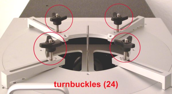
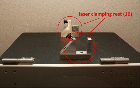
Fasten the two laser clamping rests (16) for horizontal position of the laser rack by using the four M6x25 Allen screws (17).
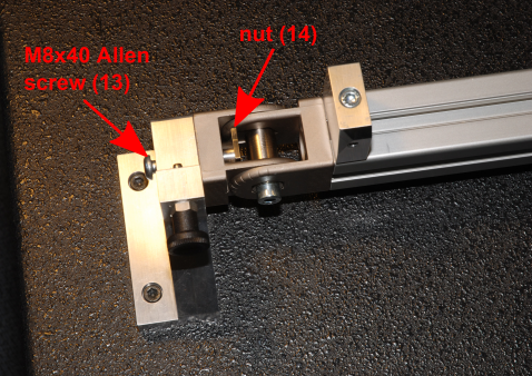
Put the laser rack (12) on the laser clamping rests (16). Fasten the rack by using the Allen screw (13) and nut (14).
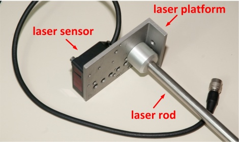
Screw the laser rod (18) into laser platform (19) and mount the laser head on the laser platform by using Allen screws M4x25 (21) and discs M4 (20).
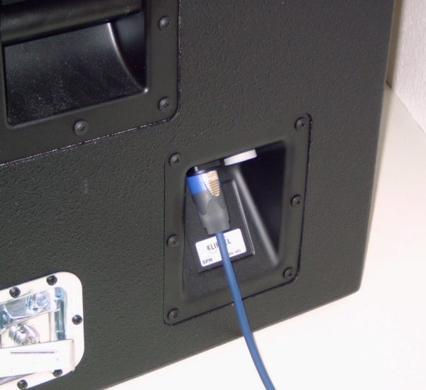
Connect the working bench (mounted loudspeaker) with the SPEAKER 1 or SP1 terminal at the analyzer device using the speakON cable. See KLIPPEL Analyzer Hardware for more details. Insert a microphone into the rubber terminal if you wish to perform linear parameter measurements (SPM Lite). To do so cut a small hole into the rubber plug that covers the microphone mounting plate. Two crossed cuts are favorable to fit with the microphone. If the microphone is not mounted (for SPM measurements) the hole can be closed with a microphone dummy (pencil) or with tape to avoid air noise.
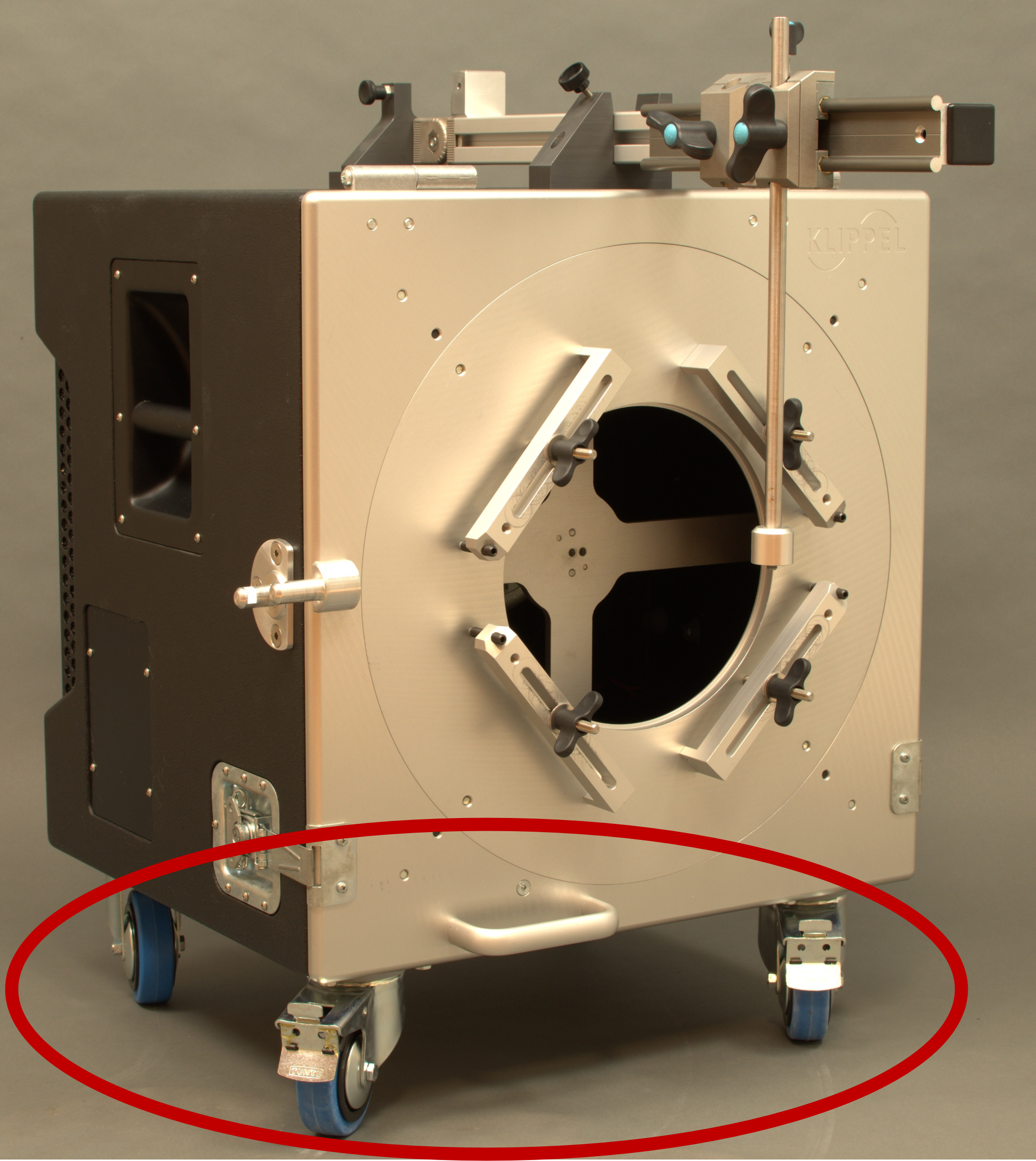
For revisions from 1.5 onward, wheels (57) can also be added, which improve the transportability of the SPM and make it easier to move; however, the wheels can be mounted at revision 1.5 on the driver side, and from revision 1.6 onward on both the driver side and the bottom side.
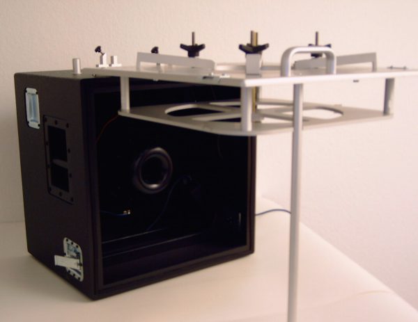
Find more information about clamping the suspension part in the SPM Tutorial.
Mounting Instructions (LST Bench Set – for External Laser Mounting)#
The extended LST bench provides an external boom for laser mounting. This allows more flexible adjustment of the laser and is therefore the preferred way of use for the SPM Lite.
Screw the laser rod into laser platform (19) and mount the laser head on the laser platform by using Allen screws M4x25 (21) and discs M4 (20).
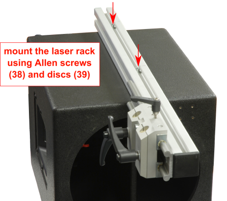
Mount the laser rack (37) to the test bench using Allen screws (38) and discs (39).
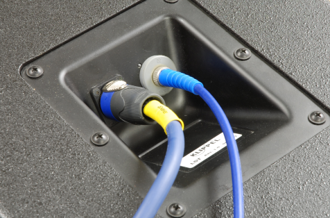
Connect the working bench (mounted loudspeaker) with the terminal SPEAKER 1 or SP1 at the analyzer device using the speakON cable. See KLIPPEL Analyzer Hardware for more details. Insert the microphone into the rubber terminal. To do so cut a small hole in the rubber plug that covers the microphone mounting plate. Two crossed cuts are favorable to fit with the microphone. If the microphone is not mounted (for SPM measurements) the hole can be closed with a microphone dummy (pencil) or with tape to avoid air noise.
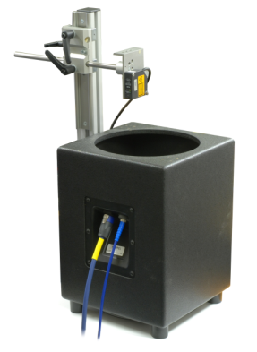
Attach the mounted laser platform to the laser rod (18) and attach it to the laser rack. Connect the laser head connection cable with the laser head using the female end of the cable (4 pin socket). Fix the connection using the provided screw ring.
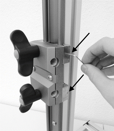
If the carriage is moving too easily or with too much force, you may adjust the friction of the carriage at the guide. Loosen or tighten the 1.5 mm hex socket screws using the 1.5 mm hex key according to your needs.
Setting up the System#
Note
The Suspension Part Measurement supports both Distortion Analyzer as well as Klippel Analyzer 3 hardware. For more information regarding the setup of your specific system, please refer to KLIPPEL Analyzer Hardware.
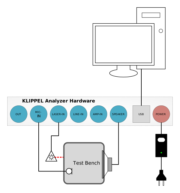
Connect the components in the following way:
The output OUT1 of the measurement device providing the stimulus signal is connected to the input of the power amplifier.
The output of the power amplifier is connected to the speakON connector AMP of the analyzer device.
The laser displacement sensor is connected to the laser input of the analyzer device.
The microphone is connected to the microphone input of the analyzer.
Note
This is only needed for the small signal measurements (SPM Lite).
The output SPEAKER 1 or SP1 of the analyzer device is connected to the working bench by using the special SPM speaker cable.
SPM Tutorial#
What is the Goal of This Tutorial?#
The Tutorial gives step-by-step instructions on how to use the suspension part measurement (SPM).
The first part – Tutorial 1 – Viewing the Results of the Nonlinear Stiffness Measurement (SPM Pro only) interprets the results of the SPM Pro.
The second part – Tutorial 2 – Performing a Measurement of the Nonlinear Stiffness K(x) (SPM Pro only) – describes how to measure the large signal behavior of your own suspension part.
The third part – Tutorial 3 – Customizing SPM Pro provides tips how to get the most out of SPM.
The fourth part – Tutorial 4 – Performing a Measurement of the Linear Stiffness – describes how to measure the stiffness and other parameters in the small signal domain.
Tutorial 1 – Viewing the Results of the Nonlinear Stiffness Measurement (SPM Pro only)#
Example data used in this manual is stored in the Web Example database. If not downloaded already, get it from the latest R&D release <https://www.klippel.de/go/current-rnd-release> and open the web-based database.
See also
View Results for general information on how to download this database, open and view results in dB-Lab.
Open the object Transducer Part + Material (SPM, MSPM, LST, BFS, MPM) - SPM Suspension Part. For information on how to navigate within dB-Lab please read the dB-Lab – Software manual.
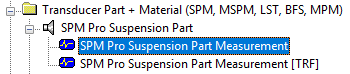
Open the result window K(x) Stiffness by performing a double click on the operation SPM Pro Suspension Part Measurement.
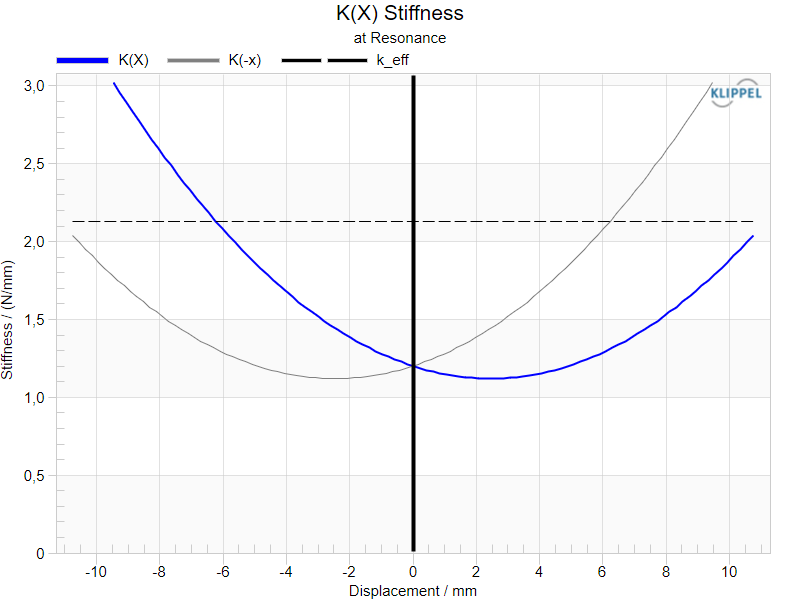
The dashed curve shows the effective stiffness \(k_{\mathrm{eff}}\) of the suspension in the working range (\(-9 \: \mathrm{mm} < x < 11 \: \mathrm{mm}\)). The blue solid curve shows the stiffness \(K(x)\) versus displacement \(x\).
Nonlinear Stiffness K(x)#
In contrast to the linear model the stiffness of a real suspension is not constant but varies with displacement \(x\). Thus, the stiffness \(K(x)\) versus displacement reveals the nonlinearity of the suspension part. The \(K(x)\) shown in the previous diagram shows that the stiffness at negative displacement \(x = -9 \:\mathrm{mm}\) is approximately 3 times higher than at the rest position \(x = 0\). There is also a distinct asymmetry in the curve. The stiffness at positive displacement \(x = +11 \:\mathrm{mm}\) is only about 60 % of the stiffness at negative displacement \(x = -9 \:\mathrm{mm}\). Under dynamic operation an AC‑signal is partially rectified and a positive DC-component of 3 mm is generated.
Effective Stiffness keff#
The effective stiffness \(k_{\mathrm{eff}}\) neglects any variation of the stiffness versus displacement but represents the effective behavior by a single value which depends on the signal properties of the stimulus and the peak displacement occurred during measurement. In the large signal domain, the effective stiffness usually increases with amplitude which is caused by the nonlinearity of the suspension. In the small signal domain, the effective stiffness may decrease with rising amplitude which is caused by visco-elastic effects of the suspension material. To ensure comparability of the results it is strongly recommended to state the peak displacement \(X_{\mathrm{peak}}\) for which the effective stiffness \(k_{\mathrm{eff}}(X_{\mathrm{peak}})\) is valid such as
This value is simple to interpret and corresponds directly to the resonance frequency \(f_{\mathrm{r}}\) and the moving mass \(m\). The single-number representation of \(K(x)\) may be sufficient and convenient for QC applications.
Nonlinear Compliance C(x)#
Open the window C(x) Compliance by doubling clicking on the corresponding entry in the results windows list in dB-Lab.
See also
The dB-Lab manual describes how to customize results windows and curves.
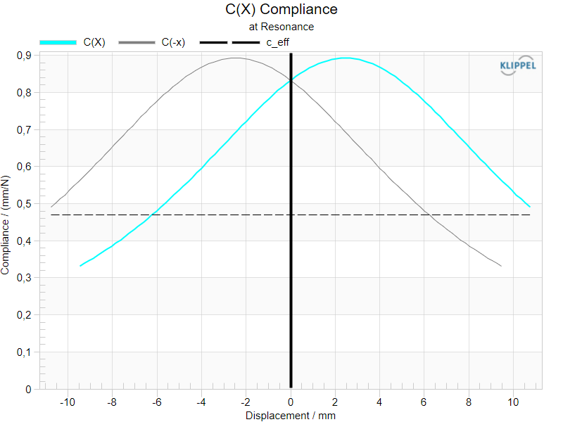
The compliance \(C(x)\) is the inverse of the stiffness \(K(x)\). It shows a bell-shaped curve which corresponds to the parabolic shape found in the \(K(x)\) characteristic. However, the stiffness curve reveals details of the nonlinearity clearer than the compliance curve and is more recommended for graphical representation.
Tutorial 2 – Performing a Measurement of the Nonlinear Stiffness K(x) (SPM Pro only)#
Measurement procedure:
Clamping the DUT
Setting up measurement properties
Performing an automatic measurement
Clamping the DUT#
The clamping of the suspension part is done as described in chapter SPM Bench. You may also watch the demo video on the SPM module website. Do not forget to weigh the suspension part including the inner clamping before mounting.
Warning
Ensure that the DUT is clamped firmly. Loose parts can damage the laser sensor or cause injuries!
Setting Up Measurement Properties#
Start dB-Lab and create a new object using the operation template SPM Pro Single Measurement (Spiders and Cones). Open the Property Page Setup and enter the following information into the property page:
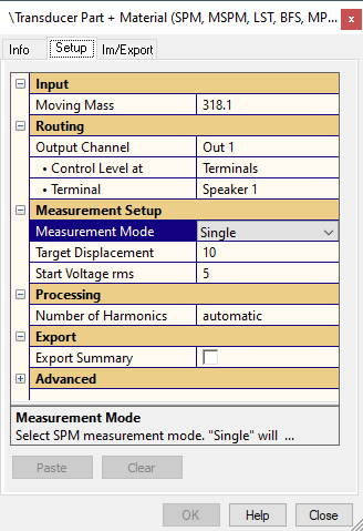
- Mass
Enter the moving mass (suspension + inner clamping part) in grams.
- Target Displacement
Enter the peak displacement, which should be used as a target value.
- Start Voltage
Adjust the start voltage if necessary.
Note
Too small values will increase the measurement time. Too large values may cause the displacement to exceed the target value significantly and damage the DUT.
- Number of Harmonics
Select the order of harmonics for the power series fitting of the nonlinear stiffness:
automatic (automatically determines number of harmonics)
3 (normally applicable for spider)
5 (normally applicable for surround)
Performing the Measurement#
Press the Run button  to start the measurement. A series of pre-measurements
will be performed running in a loop to automatically adjust the stimulus (voltage and frequency range of the sweep).
The instantaneous voltage and the resulting displacement will be displayed during
the measurement. The running measurement can be canceled at any time by pressing
the Cancel button
to start the measurement. A series of pre-measurements
will be performed running in a loop to automatically adjust the stimulus (voltage and frequency range of the sweep).
The instantaneous voltage and the resulting displacement will be displayed during
the measurement. The running measurement can be canceled at any time by pressing
the Cancel button  . If the target displacement cannot be accomplished
within 10 measurements, the measurement will be finished and a warning will be generated.
. If the target displacement cannot be accomplished
within 10 measurements, the measurement will be finished and a warning will be generated.
Note
The start-up voltage of the measurement might be too high for some DUTs with lower stiffness. If the current displacement exceeds the desired target displacement significantly then stop the measurement and restart it with a reduced Start Voltage. To reduce the measurement time, it might be helpful to increase the Start Voltage.
Tutorial 3 – Customizing SPM Pro#
Suspension parts are usually made out of material such as impregnated cloth, paper, foam, rubber with properties changing over time. There is a dependency on the ambient conditions (temperature, humidity) and some memory effects related to the way the suspension parts are manufactured and stored. Besides that, there are also reversible and non-reversible processes in the suspension itself which have very short and very long-time constants.
The third part of the tutorial gives some tips for the advanced user to consider the influence of the following factors:
way of clamping the suspension part
additional mass of the inner clamping parts
influence of the stimulus
maximal order \(N\) of the power series expansion used for \(K(x)\)
uncontrolled variables
reversible and irreversible changes in the suspension material
Repeatability and Reproducibility#
The repeatability of the measurement technique has been tested on suspension parts without changing the clamping and the setup. The results are very reproducible (< 1 %). Repeating the measurement more than 10 times shows a systematic decrease of the stiffness at \(x = 0\) to lower values. This effect can be reduced by exposing test objects to a break-in procedure (5 min vibration at resonance) before the measurements. This effect is closely related to the ageing of the suspension.
Way of Clamping#
The outer clamping has a minor influence on the measurement results. Even operation faults such as using rings which are too small or are not applied concentrically cause relatively small errors.
The inner clamping is much more critical. Some care is required to ensure that the friction of the slide on the rod is small, so that the displacement of the inner corrugation roles is not limited by the inner clamping parts. The center of gravity and the outer clamping plane should be approximately in the middle of the slide. If the friction is too high giving a low \(Q\) of the resonator, then the maximum of the transfer function \(H_{\mathrm{x}}(\mathrm{j}\omega)\) occurs below resonance frequency giving a smaller estimate of the stiffness.
Note
Systematic differences may occur between measurements performed with a suspension glued to loudspeaker parts and the same suspension clamped by universal set of parts. However, these differences are reproducible and should be considered in the design process. The non-destructive testing (using a universal clamping system) is advantageous for the quality control of the suspension parts.
Order of the Harmonics#
The nonlinearities of the stiffness \(K(x)\) and compliance \(C(x)\) are calculated from the harmonics detected in the displacement signal. Unfortunately, the laser signal is affected by noise and artifacts will be produced in the measured curve if noisy harmonics are considered.
There are two options to exclude noisy harmonics:
The setting Number of Harmonics on the property page is set to automatic. The number of valid harmonics is measured automatically and displayed in the window Table Setup and Result Parameters.
The setting Number of Harmonics is set manually to three or five. For the spider a value of three should be sufficient and for cone-surround-assemblies or passive radiators a value of five is recommended.
Note
The order of the harmonics will change the shape of the nonlinear curve. If three harmonics are used, the nonlinear curve will have an order of two and thus only a parabola is used. If the order is too high, noise can corrupt the measurement results.
Mass of the Inner Clamping Parts#
The influence of the mass added to the inner clamping part is relatively small. However, using very large clamping parts (more than required to clamp the suspension) will lower the resulting resonance frequency. Assuming a constant resistance (friction of the slide on the guiding rod and internal losses of the suspension part), this resonance frequency reduction causes an increasing Q-factor, giving a much more distinct resonance peak.
However, the measurements of spiders at very low frequencies usually lead to a smaller measured stiffness than at higher frequencies due to viscoelastic effects (creep) of the suspension. The creep factor as measured in the LPM – Linear Parameter Measurement describes the variation of the stiffness (compliance) versus frequency in the small signal domain.
Friction of the Guiding Rod#
The friction of the sliding sleeve on the guiding rod and the internal losses in the suspension material have no influence on the measured stiffness as long as the loss factor is sufficiently high (\(Q > 2\)) and the resonance frequency can be detected by a distinct peak in the transfer function (displacement divided by voltage or displacement divided by sound pressure inside the box). In case a warning message is displayed, the clamping of the suspension part should be checked.
Amplitude of the Stimulus#
Due to viscoelastic mechanisms in the suspension material, the measured stiffness characteristic depends on the amplitude of the signal.
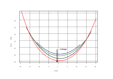
The figure above shows the nonlinear stiffness characteristic measured with different stimulus voltages. While the curves at positive and negative peak values \(x_{\mathrm{peak}}\) almost coincide, there is a significant decrease of stiffness \(K(x=0)\) at the rest position \(x=0\). This is an irregular behavior of the suspension material (cloth, rubber, and impregnation) and not an artifact caused by the measurement technique. The loss of stiffness at \(x=0\) is almost reversible and original properties will be restored after a few seconds. Non-reversible changes caused by ageing and initial usage (breaking-in) are discussed below. The same behavior has also been observed in finally assembled loudspeakers using other static, incremental dynamic or full dynamic methods.
A simple explanation for this phenomenon is that a stretching of the corrugation roles at high amplitudes causes a temporary deformation of the fiber structure and makes the suspension softer between the positive and negative peak values. However, this kind of deformation is reversible and the time constant is relatively short. It stays only for multiple periods of the ac signal and recovers completely after a few seconds. This effect depends on the geometry and impregnation of the suspension material. It increases the nonlinearity of the suspension which becomes not only stiffer for larger displacement but also softer between the excursion maxima.
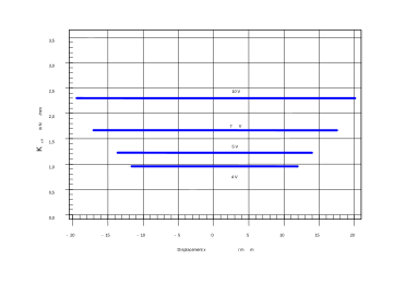
The effective stiffness \(K_{\mathrm{eff}}(x_{\mathrm{peak}})\) depends on the maximal peak displacement \(x_{\mathrm{peak}}\) occurred during measurement. The figure above shows the variation of the effective stiffness of a 3-inch spider measured with iteratively increased voltages from 4 to 10 V at the terminals of the loudspeaker. The substantial variations at higher amplitudes are mainly caused by the nonlinear increase of the stiffness at higher displacements. At small signal amplitudes, the visco-elastic effect may dominate the increase of the stiffness at the positive and negative peak values. Thus, the effective stiffness \(K_{\mathrm{eff}}(x_{\mathrm{peak}})\) and resonance frequency \(\omega_{\mathrm{r}}(x_{\mathrm{peak}})\) may fall with rising peak displacement.
Influence of Test Time#
The dynamic measurement technique is also convenient for the investigation of the break-in and other ageing effects of the suspension. The figure below shows the change of the stiffness versus time. While performing a permanent excitation of the spider with a sweep, the stiffness was measured in intervals of 15 minutes.
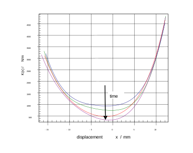
Variation of the nonlinear stiffness \(K(x)\) during long term testing of a spider (measured in 15 min intervals)
It is interesting to see that the stiffness at higher displacements stays constant but the stiffness at the rest position \(x = 0\) is reduced to 30 %. Thus, the stiffness at high positive and negative displacements is closely related to the geometry of the suspension, while the stiffness at rest position is mainly determined by the impregnation and thickness of the material.
Tutorial 4 – Performing a Measurement of the Linear Stiffness#
Measurement procedure:
Clamping the DUT
Setting up the stimulus
Performing a TRF
Adding mass to the DUT
Performing another TRF
Select the measured TRF operations in the SPM Lite setup
Running the SPM Lite
Clamping the DUT#
SPM Bench#
The clamping of the suspension part is done as described in chapter SPM Bench. To reduce damping, remove the guiding rod.
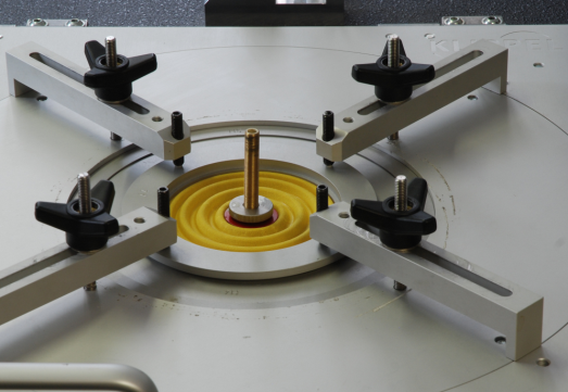
Shut the test bench. Direct the laser beam to the inner clamping part. It is recommended to calibrate the laser to judge the peak displacement during the measurement. Absolute calibration is not required for determining the linear parameters, however. Make sure that the laser is in its center position. 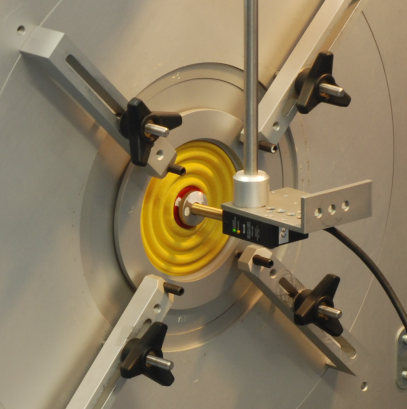
LST Bench#
For clamping instructions refer to the SPM Reference (see chapter LST Bench).
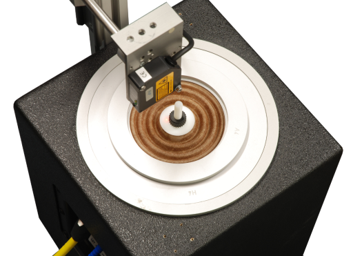
Direct the laser beam to the inner mounting part (cone). Adjust the laser position so that the laser is in its center position.
Setting Up the Stimulus#
The aim of this section is to explain how to set up a suitable stimulus. The target is driving the DUT in the small signal domain while having a sufficient signal-to-noise ratio in displacement laser signal.
Start dB-Lab and create a new object using the object template SPM Lite Added Mass Method. Run the object 1 TRF Setup with the default settings.
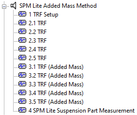
Double-click on the object 1 TRF Setup to see the transfer function \(H(f)\) between sound pressure and displacement as well as the spectra of the microphone and laser signals. By looking at the \(H(f)\) curve it should be possible to spot the resonance peak caused by the suspension part. It is recommended to keep the suspension part displacement below 1 mm for proper small signal measurement. Please check window y2(t) Input Waveform for peak displacement in the laser signal. If the displacement was too high, decrease the stimulus voltage and repeat the measurement.
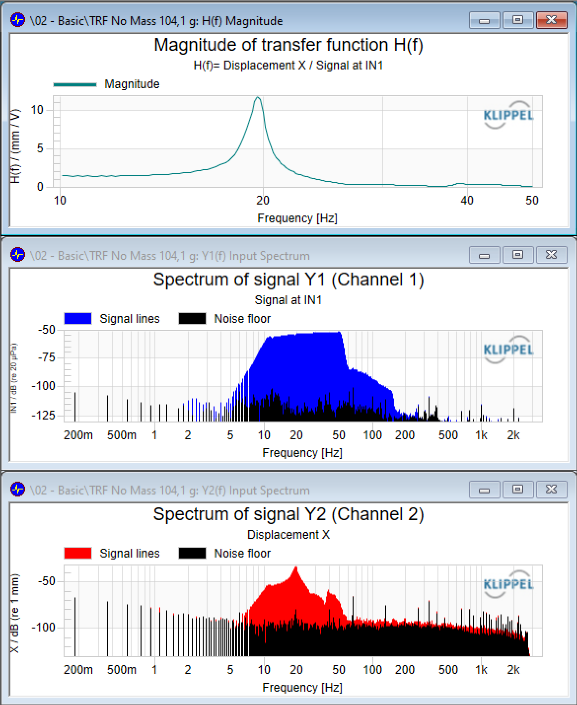
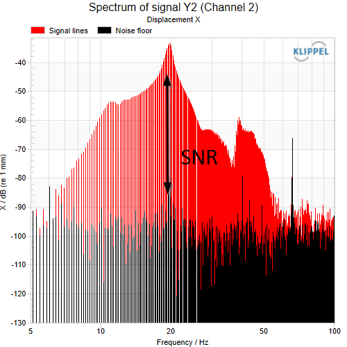
- By looking to the spectrum of the laser signal (Y2(f) Input Spectrum), make sure that the signal-to-noise ratio is at least 25 dB at the resonance frequency.
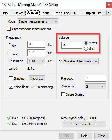
If the signal is dominated by noise, increase the stimulus voltage in the Input tab of the Property Page of the TRF operation and repeat the measurement.
In case the highest magnitude of the \(H(f)\) curve does not occur at the resonance frequency, limit the frequency range to e.g.: \(f_{\mathrm{max}} = 2.5\) times the resonance frequency. This may also be useful to minimize measurement time. Once you have found a suitable stimulus voltage, copy the stimulus settings to the operations 2.1 TRF No Mass and 3.1 TRF (Added Mass) using the Im/Export tab of the TRF.
Performing a TRF#
Run the operation 2.1 TRF.
Adding a Mass#
Now add a defined mass to the suspension part to shift the resonance frequency. If using the SPM bench, you may screw one or multiple metal nuts (8) on the sliding sleeve.
If using the LST bench with unmodified clamping you may add a cone from the LST cone set (44) to the inner clamping. This has the advantage that you do not need a scale because the weights of the cones are written in a table (see Ring Set for Inner Clamping (LST Bench)). Do not forget to adjust the laser to its center position.
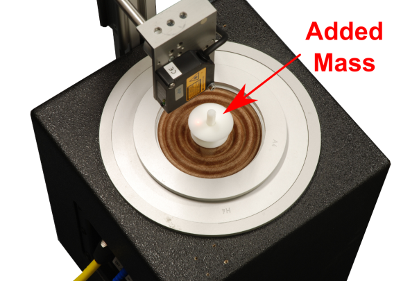
The mass should have a weight of around 50 % to 100 % of the suspension part including the inner clamping parts.
Performing a TRF with Added Mass#
Run the operation 3.1 TRF (Added Mass).
Performing Additional TRF Measurements#
The measured sample may tilt during the TRF measurement, for instance due to a mass imbalance caused by the inner clamping parts. To improve the measurement results, up to five TRF measurements with and without mass can be processed by the SPM Lite. The results will be calculated and averaged. When the TRF measurements are performed in various positions at and around the center of the inner clamping parts, the spatial averaging will reduce the influence of a tilting movement of the sample.
Importing the TRF Results to the SPM Lite Operation#
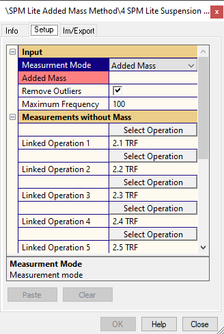
Open the Property Page of the SPM Lite operation. Enter the value of the added mass (in gram) in the input field of the parameter Added Mass. Check that the names specified by the parameters Linked Operation 1-5 show the names of the TRF operations that are to be used for the SPM Lite. They should already be correct if the names of the TRF operations of the template have not been altered.
Note
If a linked operation has not been measured and therefore has no valid result data, the SPM Lite will ignore the operation. In this case, an information message will be displayed at the top of the Table Results window.
Calculation of the Results#
Run  the operation 4 SPM Lite Suspension Part Measurement. In case of errors or
warnings refer to the section Overview of the chapter Malfunction and Troubleshooting. When
double-clicking on 4 SPM Lite Suspension Part Measurement you see the results of the SPM Lite operation computing the linear parameters.
the operation 4 SPM Lite Suspension Part Measurement. In case of errors or
warnings refer to the section Overview of the chapter Malfunction and Troubleshooting. When
double-clicking on 4 SPM Lite Suspension Part Measurement you see the results of the SPM Lite operation computing the linear parameters.
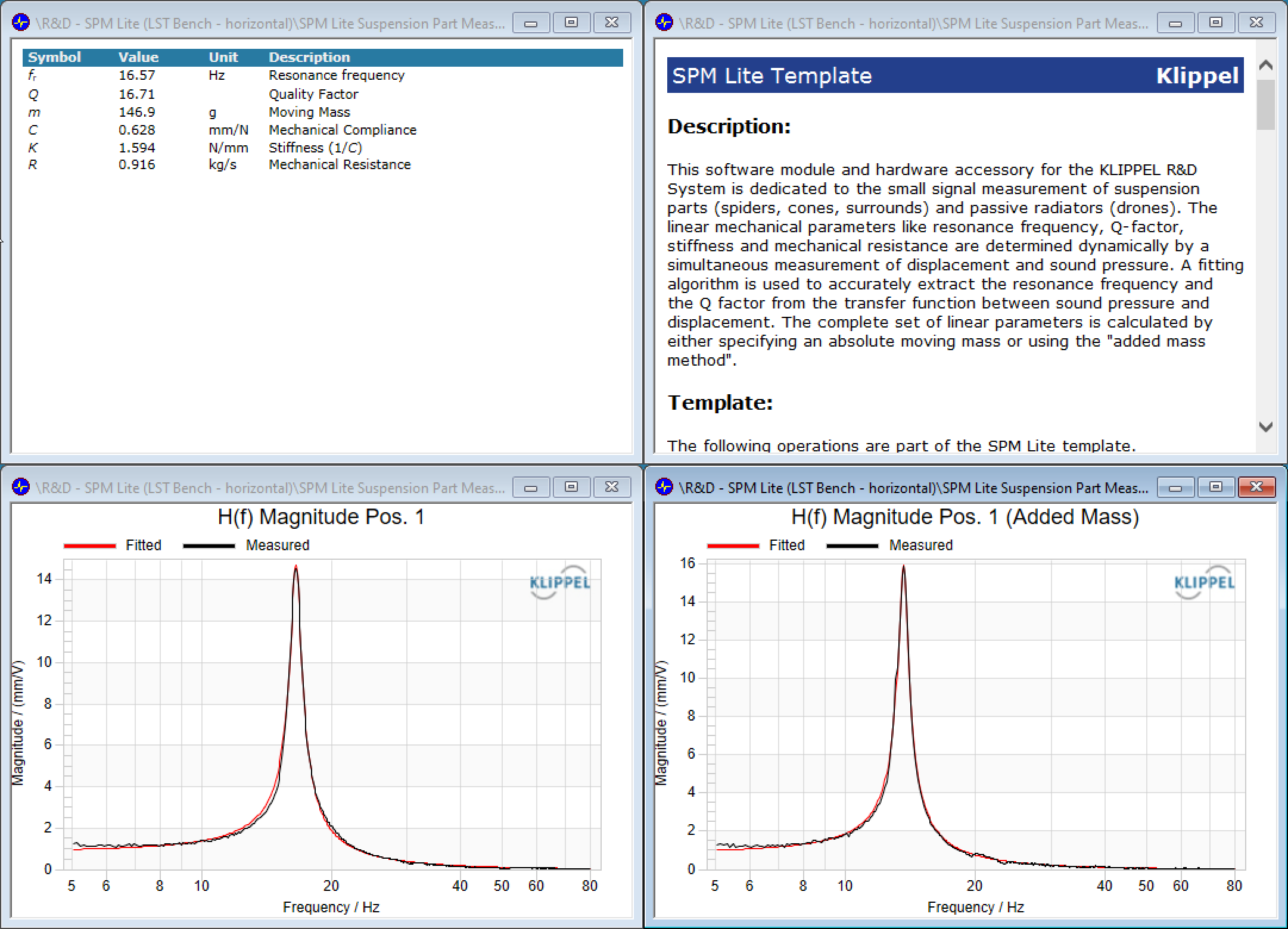
In the upper right window Table Results, the identified parameters can be inspected. Also warning and error messages will appear in this window as well as in the Protocol window.
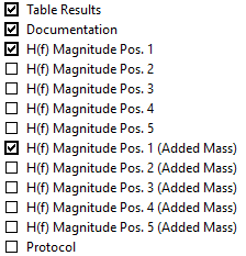
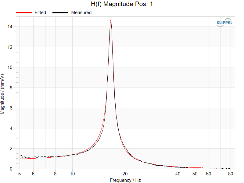
To verify the validity of the calculated parameters it is advised to compare the measured curves with the fitted curves (H(f) Magnitude Pos. 1 … 5 …). If measured and fitted curves match well in frequency band around the resonance peak, the derived parameters were determined correctly.
SPM Reference#
Clamping#
Note
The way of clamping the suspension part affects the final performance. Consistent clamping is important for consistent results.
SPM Bench#
Warning
Make sure both the inner and outer clamping are firm enough to withstand the forces during operation at maximum drive voltage! Use a sensible maximum voltage setting! If the clamping detaches during operation, moving parts may damage the laser sensor or other hardware.
Procedure
Selection of inner clamping parts
Inner clamping
Selection of outer clamping parts
Outer clamping
During the dynamic testing the suspension part should be clamped in a similar way as mounted in the final loudspeaker. In some cases, it may be convenient to use adhesive and original loudspeaker parts (voice coil former, frame) for clamping. However, nondestructive testing is preferred for comparing samples, storing reference units and for simplifying the communication between manufacturer and customer.
Selection of Inner Clamping Parts#
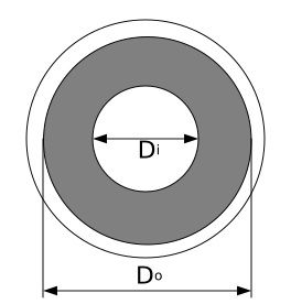
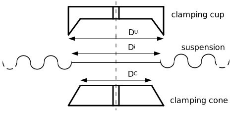
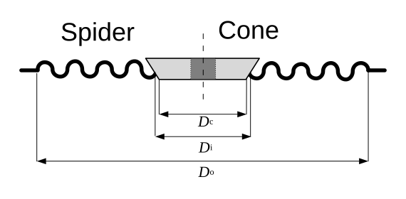
\(D_{\mathrm{i}}\) is the inner diameter at the neck of the suspension part.
\(D_{\mathrm{o}}\) is the outer diameter of the suspension part without rim.
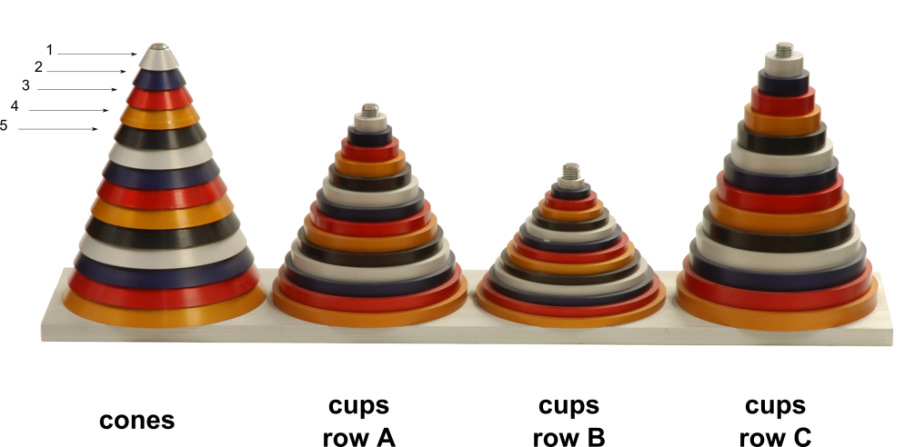
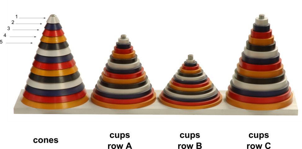
Select the cone that fits the part to be measured. See the (section Ring Set for Inner Clamping (SPM Bench)) for dimensions of cones and cups or slide the suspension on the cone stack to find the optimal cone part.
The inner diameter \(D_{\mathrm{i}}\) of the suspension has to be larger than the cone diameter \(D_{\mathrm{C}}\) and smaller than the cup diameter \(D_{\mathrm{U}}\). For each cone there are three different cups with different diameters \(D_{\mathrm{U}}\) provided which are marked by the same color code. This allows a firm clamping of the neck of the suspension at the outermost rim at an angle of about 50 degree.
For example: The spider has a \(D_{\mathrm{i}}\) of 65 mm. Choose the red cone number 8 with 60 mm and the red cup which fits best: C8.
Inner Clamping of the Suspension#
Spider
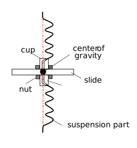
Cone
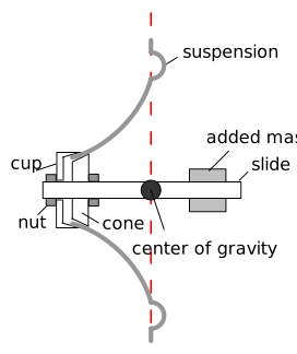
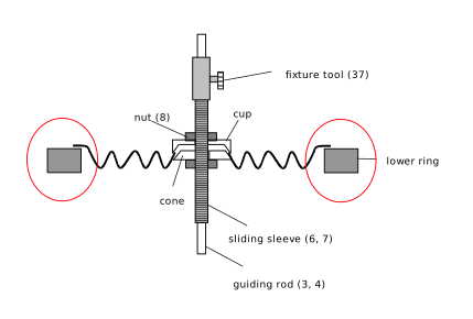
The neck of the suspension is clamped between cone and cup on a slide sleeve (6 or 7) by using two nuts (8). The slide is a small sleeve equipped with a special bearing made of Teflon reducing the friction on the guiding rod (3 or 4) (polished and coated with titanium). The suspension has to be clamped on the slide in such a way that the outer rim of the suspension is in the middle of the slide. The center of gravity has to be in the middle of the slide. This reduces tilting of the suspension, irregular vibration and ensures minimal friction at the rod. For very asymmetric suspension parts an additional mass (use some of the additional nuts (8) provided) may be added on the other side.
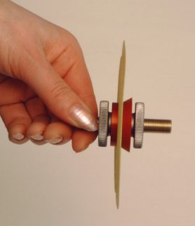
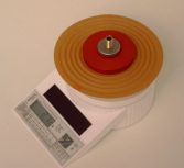
Measure the weight of the suspension with inner clamping parts. It will be needed by the post processing software later.
Selection of Clamping Rings for Outer Clamping#
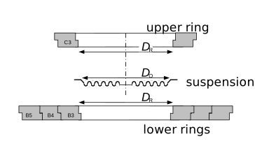
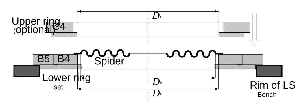
- Select the outer rings: The outer diameter \(D_{\mathrm{o}}\) of the suspension part should be just smaller than the ring diameter \(D_{\mathrm{R}}\) (see look-up table below).For example: The spider has a \(D_{\mathrm{o}}\) of 87 mm. The look-up table below shows that B3 with \(D_{\mathrm{R}}= 89 \:\mathrm{mm}\) is just greater than \(D_{\mathrm{o}}\).
- The lower ring set is completed by selecting all rings which have the same character in the nomenclature and are larger than the outer clamping ring.For example: Select B5-B4-B3.
- The next larger ring is used as upper clamping ring because this ring has a rim on the opposite site with the same diameter \(D_{\mathrm{R}}\) as the lower clamping ring.For example: Select ring C3 which follows ring B3 in the table Ring Set for Outer Clamping.
Outer Clamping of the Suspension#
Put the laser rack with laser in vertical position. Open the workbench and bring the clamping platform in horizontal position, by using the hinged support bracket (2.a) or supporting rod (leg) (2.b), depending on your revision. If the suspension will be measured at high amplitudes with more than 2 mm, then use the guiding rod to ensure a one-dimensional movement of the suspension. Consequently, remove the guiding rod if the measurement will be performed at low amplitudes to avoid additional friction (stiction).
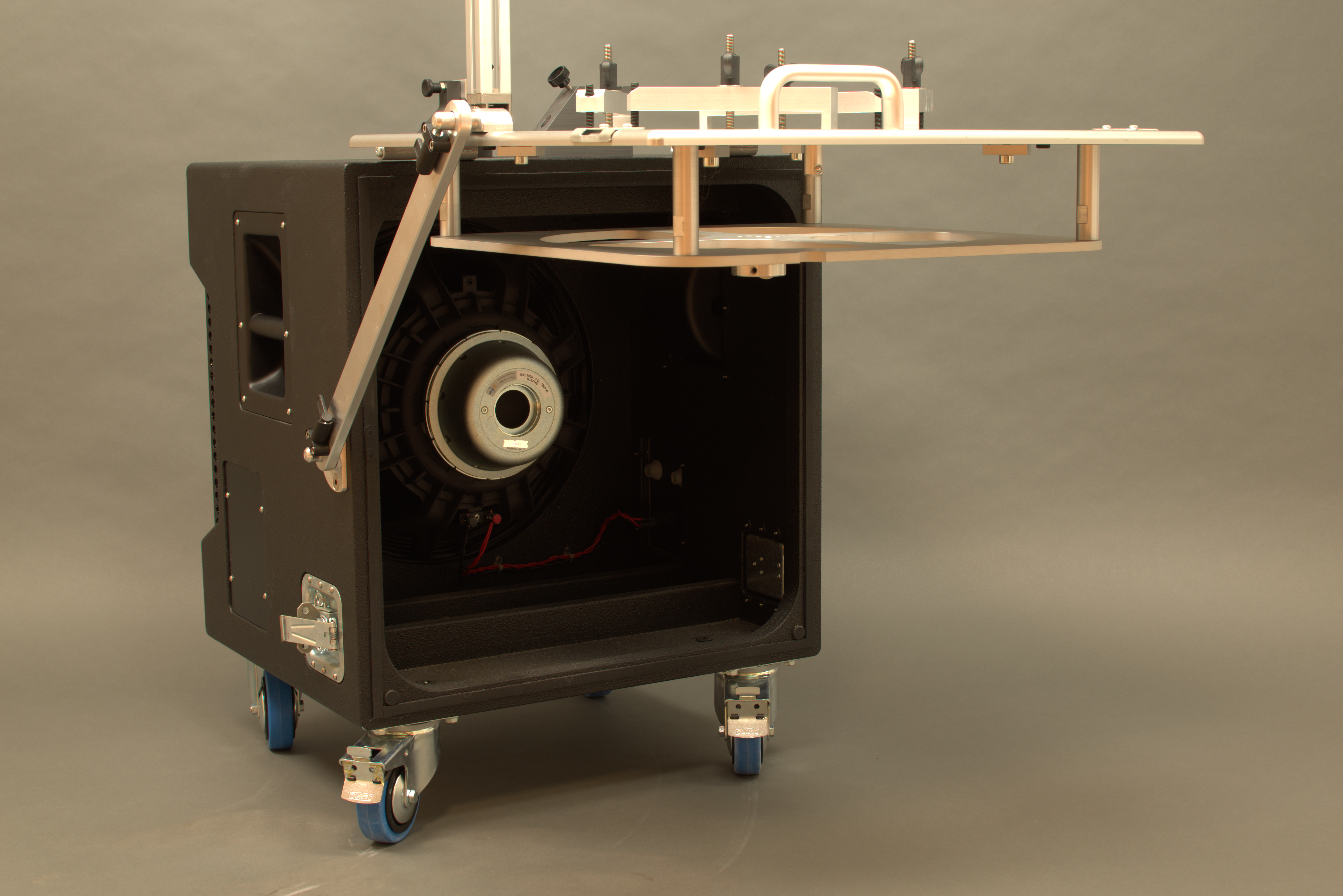
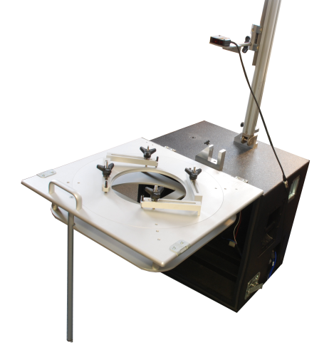
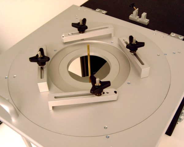
Put the lower clamping rings into the platform.
Example: Start with the largest ring C5 followed by C4.
Screw the fixture tool (15) on the sliding sleeve (6 or 7). Loosen the hand screw on the fixture tool.
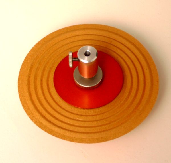
Put the slide with the clamped suspension on the guiding rod (if used). Adjust the position of the inner clamping part on the guiding rod in such a way that the outer rim of the spider just touches the lower ring. Fasten the hand screw on the fixture tool. If no guiding rod is used center the suspension part carefully on the lower clamping ring.
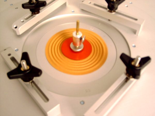
Put the upper clamping ring on the suspension. Put the clamping levers on the upper clamping ring and fasten the four turnbuckles simultaneously (in a diagonal order). The clamping levers should be in a horizontal position approximately. The thrust screws on the levers may be adjusted by using an Allen tool. Remove the fixture tool from the rod or fasten the fixture on the rod at sufficient distance from the slide and check that the clamped suspension part may slide smoothly on the rod.
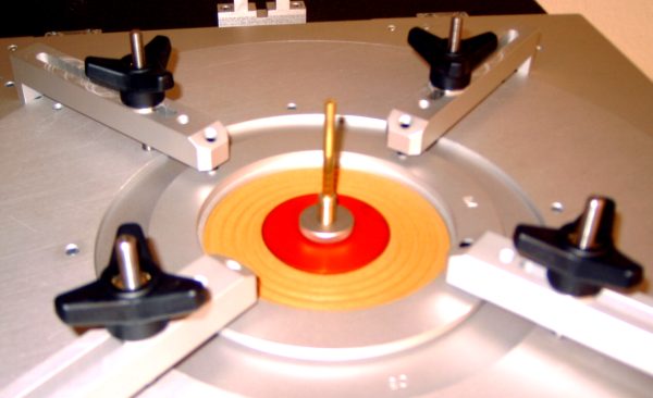
Depending on the revision, remove the hinged support bracket (2.a) or supporting rod (leg) (2.b) and close the box. Bring the laser rack in horizontal position and fasten the hand screw on the front laser rest firmly. For laser calibration, please refer to KLIPPEL Analyzer Hardware manual chapter Calibration and Verification.
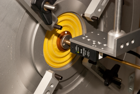
Adjust the laser beam to the inner clamping part. Ensure that the displacement laser is at center position (ANR laser type: yellow and green light must be on. The yellow light stops flashing). Put a dot of white ink on the inner clamping part to increase the reflected light and to ensure sufficient signal to noise ratio.
LST Bench#
Procedure
Inner Clamping
Outer Clamping
Note
In this section it is described how to clamp suspension parts to the original LST bench as delivered by KLIPPEL. Both horizontal and vertical mounting is possible (using fast clampers or a custom mounting platform): Horizontal clamping may not be optimal in some cases due to static displacement caused by mass of the inner clamping parts. This may change the working point on the nonlinear stiffness curve \(K(x)\). Especially for the added mass method, this can lead to inaccuracies as the stiffness is not constant among the measurements with and without added mass. Therefore, it is recommended to measure suspension parts in a vertical orientation. In case horizontal mounting is preferred, the user has the opportunity to determine the moving mass using a high precision scale instead of the added mass method. This is especially beneficial if large and soft suspension parts shall be measured.
Inner Clamping#
\(D_{\mathrm{i}}\) is the inner diameter at the neck of the suspension part. \(D_{\mathrm{o}}\) is the outer diameter of the suspension part without rim.
Select the cone that fits the part to be measured.
See the section Ring Set for Inner Clamping (LST Bench) for dimensions of cones or slide the suspension on the cone stack to find the optimal cone part.
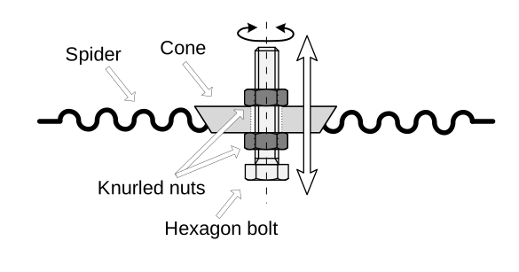
Attach the selected cone to the hexagon bolt using two knurled nuts.
Outer Clamping#
Select the outer clamping rings (refer to Selection of Clamping Rings for Outer Clamping)
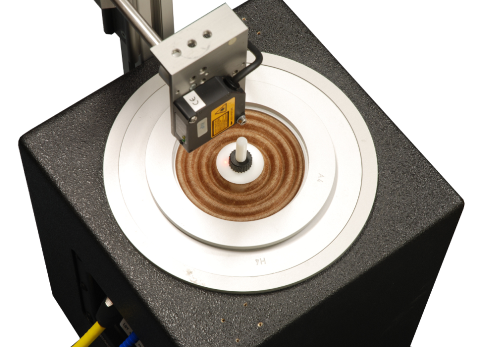
Once a suitable ring set is found it can be attached to the LST Bench. The outer diameter of the largest ring of each set (ring #5) fits the circular opening on top of the LST Bench.
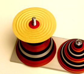
Place the suspension part on the rings as can be seen on the picture above. Put the inner clamping part carefully into the center of the DUT and place the upper clamping ring on the outer suspension rim.
Clamping Part Look-up Tables#
Ring Set for Outer Clamping#
Name of the ring |
\(D_{\text{R}}\) (mm) |
Name of the ring |
\(D_{\text{R}}\) (mm) |
|---|---|---|---|
A1 |
30 |
E3 |
103 |
B1 |
33 |
F3 |
108 |
C1 |
36 |
G3 |
113 |
D1 |
39 |
H3 |
118 |
E1 |
42 |
A4 |
124 |
F1 |
45 |
B4 |
130 |
G1 |
48 |
C4 |
136 |
H1 |
51 |
D4 |
142 |
A2 |
54 |
E4 |
148 |
B2 |
57 |
F4 |
154 |
C2 |
61 |
G4 |
160 |
D2 |
65 |
H4 |
166 |
E2 |
69 |
A5 |
173 |
F2 |
73 |
B5 |
180 |
G2 |
77 |
C5 |
187 |
H2 |
81 |
D5 |
194 |
A3 |
85 |
E5 |
201 |
B3 |
89 |
F5 |
208 |
C3 |
93 |
G5 |
215 |
D3 |
98 |
H5 |
222 |
Ring Set for Inner Clamping (SPM Bench)#
- 1 silver
- \(D_{\text{C}}\) in mm: 11\(D_{\text{U}}\) in mm: A1= 13.9; B1= 16.8; C1= 19.7
- 2 blue
- \(D_{\text{C}}\) in mm: 18\(D_{\text{U}}\) in mm: A2= 20.9; B2= 23.8; C2= 26.7
- 3 red
- \(D_{\text{C}}\) in mm: 25\(D_{\text{U}}\) in mm: A3= 27.9; B3= 30.8; C3= 33.7
- 4 gold
- \(D_{\text{C}}\) in mm: 32\(D_{\text{U}}\) in mm: A4= 34.9; B4= 37.8; C4= 40.7
- 5 black
- \(D_{\text{C}}\) in mm: 39\(D_{\text{U}}\) in mm: A5= 41.9; B5= 44.8; C5= 47.7
- 6 silver
- \(D_{\text{C}}\) in mm: 46\(D_{\text{U}}\) in mm: A6= 48.9; B6= 51.8; C6= 54.7
- 7 blue
- \(D_{\text{C}}\) in mm: 53\(D_{\text{U}}\) in mm: A7= 55.9; B7= 58.8; C7= 61.7
- 8 red
- \(D_{\text{C}}\) in mm: 60\(D_{\text{U}}\) in mm: A8= 62.9; B8= 65.8; C8= 68.7
- 9 gold
- \(D_{\text{C}}\) in mm: 67\(D_{\text{U}}\) in mm: A9= 69.9; B9= 72.8; C9= 75.7
- 10 black
- \(D_{\text{C}}\) in mm: 74\(D_{\text{U}}\) in mm: A10= 76.9; B10= 79.8; C10= 82.7
- 11 silver
- \(D_{\text{C}}\) in mm: 81\(D_{\text{U}}\) in mm: A11= 83.9; B11= 86.8; C11= 89.7
- 12 blue
- \(D_{\text{C}}\) in mm: 88\(D_{\text{U}}\) in mm: A12= 90.9; B12= 93.8; C12= 96.7
- 13 red
- \(D_{\text{C}}\) in mm: 95\(D_{\text{U}}\) in mm: A13= 97.9; B13= 100.8; C13= 103.7
- 14 gold
- \(D_{\text{C}}\) in mm: 102\(D_{\text{U}}\) in mm: A14= 104.9; B14= 107.8; C14= 110.7
Ring Set for Inner Clamping (LST Bench)#
- Cone 1
- \(D_{\text{C}}\): 11 mmWeight: 2.1 g
- Cone 2
- \(D_{\text{C}}\): 18 mmWeight: 5.2 g
- Cone 3
- \(D_{\text{C}}\): 25 mmWeight: 9.5 g
- Cone 4
- \(D_{\text{C}}\): 32 mmWeight: 14.9 g
- Cone 5
- \(D_{\text{C}}\): 39 mmWeight: 21.3 g
- Cone 6
- \(D_{\text{C}}\): 46 mmWeight: 28.9 g
- Cone 7
- \(D_{\text{C}}\): 53 mmWeight: 37.6 g
- Cone 8
- \(D_{\text{C}}\): 60 mmWeight: 47.3 g
- Cone 9
- \(D_{\text{C}}\): 67 mmWeight: 58.3 g
- Cone 10
- \(D_{\text{C}}\): 74 mmWeight: 70.1 g
- Cone 11
- \(D_{\text{C}}\): 81 mmWeight: 83.1 g
- Cone 12
- \(D_{\text{C}}\): 88 mmWeight: 97.3 g
- Cone 13
- \(D_{\text{C}}\): 95Weight: 112.4 g
- Cone 14
- \(D_{\text{C}}\): 102Weight: 128.6 g
- Hexagon Bolt
- Weight: 7.25 g
- Knurled Nut
- Weight: 3.25 g
Laser Calibration#
Warning
CAUTION LASER RADIATION! Avoid direct or indirect (e.g. reflection) exposure of human eyes to beam!
After the hardware installation it is required to check the laser calibration. The KLIPPEL Analyzer Hardware manual describes how to
Verify the calibration and
Calibrate the laser
Please see the KLIPPEL Analyzer Hardware manual section Calibration and Verification for further information.
Measurement of the Nonlinear Stiffness (SPM Pro)#
The Suspension Part Measurement is used to measure the nonlinear stiffness of suspension parts and passive radiators. The measurement procedure is based on a two-step process to automatically adjust the stimulus to measure the nonlinear stiffness at a specified target displacement. The operation relies on the Transfer Function Measurement (TRF) module to generate the stimulus.
Stimulus adjustment stage: During this phase the frequency range of the exciting sweep and the voltage is adjusted until a specified target displacement is reached. The current stimulus settings applied to the SPM bench is shown in the window Table Results. The running measurement can be canceled at any time by pressing the Cancel button
.Main measurement: This step is performed as soon as the optimal frequency range and target displacement is achieved. Depending on the measurement mode this step is performed once, repeated until a specific time elapsed or repeated infinitely.
Property Page#
Category “Input”#

- Moving Mass
- Unit: in gRange: > 0
Mass of the DUT with clamping parts
Category “Routing”#
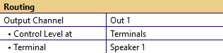
- Output Channel
- Options: Out 1, Out 2
Apply stimulus to the selected output channel.
Note
For KA3, the output channel depends on the available cards!
- Control Level at
- Options: Out, Terminals
Channel where the specified start voltage is applied.
- Terminal
- Options: Speaker 1, Speaker 2
Speaker channel of the analyzer device that is connected to SPM bench.
Note
This is only shown if Control Level at is set to Terminals.
Category “Measurement Setup”#
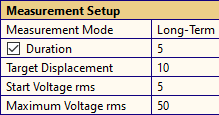
- Measurement Mode
- Options: Single, Long-Term
Select SPM measurement mode.
Single will perform a single measurement at target displacement,
Long-Term repeats the measurement at target displacement indefinitely or until a specified time has elapsed
- Duration
- Unit: minRange: > 0
Total measurement duration in “Long-Term” mode. After the specified target is reached, the measurement at target displacement will be repeated until the specified time has elapsed.
- Target Displacement
- Unit: mmRange: > 0
- Start Voltage rms
- Unit: VRange: \(0 < U_{\text{start}} < \ U_{\max}\)
Voltage of the first TRF measurement.
- Maximum Voltage rms
- Unit: VRange: > 0
Voltage limit for protection. Consider the voltage limit of the driving speaker!
Note
This is an advanced option and will only be displayed if Show Adanced Options is selected.
Category “Processing”#

- Number of Harmonics
- Options: automatic, 3, 5
Number of Harmonics used for \(K(x)\) calculation. 3 should be sufficient for spiders and 5 is recommended for cone-surround-assemblies or passive radiators.
Category “Export”#
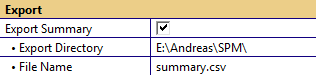
- Export Summary
Print results of main measurement in to a CSV summary file.
- Export Directory
Directory of CSV file into which the results are printed.
- File Name
Name of the CSV file into which the results are printed.
Category “Advanced”#

- Show Advanced Options
Shows advanced options: Maximum Voltage and Keep all data
- Keep all data
Leaves all interim TRF operations in the database.
Results#
Result Windows#
K(x) Stiffness#
The window shows the identified nonlinear stiffness \(K(x)\) of the DUT. The curve is based on a (regular) power series following the form
Depending on the number of harmonics used for the calculation a 2nd order power series (parabola) is calculated using three harmonics and a 4th order power series is calculated using five.
\(K(x)\) shows the nonlinear stiffness
\(K(-x)\) shows the nonlinear stiffness mirrored at the rest position \(x = 0\)
\(k_{\mathrm{eff}}\) shows the effective stiffness at the frequency of the displacement maximum
C(x) Compliance#
This window shows the compliance \(C(x)\). It is the inverse of stiffness \(K(x)\)
\(C(x)\) shows the nonlinear compliance
\(C(-x)\) shows the nonlinear compliance mirrored at the rest position \(x = 0\)
\(c_{\text{eff}}\) shows the effective compliance at the frequency of the displacement maximum
F(x) Force-Deflection#
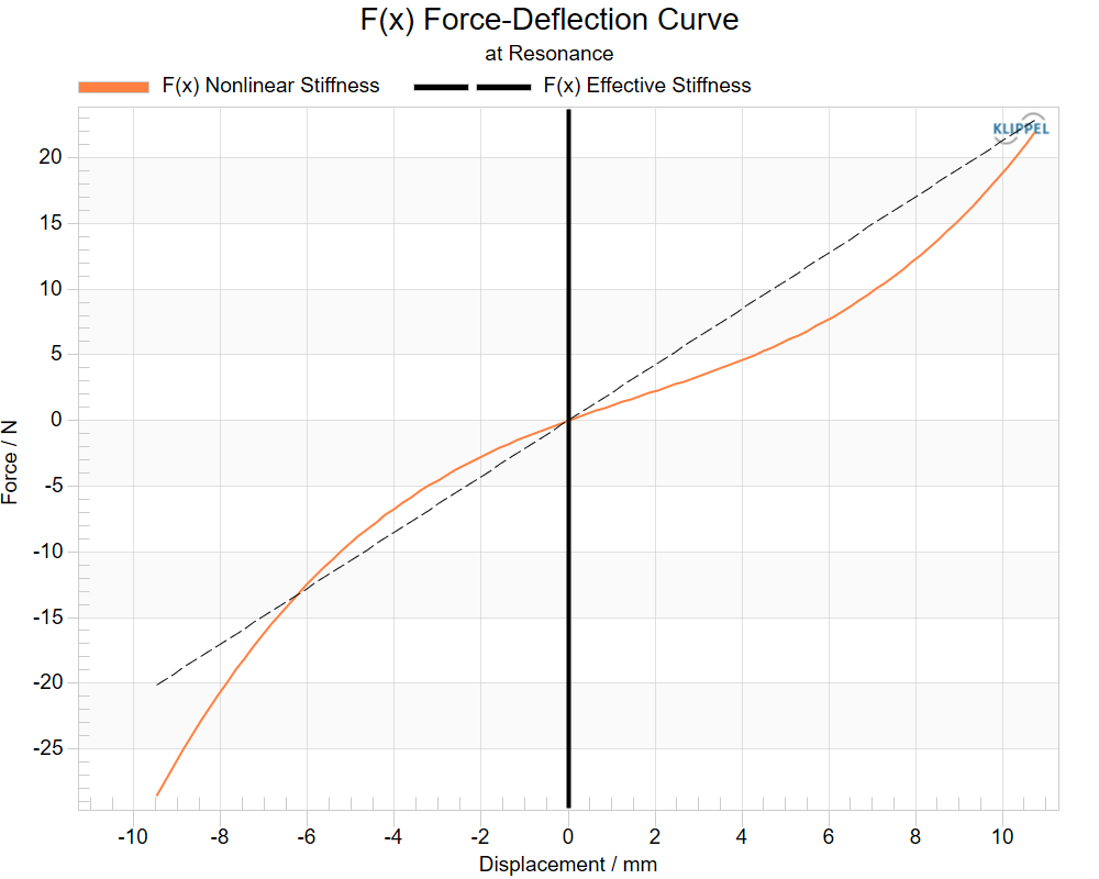
The window shows the stiffness force depending on the displacement produced by the DUT.
F(x) Nonlinear Stiffness shows the force deflection curve of the force produced by the nonlinear stiffness
F(x) Effective Stiffness shows the effective force deflection curve if the stiffness would be linear and equal to the effective stiffness (\(F_{k,\mathrm{eff}} = k_{\mathrm{eff}}x\))
x(t) Displacement Waveform#
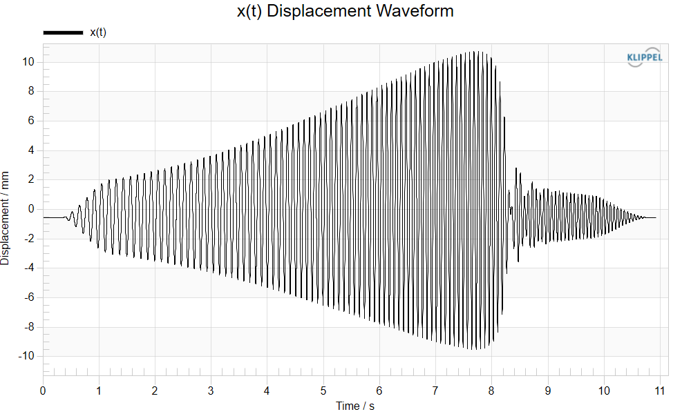
The window shows the measured displacement time signal of the sine sweep.
x(t) Displacement (Single Period)#
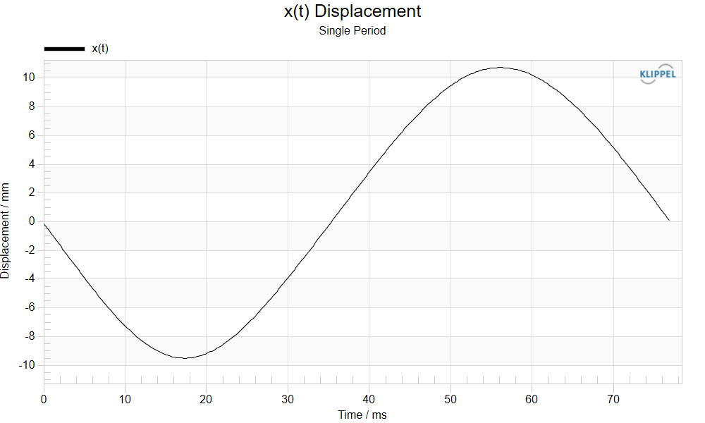
The window shows the section of the measured displacement time signal which is used to calculate the stiffness. A single sine period is selected where the displacement maximum occurs.
X(n) Displacement Overtone Spectrum#
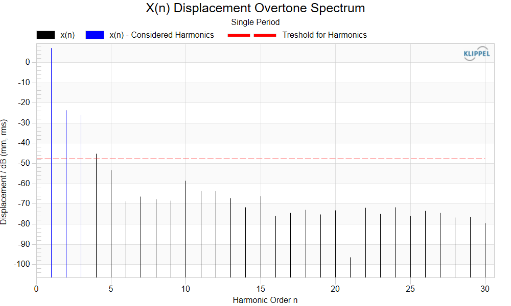
The window shows the overtone spectrum of the selected sine period section which is used for calculation. The level of displacement of the fundamental and its harmonics is visualized here. The dashed red line represents a noise threshold for harmonics. The harmonics used to calculate the results are visualized by blue lines.
F(t) Force Waveform (Single Period)#
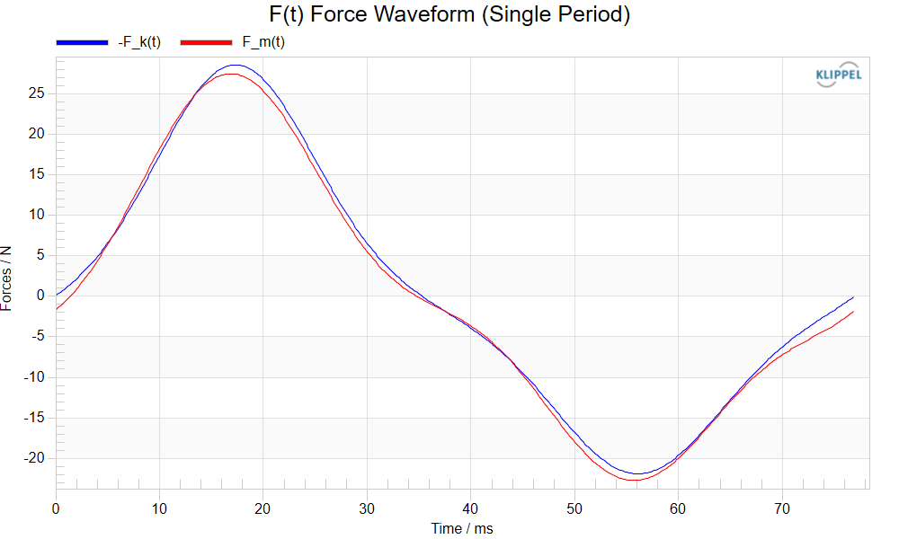
The window shows the time signals of the force produced by the mass and the inverse of the force produced by the stiffness. Only the section of the single sine period at resonance is shown, where the two forces should add up to zero if the quality of the identification of the stiffness is related to how good the two curves match.
Table Results#
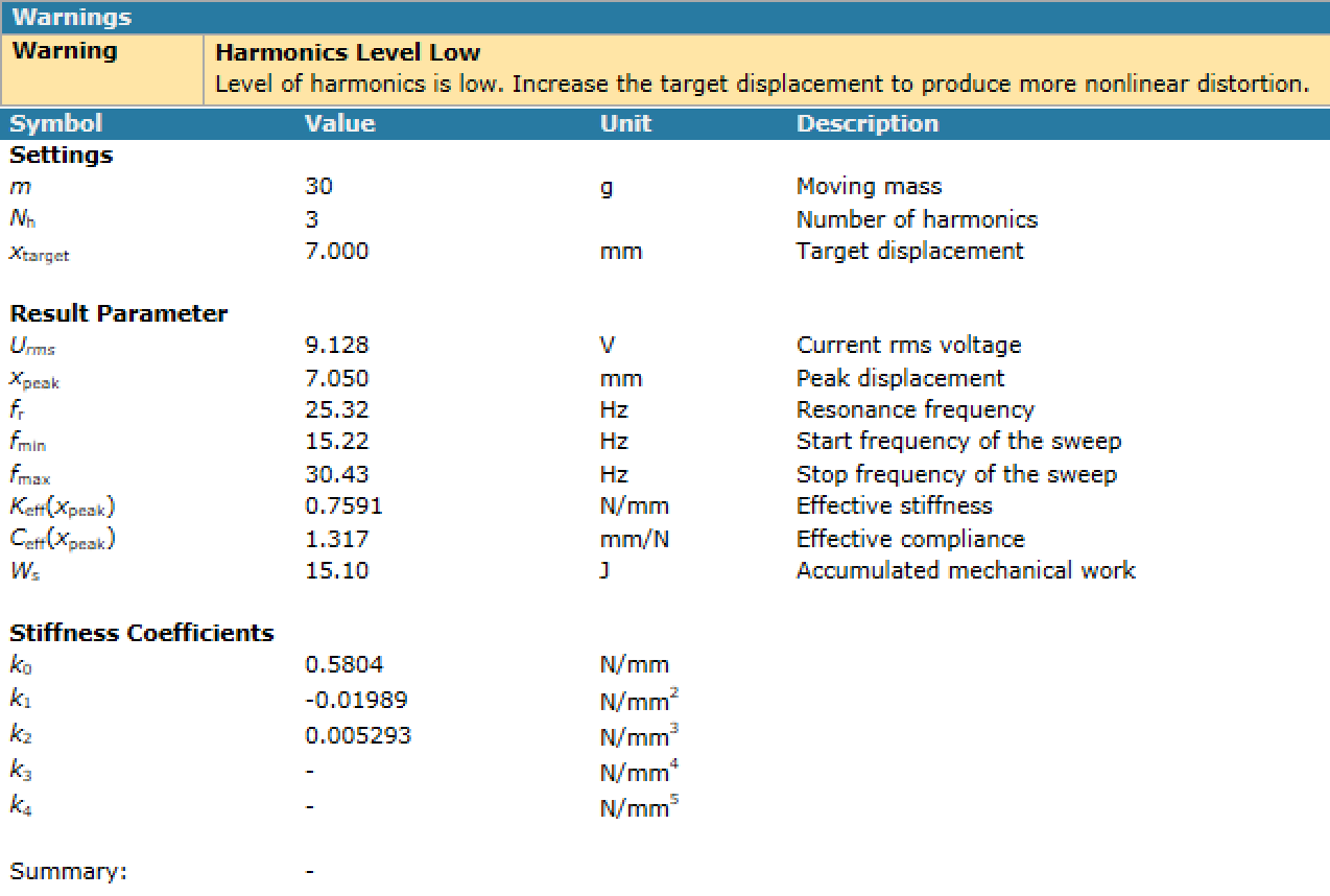
Measurement of the Linear Stiffness (SPM Lite)#
For the measurement of the linear parameters of suspension parts two templates for dB-Lab are provided. This template contains the following operations:
1 TRF Setup may be used to setup the measurement parameters (voltage, frequency range)
five TRF operations for the main measurements
If the used method is Added Mass also five TRF operations for the measurements with added mass
4 SPM Lite Suspension Part Measurement calculates the linear parameters based on the previous TRF operations
Measurement Principle#
The TRF operations stimulate the loudspeaker with a sine sweep so that the suspension part gets pneumatically excited. By measuring sound pressure and suspension part displacement simultaneously, the transfer function \(H_{\mathrm{x,p}}(\mathrm{j}\omega)\) is determined. Based on this function it is possible to determine the Q-factor and resonance frequency by fitting a resonator model. With the known parameter moving mass, the remaining linear parameters can be determined.
Two options are provided to measure the moving mass, from which the preferred one is the Added Mass Method. A piece of mass is added to the DUT and an additional TRF measurement is performed. Then the moving mass can be calculated by the two resonance frequencies and the value of the added mass. The second option is to weigh the suspension part including the inner clamping with a high precision scale.
The linear parameters are determined by the SPM Lite operation. This operation computes the Q-factor and resonance frequency \(f_{\mathrm{r}}\) by employing a suitable fitting algorithm. With the knowledge of resonance frequency, Q-factor and moving mass, the mechanical compliance and resistance are calculated.
Measurement Steps#
Clamping
Setting up the stimulus settings
Main measurements
Determining the moving/added mass
Selecting the measured TRF operations in the SPM Lite setup
Running the SPM Lite to calculate results
Clamping#
The clamping of the device under test is done as described in the section clamping in this chapter. If the SPM bench is used the guiding rod should be removed in order to perform a small signal measurement.
When using the LST bench please read the note about custom clamping in section LST Bench.
Setting Up the Stimulus#
Motivation: The \(K(x)\) nonlinearity is causing a variation of the suspension compliance which depends on the suspension part deflection. To make sure that this nonlinearity has only a negligible impact, the deflection has to be kept as small as possible. When setting up the stimulus settings for the measurements, the voltage should be as low as the SNR of the displacement laser signal allows it.
Also, the frequency range may be limited to decrease measurement time.
Note
If the highest magnitude in the measured \(H(f)\) curve does not occur at the resonance frequency \(f_{\mathrm{r}}\), limit the frequency range so that this condition is fulfilled (e.g.: \(\frac{1}{3} f_{\mathrm{r}} < f < 2.5 f_{\mathrm{r}}\)). Otherwise, the resonance frequency cannot be identified by the algorithm. This can be the case if the signal is corrupted by noise or parasitic vibrations.
The SPM Lite template contains the operation 1 TRF Setup which may be used to setup the stimulus. Its property page Stimulus provides options to modify voltage and frequency range.
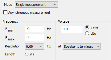
The voltage should be adjusted so that the suspension part displacement is small (< 1 mm). If the voltage was too small during the measurement it may happen that the measured curve is distorted as shown in the image below.
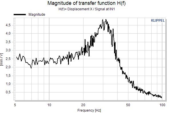
In this case the voltage has to be increased. It is advised to keep the SNR above 25 dB at the resonance frequency. This information can be found in the results window Y2(f) Input Spectrum.
Main Measurement#
The operations 2.1…2.5 TRF are dedicated to the main measurements. These are performed with the stimulus settings which were found in the last step. It is possible to perform up to five measurements which can be averaged to increase accuracy.
Determining the Moving Mass#
Two options to determine the moving mass are available: 1. the Added Mass Method and 2. weighing the suspension part mass using a scale which can be specified by the parameter Measurement Mode in the property page of the SPM Lite operation. The second option should only be chosen if the suspension part is very soft and the measurement is performed with the DUT mounted horizontally (e.g., on the top of the LST bench).
Added Mass Method#
An additional mass has to be attached to the suspension part. This can be done by screwing one or multiple nuts and if necessary, an additional cone from the cone set (27 or 44) to the sliding sleeve (SPM Bench) or the hexagon bolt (LST Bench). The mass should have a weight of around 50-100 % of the suspension part including the inner clamping parts. The value of the added mass has to be entered into the parameter Added Mass in the property page.
For the measurements use the operations 3.1…3.5 TRF (Added Mass). Perform at least one measurement, multiple measurements may increase the accuracy of the parameter identification. Perform the measurements with the same stimulus settings like in the main measurements.
Determining the Mass with aSscale#
In case the Added Mass Method should not be used, weigh the suspension part with the inner clamping with a high precision scale. In the next step this value is entered into the input variable Moving Mass.
Property Page#
Category “Input”#
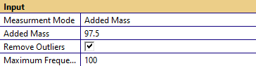
- Measurement Mode
- Options: Moving Mass, Added Mass
Specifies which method to use for the calculation of linear parameter. Moving Mass method uses the specified moving mass for calculations. Added Mass method calculates the moving mass from the resonance shift caused by an additional mass added to the DUT with clamping parts.
- Added Mass
- Unit: gRange: > 0
Additional mass that is attached during the measurements with Added Mass. This parameter is only available for Measurement Mode - Added Mass
- Moving Mass
- Unit: gRange: > 0
Mass of the DUT incl. clamping parts. This parameter is only available for Measurement Mode - Moving Mass
- Remove Outliers
This option excludes outliers of the imported transfer functions from the fitting.
- Maximum Frequency
- Unit: HzRange: \(0 \leq f_{\max} \leq 200\)
Maximum frequency used for the fitting of the transfer functions.
Category “Measurements without Mass”#
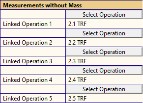
- Select Operation
Opens an operation selection dialog on button click.
- Linked Operation 1…5
Name of the operation selected with the Select Operation dialog. If the linked operation contains result data, the transfer function will be used to calculate the results. If more than one operation is specified the results will be averaged. An information message is displayed when the linked operation does not contain results.
Note
The linked operation needs to be in the same Object (driver) node as the SPM Lite operation.
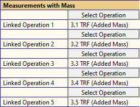
Category “Measurements with Mass”#
- Select Operation
Opens an operation selection dialog on button click.
- Linked Operation 1…5
Name of the operation selected with the Select Operation dialog. If the linked operation contains result data, the transfer function will be used to calculate the results. If more than one operation is specified the results will be averaged. An information message is displayed when the linked operation does not contain results.
Note
The linked operation needs to be in the same Object (driver) node as the SPM Lite operation.
Results#
Table Results#
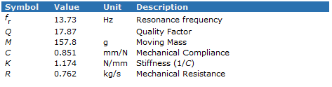
In this window the calculated linear parameters are shown. Also, error and warning messages appear in this window.
H(f) Magnitude Pos. 1…5#
These curves show the measured and the fitted transfer functions between sound pressure (microphone voltage) and displacement. The window H(f) Magnitude Pos. 1 corresponds to the operation linked in Linked Operation 1 in the category Measurements without Mass. It is useful to compare the measured and the fitted curves. The better they match around the resonance peak, the more accurately the parameters were determined.
Theory#
Basic Setup#
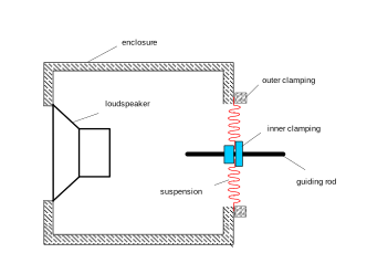
The outer rim (shoulder) of the suspension part is usually firmly clamped by using rings. The inner rim (neck) of the suspension is also clamped on a moving slide. This increases the moving mass \(m\) significantly. The stiffness \(K(x)\) and the moving mass \(m\) form a resonating system. At the resonance frequency the restoring force of the suspension equals the inertia of the mass. Due to the additional mass most of inertia acts directly to the neck of the suspension. Thus, the suspension is operated in a similar way as in a real loudspeaker. The suspension part is excited pneumatically by using a loudspeaker and an enclosure. The suspension is operated in vertical position to avoid any offset in the displacement due to gravity. An additional guiding rod for the slide may be used to prevent eccentric deformation of the suspension part and to suppress other vibration modes.
The nonlinear vibration of the suspension is measured and the unknown stiffness parameters are estimated by system identification techniques.
Acoustical Modeling#
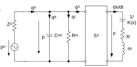
At low frequencies the setup may be modeled by the lumped parameter model shown above. The loudspeaker generates a volume velocity \(q_{\mathrm{D}}\)
where the volume velocity \(q_{\mathrm{B}}\) flows into the volume of the box, \(q_{\mathrm{L}}\) is leaving the box through leaks and the volume velocity \(q_{\mathrm{S}}\) produces the force \(F\) driving the suspension part under test.
The pressure \(p\) in the box generates a force \(F = S_{\mathrm{S}}\cdot p\) on the suspension part using an effective area \(S_{\mathrm{S}}\). In case of spiders the effective area \(S_{\mathrm{S}}\) has to be considered as a coupling factor between the acoustical and mechanical domain but is (due to the porosity) not identical with the geometrical area \(S_{\mathrm{geo}}\). For example, a spider may have a much smaller effective area (\(S_{\mathrm{S}} < 0.5\cdot S_{\mathrm{geo}}\)).
The acoustical compliance \(C_{\mathrm{AB}}\) depends on the volume \(V\) of the enclosed air and the static barometric air pressure \(p\).
The loudspeaker used for pneumatic excitation is modeled by an acoustical impedance \(Z_{\mathrm{D}}\) and a pressure source \(p_{\mathrm{D}}\).
The clamped suspension is described by the displacement \(x\) of the inner clamping part and the driving force \(F=S_{\mathrm{s}}\cdot p\) which is related to the sound pressure \(p\) in the test box. The driving force
is the sum of the restoring force \(k(x)\cdot x\) of the suspension, the force \(R\frac{\mathrm{d}x}{\mathrm{d}t}\) overcoming the friction of the guiding elements and the losses in the suspension material and the inertia accelerating the mass \(m\).
The moving mass \(m\) can be approximated by the total mass of suspension and the inner clamping parts.
Measurement of State Variables#
The identification of the parameters \(K(x)\) and \(k_{0}\) requires the measurement of some state variables such as force, displacement or pressure in the system.
The measurement of the displacement \(x\) is accomplished by a relatively inexpensive laser sensor based on the triangulation principle.
The sound pressure inside the box can be measured by using a normal microphone. However, the driving force \(F=S_{\mathrm{s}}\cdot p\) cannot be calculated in absolute values from the measured sound pressure \(p\) because the effective area \(S_{\mathrm{s}}\) of the suspension is usually not known.
Small Signal Behavior#
A sinusoidal sound pressure signal
produces a sinusoidal displacement
as long as the amplitude of the displacement is sufficiently small (\(X_1\approx 0\)) to ensure that the stiffness \(K(x) = k_0\) and resistance \(R\) are constant and the system behaves linearly. The transfer function between sound pressure and displacement
has a low-pass characteristic as shown as a thick line in the diagram below.
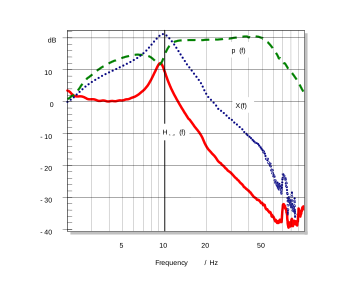
Magnitude response of the sound pressure \(p(f)\) (dashed line), displacement \(X(f)\) (dotted line) and the transfer function \(H_{\mathrm{x,p}}(f) = X(f) \cdot p(f)\) (thick solid line)
At the resonance frequency \(\omega = \omega_{\mathrm{0}}\) with
Since the losses of the suspension part and the friction of the clamping parts sliding on the rod are usually small, the transfer function \(H_{\mathrm{x,p}}(\mathrm{j}\omega)\) has a distinct maximum at resonance.
The size of the peak corresponds to the loss factor
which is usually high (\(Q > 2\)) and describes the ratio of the magnitude of \(H_{\mathrm{x,p}}(\mathrm{j}\omega)\) at resonance and at very low frequencies.
If the mass, resonance frequency and Q-factor are known, the small signal parameters can be identified. The moving mass can be determined by weighing the suspension part with inner clamping or using the Added Mass Method. By performing two measurements of the resonance frequency, once without added mass and once with added mass, the moving mass can be calculated.
Large Signal Behavior#
At higher amplitudes the varying stiffness \(K(x)\) generates a nonlinear vibration behavior of the suspension. For a sinusoidal excitation voltage, the sound pressure signal in the enclosure
and displacement of the inner rim of the suspension part
comprise a DC component \(X_0\), a fundamental component \(X_1\), \(P_1\) and harmonics \(X_i\), \(P_i\), at frequencies \(i\cdot \omega\) with the order \(i > 1\).
For sinusoidal excitation, the complex ratio \(H_1(\mathrm{j}\omega)\) of the fundamentals \(X_1\) and \(P_1\) in the displacement and sound pressure spectrum, respectively, may be expressed as
using the effective stiffness \(k_{\mathrm{eff}}\) which depends on the stiffness characteristic \(K(x)\) and the peak displacement \(x_{\mathrm{peak}}\).
At a particular frequency
the real part vanishes and \(|H_1(\mathrm{j}\omega)|\) becomes maximal if the mechanical losses represented by resistance \(R\) are sufficiently small.
The frequency \(\omega_{\mathrm{r}}\) may be understood as a large signal resonance frequency depending on the peak displacement \(x_{\mathrm{peak}}\) in contrast to the constant value \(\omega_0\) found in the linear model. Due to the low losses in the suspension and the high loss factor (\(Q > 2\)), the large signal resonance frequency may also be detected by searching for the maximum in \(|H_1(\mathrm{j}\omega)|\).
However, driving the system into resonance at high amplitudes is not as trivial as in the small signal domain. Since the effective stiffness usually increases with peak displacement \(x_{\mathrm{peak}}\) the large signal resonance frequency \(\omega_{\mathrm{r}}\) is usually much higher than the small signal resonance \(\omega_0\). Performing a sinusoidal sweep with falling frequency leads to a maximum at much lower frequencies than sweeping with rising frequency. The reason for this phenomenon is illustrated in the diagram below.
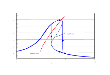
Due to the displacement depending resonance \(\omega_{\mathrm{r}}(x_{\mathrm{peak}})\) and the high \(Q\) there is a bifurcation into three states on the right side of the backbone curve whereas only two states are stable. Performing a sweep with rising frequency started one third-octave below the large signal resonance usually leads the nonlinear resonator into the upper state and the large signal resonance \(\omega_{\mathrm{r}}(x_{\mathrm{peak}})\) can be found where the ratio \(|H_1(\mathrm{j}\omega)|\) between the fundamentals becomes maximal. Performing a sweep with falling frequencies, the system usually uses the path via the lower states and the system actually misses the resonating state. A similar result may be obtained by exciting the suspension with a fixed frequency at \(\omega_{\mathrm{r}}\) by increasing the excitation amplitude slowly. The resonator remains in the lower state and finally at very high excitation or by any perturbation the resonator jumps into the upper state which is usually below resonance.
Measurement of the Parameters#
The suspension is excited by a sweep signal starting at least one-third octave below resonance ending approximately one-third octave above resonance. The displacement of the inner clamping parts and the sound pressure in the box are measured by sensors (laser triangulation sensor and microphone inside the box) and provided as time signals to the signal processing. For the measurement of spiders and smaller sized cones, the sound pressure measurement may be omitted and the ONE-SIGNAL-METHOD may be used as discussed in detail below.
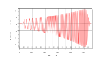
The diagram above shows the recorded displacement signal where the following nonlinear symptoms are found:
A characteristic decay (jumping effect) of the amplitude above resonance is clearly visible. Searching for a maximum in the displacement pressure ratio \(|H_1(\mathrm{j}\omega)|\) leads to the effective resonance frequency \(\omega_{\mathrm{r}}\) if the loss factor \(Q\) is greater than 2. The loss factor should always be checked to get an indication for bad clamping of the suspension and excessive friction at the slide on the guiding rod.
The dc-component is generated dynamically by the asymmetry of the stiffness and depends also on the amplitude. The dc component is also visible in figure above. At the beginning of the measurement the displacement is almost symmetrical but becomes asymmetrical at higher amplitudes. The bottom value (-17 mm) is at resonance \(\omega_{\mathrm{r}}\) much lower than the peak value (+11 mm).
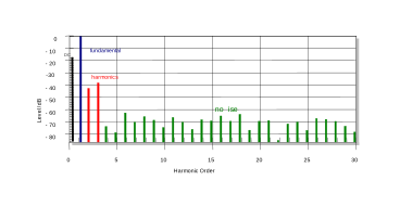
Harmonic Distortion can be found in the displacement signal. The diagram below shows the spectrum of one period of the displacement time signal located at the resonance frequency (maximal displacement of the sweep signal). The spectrum comprises a fundamental, a DC component, a 2nd-order and 3rd-order components which are clearly above the noise floor.
Effective Stiffness keff#
With known values of the effective resonance frequency \(\omega_{\mathrm{r}}\) and the moving mass \(m\) the effective stiffness
or the effective compliance
can be calculated. Since the resonance frequency \(\omega_{\mathrm{r}}\) depends on the amplitude, the effective stiffness should also be understood as a function of the displacement \(x_{\mathrm{peak}}\).
Nonlinear Stiffness K(x)#
More detailed information about the properties of the suspension gives the displacement varying stiffness \(K(x)\). The curve can be calculated from the nonlinear distortion found in the sound pressure and displacement signals.
The expression in equation of the driving force is the basis for the identification of the nonlinear stiffness. Considering that measured displacement and sound pressure signals are corrupted by noise and calibration errors, the balance of the forces in the resonator is written as the model error equation
The shape of the nonlinear \(K(x)\) characteristic is estimated by straightforward optimization where the squared error in the cost function
is minimized over a certain time interval \(T\). To search between a wide variety of candidates for the curve shape, \(K(x)\) is expressed by a truncated power series expansion
Since there is a linear relationship between the unknown coefficients \(k_i\) with \(i = 0, 1, … N\) and the error signal \(e(t)\), the coefficients can be estimated by searching for the minimum in the cost function in a \((N +1)\)-dimensional space by solving a linear set of equations
The model error equation still requires precise values for the additional parameters \(m\), resistance \(R\) and effective area \(S_{\mathrm{s}}\). While the moving mass \(m\) can easily be measured by weighing the suspension part with inner clamping, the resistance \(R\) and effective area \(S_{\mathrm{s}}\) cannot be measured directly. This problem can be solved by using a modified error equation developed as a Two Signal Method in [2].
This technique puts minimal requirements on the microphone used and still works if the microphone is not calibrated and has a poor amplitude response. Also, the position of the microphone inside the box and any time delay in the measurement path is not critical as long as the same position is used in the pre- and main-measurements. However, the microphone should behave linearly at the sound pressure amplitudes occurring in the test enclosure. The laser displacement sensor should be calibrated carefully.
For spiders and smaller sized cones, the sound pressure measurement can be omitted and the simple One Signal Method may be used. If the acoustical compliance of the test box is large in comparison to the compliance of the suspension part, then a simplified error equation can be used. A simple but reliable criterion for the validity of this method is the distinctness of the resonance peak found in the displacement frequency response \(X(f)\).
Resistance R#
In the small signal domain, the suspension with inner clamping is measured without using a guiding rod. According to the loss factor, the resistance
may be calculated by using the known mass \(m\), the resonance frequency \(\omega_{\mathrm{r}}\) and the measured transfer function \(H_{\mathrm{x,p}}(\mathrm{j}\omega)\).
Measurements at high amplitudes require some guidance of the inner clamping part. The emerging friction contributes to the measured resistance \(R\) so that the losses of the suspension cannot be measured separately. However, the suspension losses have only a small impact on the final loudspeaker performance for two reasons:
The flow resistance of the air passing the voice coil in the gap contributes significantly to the total mechanical \(Q_{\mathrm{ms}}\).
In a voltage driven loudspeaker system, the electrical damping dominates the total loss factor \(Q_{\mathrm{ts}}\).
Supported Modules for Im/Export#
Malfunction and Troubleshooting#
Overview#
This chapter will provide information that can help you solve common problems that occur with SPM measurements. Please contact KLIPPEL support in case you need assistance.
Error Messages (SPM Pro)#
Measurement bench not connected or amplifier gain to low.#
Reason:
The desired voltage could not be applied to the terminal of the SPM Bench
Solution:
Check the connection to the amplifier and SPM Bench. Make sure that the amplifier is turned on and provides sufficient amplification.
Low signal to noise ratio (SNR) of measured displacement.#
Reason:
The signal to noise ratio of the displacement signal during stimulus adjustment is lower than 5 dB.
Solution:
Check the laser displacement sensor for:
proper connection
optimal laser type
optimal distance to the target
sufficient reflection
or increase the start voltage.
Reason:
The signal to noise ratio at target displacement is less than 20 dB above the noise floor
Solution:
Increase the target displacement and check the laser displacement sensor for:
proper connection
optimal laser type
optimal distance to the target
sufficient reflection
Resonance frequency is below optimal range (reduce weight of inner clamping)#
Reason:
The resonance frequency is too low (<4 Hz).
Solution:
Reduce the mass of the inner clamping parts (using plastic nuts instead of metal nuts).
Resonance frequency is above optimal range (increase weight of inner clamping)#
Reason:
The resonance frequency is too high (>48 Hz).
Solution:
Increase the mass of the inner clamping material (add some nuts).
Could not realize desired target displacement.#
Reason:
The desired target displacement could not be realized, because the maximum voltage is reached.
Solution:
Increase the maximum voltage or decrease the target displacement.
Reason:
A problem with the laser may exist.
Solution:
Check the laser sensor for proper operation.
Reason:
The desired peak displacement may not be realized due to excessive friction on the rod.
Solution:
Check the clamping of the suspension part. Take care that the center of gravity is in the middle of the slide.
Remove the guiding rod to avoid stiction at low amplitudes.
Increase the moving mass to increase the loss factor of the mechanical resonator.
Reason:
Suspension parts operated at high amplitudes (at high “Target Displacement”) may become unstable. Thus, either the desired peak displacement “Target Displacement” or the frequency range (as internal setting) have not been realized after <number> iterations.
Solution:
Reduce parameter “Target Displacement” in the property page.
Displacement signal corrupted.#
Reason:
The sine period with the displacement maximum of the measured signal could not be determined.
Solution
Check the laser displacement sensor for:
proper connection
optimal laser type
optimal distance to the target
Stiffness curve is partially negative.#
Reason:
Some parts of the stiffness curve are negative. A small negative stiffness might be an artifact caused by laser nonlinearity.
Solution:
Increase the target displacement “Target Displacement” to operate in the linear range of the laser.
Note
Note that a negative stiffness can occur if the corrugation roles are compressed in radial direction while passing the rest position or at medium amplitudes. This happens only in surrounds as far as we have seen it. It results in an unstable region and bifurcates into two states.
Insufficient resolution of measured sine period.#
Reason:
Frequency resolution of one period of measured signals has not enough samples. This may be caused by high parasitic vibrations or a too high minimum excitation frequency F min.
Solution:
Check your measurement assembly. In most cases loose screws may cause vibrations of the assembly which are disturbing the measurement.
Warning Messages (SPM Pro)#
Level of fundamental is low.#
Reason:
The fundamental is not sufficiently above noise level.
Solution:
Check the displacement signal
Increase target displacement.
Level of harmonics is low.#
Reason:
Detected harmonics are not above noise level due to low nonlinearity.
Solution:
Increase target displacement
Level of 5th order harmonics is low.#
Reason:
The number of harmonics is set to 5, but 5th order harmonics are not sufficiently above noise level.
Solution:
Set Number of Harmonics in the input property page of operation 3 or automatic or increase the target displacement to produce more nonlinear distortion
Specified csv-file could not be opened! Creating new File with Name: <name>#
Reason:
The specified file is already opened by another program. A new file is created with the specified name <name>.
Solution:
Close any other programs that may have opened the specified file.
Error Messages (SPM Lite)#
Channel 1 is limiting.#
Symptom:
This error is generated by the TRF module and is caused by a clipping microphone.
Solution:
Decrease the stimulus voltage
If the resonance peak in the achieved \(H_{\mathrm{x}}(f)\) curve is distorted and an increase of the stimulus voltage is not possible, a shaping profile has to be defined to linearize the sound pressure spectrum.
No valid curve for the measurement without mass is available#
Symptom:
No curve is given for the measurement without mass.
No curve from which parameters can be derived is given.
Solution:
No valid curve for the measurement with mass is available#
Symptom:
No curve is given for the measurement with mass and no value of Added Mass is specified.
No curve from which parameters can be derived is given and no value of Added Mass is specified.
Solution:
Make sure that data have been passed
Specify a value for Added Mass.
The resonance frequency of the measurements with mass is higher than without mass.#
Symptom:
The measurement with added mass is not causing a decrease of the resonance frequency. This message can only appear if the Added Mass Method is used and the variable Added Mass is empty
Solution:
Make sure that the linked TRF operations are correctly assigned
The resonance frequencies with mass and without mass are identical.#
Symptom:
Apparently, the input curves are identical. This message can only appear if the Added Mass Method is used and the variable Added Mass is empty
Solution:
Make sure that you have inserted the correct curves into the input variables
Was a mass attached to the suspension part?
The frequency resolution around the peak of the transfer function is not sufficient.#
Symptom:
The frequency resolution is not sufficient to determine resonance frequency and Q-factor with adequate accuracy.
Solution:
Increase the frequency resolution to e.g.: 0.05 Hz. If necessary, select a smaller bandwidth by adjusting the upper/lower frequency limit.
Symptom:
The resonance frequency is too low (close to 3 Hz).
Solution:
Decrease the moving mass of the DUT and clamping.
Symptom:
The maximum of the magnitude transfer function is not determined correctly due to noise.
Solution:
Increase the signal to noise ratio by increasing the excitation voltage.
Warning Messages (SPM Lite)#
The following operations could not be found in the parent driver node or are invalid#
Reason:
The name of the linked operation may have changed, it was deleted or the operation is not a TRF.
Solution:
Repeat the select operation process of the invalidly linked operation or remove the linked operation.
The resonance peak of the transfer function was not determined correctly. This curve is not considered for the calculation.#
Symptom:
The particular curve is not suitable for the calculations.
Solution:
Make sure that the highest magnitude occurs at the resonance frequency. Fix this by limiting the frequency range, using the input parameter Maximum Frequency or by defining a shaping profile.
If the curve does not look like a typical transfer function check the measurement setup.
Decrease the added mass to increase accuracy. / Increase the added mass to increase accuracy.#
Symptom:
The deviation between the resonance frequencies of the measurements with mass and without mass is too high. This message can only appear if the Added Mass Method is used and the variable Added Mass is empty.
The deviation between the resonance frequencies of the measurements with mass and without mass is too small.
Solution:
Repeat the added mass measurements a smaller/bigger mass. If you are sure that the weight of the added mass is suitable, make sure that the measured curves have been passed to the SPM Lite operation correctly.
The resonance frequency of the measurements without mass is very low. / The resonance frequency of the measurements with mass is very low.#
Symptom:
The resonance frequency is below 10 Hz.
Solution:
If possible, reduce attached mass to increase resonance frequency.
