SAN – Spectrum Analysis

SAN - Tutorial

Overview

The Spectrum Analysis (SAN) is a measurement task for the QC software framework of the KLIPPEL Analyzer System. It is included in the QC Standard Software package as well as in QC Basic Special Application version. For users of the R&D software framework a separate license is available.

The SAN is a universal tool for testing any kind of audio system input/output with as well as for general noise and vibration testing. In case the device under test (DUT) provides a signal input, the internal pink/white noise generator of the SAN can be used to measure characteristics like sound pressure spectrum, frequency response, A- and C-weighted level and incoherence (distortion). Additionally, a user-defined custom stimulus signal can be imported as an audio file instead.

Even when no test signal can be applied, the spectrum and level of any sound or noise sources can be tested using PASS/FAIL limits.

Note

The SAN replaces the discontinued Coherence (COH) task, but with restricted data compatibility. In order to ensure trouble-free transition, the update is not performed automatically - the COH tasks will be still delivered together with the normal software distribution for a limited time. In order to use the SAN, new QC tests shall be created based on new test and operation templates. Alternatively, a manual update trigger is provided in the COH.

What is the Goal of This Tutorial?

This tutorial is dedicated to make you familiar with setting up and using the SAN for two typical test scenarios:

1. Noise & vibration testing (passive measurement)

2. Audio system testing (with test signal stimulus)

The tutorial is divided into the following steps that consider the specifics of both applications

• Setting up the hardware

• Creating a SAN test

• Adjusting most important settings

• Performing a first measurement

• Viewing results

• Testing with limits

• Working with custom test signals

Hardware Setup

The required hardware components for a SAN test very much depend on the test scenario. The picture below shows a generalized schematic test setup for noise & vibration testing as well as audio system testing applications based on KLIPPEL Analyzer 3 (KA3) QC Card version or an external sound card, alternatively.

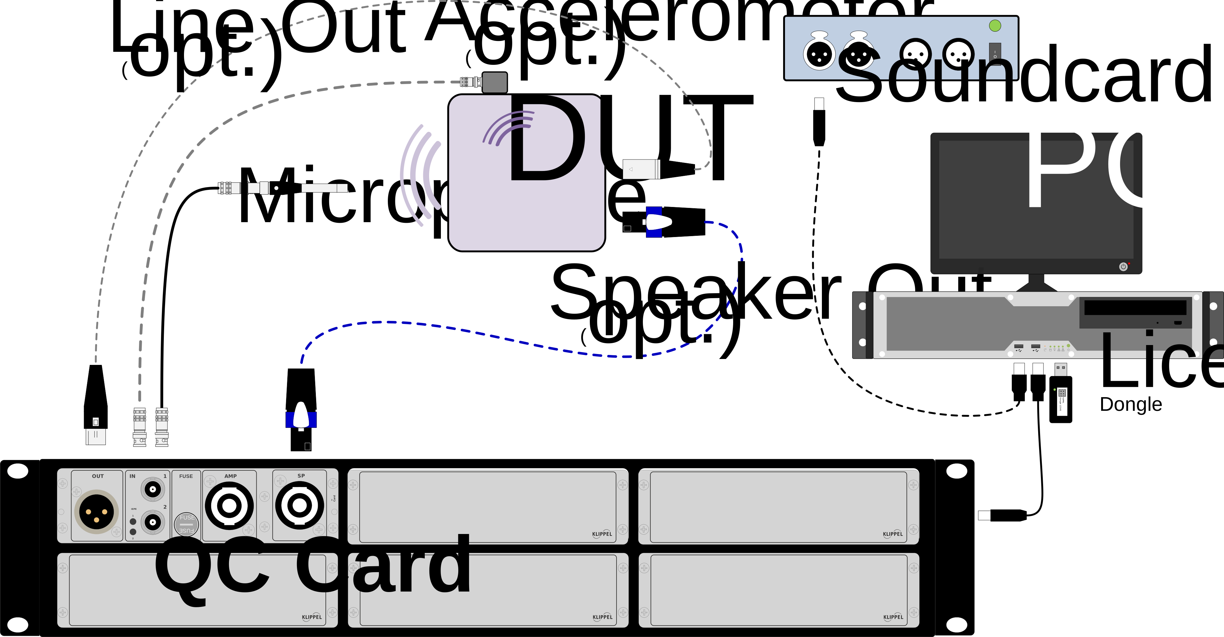
Setup for Noise & Vibration Testing

For noise and vibration testing of machines, acoustic signaling devices and other noise sources, typically no signal input is available in the device under test (DUT). Only the sensor input (either sound pressure or acceleration) shall be tested and thus no test signal generator is required. Both, the microphone and/or accelerometer with IEPE supply can be connected directly to the microphone inputs of the KA3 (QC Card or Laser Card). Alternatively, a 3^rd party USB audio interface can be used for data acquisition using QC Stand-alone Software version.

Setup for Transfer Function Testing

For testing transfer characteristics such as frequency response or incoherence of audio systems (e.g. active loudspeaker, microphone response of Bluetooth® enabled headphone) a dedicated test signal is required.

Passive Devices

For passive devices (driver, speaker box), the DUT is connected to the Speaker output of the QC Card or the Speaker Card. Either the internal amplifier (QC Card or Amplifier Card) or an external amplifier may be used if power or peak voltage requirements exceed the specifications.

Active (Self-Powered) Devices

Active systems can be connected to any signal output of the analyzer, such as the XLR Out of the QC Card. For testing digital (USB) or wireless devices such as Bluetooth enabled speakers or headphones, the corresponding WDM sound device can be selected directly as playback device in the hardware configuration of the QC operation. Refer to general QC User Manual for more information. Automatic Bluetooth pairing and sound device control is provided by the optional External Devices Task (EXD Bluetooth).

Stand-alone Devices (Open Loop)

If no direct streaming is possible, an open loop scenario with stand-alone playback can be realized using External Synchronization (SYN) add-on that is fully compatible with the SAN. The test stimulus is exported to an audio file and transferred to a playback device such as a mobile phone or uploaded to a cloud service for smart device testing. An optional synchronization and trigger signal may be added. In SYN - Open Loop mode the SYN will trigger measurement automatically as soon as the audio file is played back.

Signal Configuration and Sensor Calibration

If you are using a KA3, make sure that the signal configuration (global assignment of inputs and outputs) is set according to the desired hardware setup. Refer to Hardware Manual for more information.

In case sensors such as microphones or vibration sensors are used, make sure that the stored sensor sensitivity and max level information is valid. Refer to QC Manual section Calibration / Check of Accuracy for more information.

Creating a SAN Test

QC Software Framework

Creating a New QC Test

1. Open the QC Start - Engineer

2. Click Test ‣ New…

3. Give the test a clear name and choose a base template (e.g. Default), then click Ok.

4. You may log into the test now by clicking the Measure button.

The following test templates are based on or include SAN:

• System Test (Pink Noise) – general test template for active (or passive) speaker, headphone or audio system

• Spectrum Test (SAN) – general test template for noise & vibration testing based on spectrum and A-weighted level (without test stimulus generator)

• Bluetooth Headphone (ANC) – for test noise attenuation using noise signals

Adding the SAN Task

Follow these steps to add a new SAN task to your existing test sequence. Skip this step if you have selected a test template that already includes SAN.

• Start the QC Test;

• click the Add… button in the Tasks section of the property page to add a new task.

  

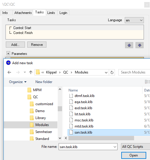
• Choose the task file san.task.klb. The default location is

  %ProgramData%\Klippel\QC\Scripts\Klippel\QC\Modules
  

• The SAN task will be added to the list of measurement tasks.

Note

Adding a new task always requires creating new reference units. You have to confirm that you want to delete all reference measurements, if limits exist in your test.

R&D Software Framework

If you are operating the SAN within the KLIPPEL R&D Software framework, you may add a QC SAN operation by using the provided operation template.

• Create or open a KLIPPEL database file

• Add a new operation by using the operation icon or Edit ‣ New Operation…

  

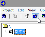
• Select Categories and Modules ‣ QC quality control and Templates ‣ QC Spectrum Analysis (SAN). Alternatively, you may enter SAN in the filter input field to quickly find the template.

• Choose a name and click OK to create a new QC operation

• Click Run to log in

See dB-Lab Software Manual for more information.

Performing a Noise & Vibration Measurement

Basic Settings

Before starting your first measurement, make sure that the basic test settings are configured correctly.

First set the global input routing in Control:Start - Routing properties. Output routing should be set to OUT in order to avoid conflicts of amplifier check. Now select Spectrum Analysis task to edit the remaining test settings.

Stimulus & Acquisition

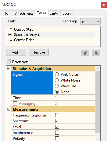
For testing without any dedicated test stimulus signal, the Signal setting shall be set to None in order to prevent any signal output. Selecting this mode, the SAN properties will be reduced to only a few options.

The parameter Time defines how long the sensor data shall be captured. The value indirectly defines the maximal achievable spectral resolution (using Result Frequencies - Full resolution setting).

Note

When using full resolution spectrum, the test time is limited to max. 4 s. In general, it is recommended to choose any other option than Full resolution in Processing – Result Frequencies in order to reduce data size, processing time and to improve result reproducibility at all frequencies.

Results

In this category, only two test result are available when testing without stimulus signal. Spectrum corresponds to the FFT spectrum of the captured sensor data.

Level corresponds to the total input level of the captured signal as a single value. Frequency weighting (A- and C-weighting) can be applied optionally (Processing ‣ Level - Mode).

Refer to Viewing Results and Definition of Results for more information.

The Measurement

After adjusting basic settings, you may start the test by clicking the Start button in the QC Control Panel. No test signal should be audible and after the specified capture Time, the results are displayed.

Viewing Results

Level

Activate Summary window to view single value result tables including Input Level result.

Input Spectrum

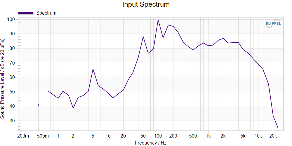
The FFT spectrum of the captured voltage or sensor input is displayed according to selected target resolution in Input Spectrum window. The full available frequency range is displayed if not specified otherwise in Display settings. The lower frequency end is defined by measurement Time while the upper frequency limit is set by the selected sample rate (Nyquist frequency). Find more information in section Definition of Results.

Note

Both, absolute level and frequency characteristic are affected by output resolution setting. It is recommended to use relative resolution (points per octave) instead of full resolution to avoid level dependency vs. test time.

Performing a Frequency Response Measurement

Basic Settings

Make sure that the global input and output routing in Control:Start - Routing properties are set according to your hardware setup and the configuration selected in corresponding Signal Configuration dialog. Refer to QC Manual sections Routing / Delay / GPIO Control for more information. Select Spectrum Analysis task to edit the remaining test settings.

Stimulus & Acquisition

Signal

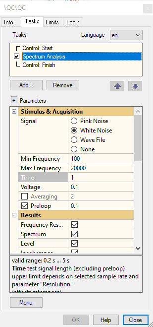
First, select a test stimulus Signal. Use the internal noise generator for pink or white noise signals or a custom WAVE file stimulus.

Note

For measurement of frequency response and incoherence using custom WAVE file stimulus it is recommended to use dense broad band signals to ensure proper signal-to-noise ratio in the tested frequency range. Refer to section Working with Custom Test Signals for more information.

White Noise generates a noise signal with constant absolute power spectral density in the specified frequency range, While Pink noise has a 1/f characteristic (constant relative spectral density).

Min./Max. Frequency

In case the noise generator is selected, you need to define an upper and lower frequency limit for the excited bandwidth.

Note

The specified min/max frequencies define the generator bandwidth only. Therefore, the result frequency range may differ slightly when using reduced resolution, since only fully excited frequency bands are displayed. However, the effective display frequency limits for the selected result resolution are shown in the parameter comments of Min. Frequency and Max. Frequency so you can adjust the generator bandwidth to achieve the desired result frequency range.

For custom stimuli, the effective bandwidth is a result of the spectral content and specified Dynamic Range setting (see section Stimulus Spectrum & Dynamic Range).

Time

The parameter Time defines the length of the main measurement (excluding Preloop) and indirectly determines the maximal available spectral resolution when using Full resolution.

Note

When using full resolution spectrum, the test time is limited to max. 4 s (@ 48 kHz). In general, it is recommended to selected any other option than Full resolution in Processing – Result Frequencies in order to reduce data size, processing time and to improve result reproducibility at all frequencies.

Voltage

The Voltage setting defines the effective voltage at the selected output terminal or at the amplifier output (depending on Output routing). For any given generator signal, the value corresponds to the overall RMS value of the complete signal (without Preloop).

Warning

Depending on the test signal’s crest factor, the peak voltage value may be significantly higher than the RMS value. Consider this for avoiding overload damage and for output and amplifier headroom.

For digital output devices (e.g. Bluetooth device or sound card), the output level is specified in dB FS instead.

Results

In addition to Level and Input Spectrum, further result parameters are available when using a known test stimulus that allows estimating the transfer behavior of the DUT. Frequency Response and Polarity (phase) are based on the measured linear transfer function, while Incoherence evaluates any non-linear behavior such as distortion.

The plain input spectrum and level parameters are still valid but they reflect both, stimulus characteristics and transfer behavior of the DUT.

The Measurement

After adjusting basic settings, you may start the test by clicking the Start button in the QC Control Panel. In acoustic tests, the noise or custom test signal should be audible and after the specified capture Time (+ Preloop), the results are displayed.

Viewing Results

Frequency Response

The Frequency Response describes the frequency-dependent transfer behavior between input and output of the audio system.

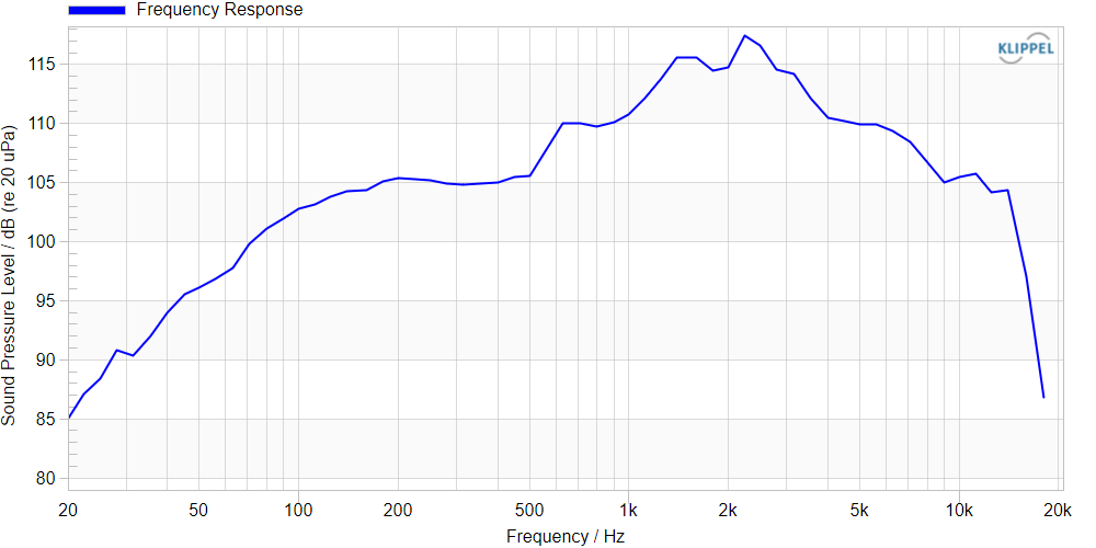
Two calculation modes are available (parameter Response – Mode):

• The Transfer Function is the magnitude of transfer function between DUT input and measured response spectrum. It is independent of the applied voltage for a linear system, but is affected by compression effects and thus depending on stimulus level in real DUTs.

• The SPL Frequency Response emulates the (sound pressure level) response to a sinusoidal signal with varying frequency (sweep) using the same RMS voltage. The frequency characteristic is identical to the transfer function but it reflects the absolute response level (e. g. sound pressure level) that depends on the stimulus level. Although it is not taking into account nonlinear system effects, it is basically comparable to the sine sweep frequency response measured by Sound Pressure (SPL) Task with the same RMS voltage (at small amplitudes). Find more information in section Definition of Results.

Polarity (Phase)

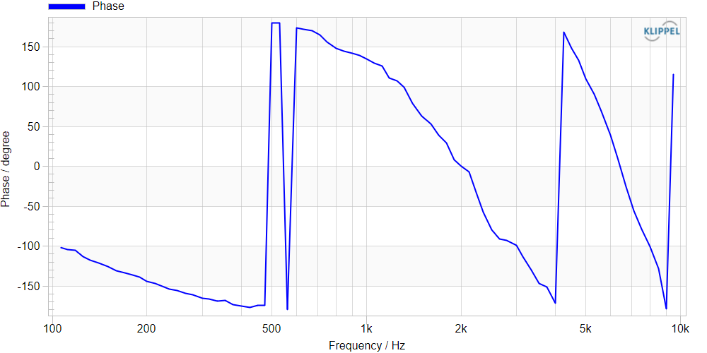
The Polarity test is based on the phase of linear transfer function at low frequencies. The actual test frequency is selected automatically during limit calculation based on average level, but it may be set manually instead.

Incoherence

The Incoherence is a very universal parameter for testing nonlinear distortion of audio systems (HD, IMD) with arbitrary test signals. It is derived from the magnitude squared coherence (difference to one) and can be displayed in percent or dB.

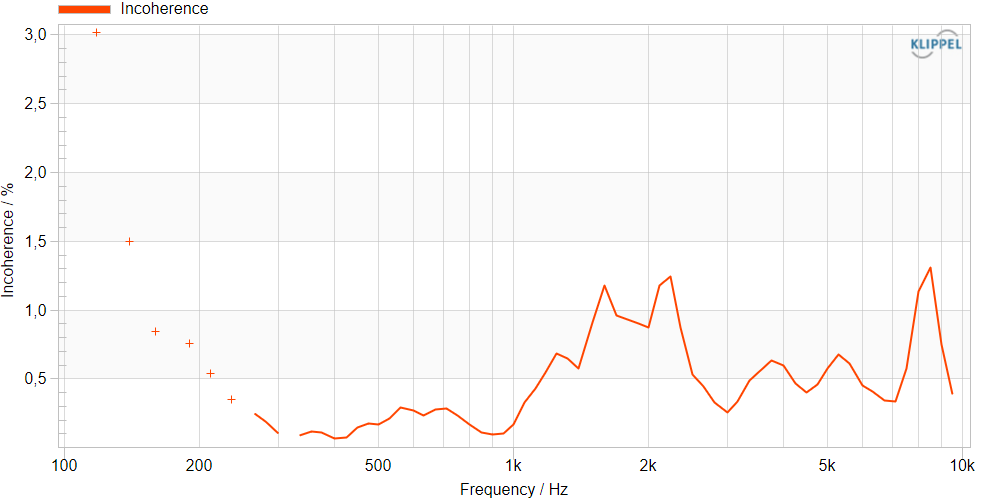
By definition, the (in)coherence is based on spectral estimation using average power spectra of the segmented, windowed output and input signals (Welch’s method). Therefore, the frequency resolution is lower compared to full resolution spectrum. This depends on the length of the time segments (Inco. – Window Length).

When using a defined output resolution, the frequency points will be identical in all curve results. However, the curve may be sparse at low frequencies due to the lack of primary data.

Note

The incoherence is not only a measure for nonlinear distortion of the DUT, but it will also reveal any additional noise introduced by the DUT, the sensors or the environment. Therefore, sufficient output is necessary at any tested frequency for sufficient SNR.

Testing with Limits

Setting Limits

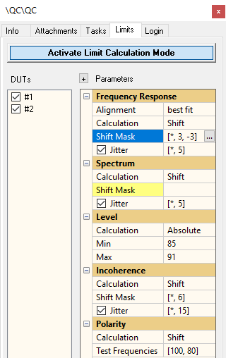
The limit handling of the SAN follows the general limit infrastructure of the QC software framework. For more detailed information, please refer to sections Reference Units and Limit Calculation in QC Manual.

Open your SAN test in Engineer mode select Limits tab on the Property Page and click Activate Limit Calculation Mode to access limit settings.

All test results measured in this mode will be stored as a reference unit that may be used for calculating relative limits. Individual result sets can be compared, deactivated or removed from the list.

Alternatively, absolute limits can be defined without using reference units. By clicking Calculate button (or leaving Limit Calculation Mode), the limits will be generated according to the selected calculation mode. The reference units are checked against those limits (Reference DUT Check) in order to detect outliers and a ranking of Golden DUTs will be displayed, if activated (see Golden Unit Handling).

The following limit calculation modes are available in the SAN:

Frequency Response

Modes: shift, statistic, absolute

Options: best fit alignment, jitter

Spectrum

Modes: shift, statistic, absolute

Options: jitter

Level

Modes: shift, statistic, absolute

Incoherence

Modes: shift, absolute

Options: jitter

Polarity

Modes: shift, absolute

Test Result

Once you have created limits, any tested DUT will generate a test verdict. If the results are within the tolerances, all tests will be passed and the Summary window will show a PASS overall verdict.

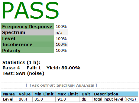
If the measurement result of a speaker violates the tolerance range, the failed parameter will be highlighted red in the Summary window. This results in an overall FAIL decision.

Limit Calibration

Like the Sound Pressure (SPL) task, the SAN supports Golden Units. Those special reference units are detected automatically in the reference DUT pool based on frequency response average. The highest ranked unit can be used to adjust the test limits anytime in case of systematic drifts changes of the test conditions (e.g. temperature). Please refer to QC Manual section Golden Unit Handling for more information.

Working with Custom Test Signals

Requirements and Basic Setup

The SAN allows importing arbitrary test signals in the Stimulus & Acquisition property page of the SAN.

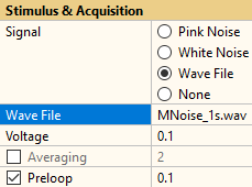
Virtually any signal can be imported from a WAVE file such as music or simulated program material. However, the following requirements apply:

• Sample rate must match QC Sound Device setting (Property Page ‣ Menu ‣ Configure Hardware…)

• Maximum length 20 s (less if Full Resolution used)

• Periodic signal desired

• Avoid signal waveform offset between signal start and end

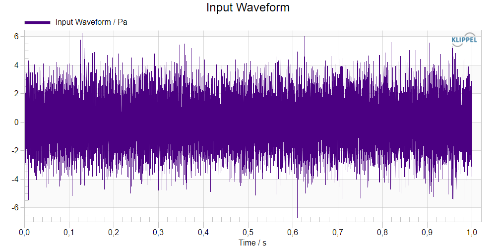
Further requirements apply for testing frequency response, phase and incoherence:

• The frequency spectrum should be dense

• The frequency bandwidth should cover the target test range (e.g., pass band of the DUT)

• The energy at all frequencies should be well distributed for optimal SNR (avoid strong level variation depending on frequency)

• A steady-state signal is desirable

See next section Stimulus Spectrum & Dynamic Range for more information.

Note

If the source file format is any other than .wav, you may use a 3^rd party format converter. An audio editor can be used to cut the source signal to the desired length.

The Voltage setting controls the playback gain based on the RMS of the full imported signal. Mind that the generated peak voltage and thus output or amplifier headroom may be significantly higher depending on the waveform’s crest factor.

A fade-in (Preloop) is recommended to avoid clicks and achieve stead-state conditions before the main response is captured.

Averaging can be used to improve signal to noise ratio. However, this increases test time significantly and should only be used with periodic (circular) signals.

Stimulus Spectrum & Dynamic Range

According to the requirements given in section Requirements and Basic Setup, the frequency content of the custom stimulus signal should be checked and the dynamic range needs to be defined to ensure valid and meaningful results for frequency response, polarity or incoherence. Those parameters shall only be tested at frequencies that are actually excited by the test signal, otherwise results are impaired by noise.

Note

For plain measurement of input spectrum or level, those requirements do not apply necessarily.

In order to view the imported signal’s spectrum, active Show Stimulus Spectrum in SAN – Display properties and open result window Stimulus Spectrum. One or two spectra are displayed in selected target resolution.

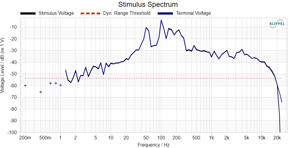
Stimulus Voltage corresponds to the ideal excitation voltage while Terminal Voltage represents the actually measured voltage spectrum at the DUT terminals (amplifier output). Deviations between both curves are normally caused by

• Amplifier frequency response (HF and LF roll-off)

• Finite output impedance of the amplifier (interaction with DUT load)

• Amplifier and sensor noise (at non-excited frequencies)

Note

Terminal Voltage is only available if a Speaker 1 1 or 2 routing is used and Reference parameter is set to Terminal Voltage.

In addition to the spectrum, a dynamic range threshold is displayed. This threshold ensures that the transfer behavior of the DUT is only tested at frequencies where the stimulus signal actually contains energy. All points where the stimulus spectrum magnitude is below this threshold will be omitted for all transfer-function-based results (frequency response, polarity and incoherence). Consequently, the affected result curves will be sparse as shown in the frequency response example below. The concerning frequency points are not removed (full frequency axis), but they do not carry a result value.

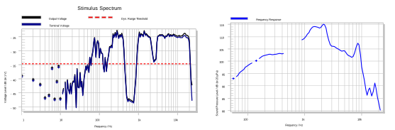
The threshold can be modified using the parameter Dynamic Range (Stimulus) in SAN Processing properties. This relative level in dB refers to the spectral maximum level. Increase/decrease this number to include/exclude stimulus frequencies with lower energy.

Note

If two few excited frequencies are found, a warning is generated.

Note

The target resolution (Result Frequencies) affects the dynamic range calculation and the number of valid results points significantly. Full resolution is not recommended due to the spectral fine structure. For incoherence, also the Window Length setting affects the effective frequency content.

Multi-Channel Data Aggregation

Some test applications require spatial averaging of multiple microphone’s responses. An example is measuring the audio system response inside a car using a microphone array instead of a single point measurement. For this purpose, the SAN provides the option to aggregate most of the test result parameter, such as frequency response based on multi-channel responses. Please refer to QC Manual section Multi-Channel Data Aggregation for more information.

Some features of the SAN are not compatible with multi-channel processing:

• Show Waveform display option

• Measurement of Incoherence

SAN – Reference

Task Parameters

The following parameters can be adjusted to customize this task.

Stimulus & Acquisition

Signal

Select the stimulus signal that shall be used for the SAN test

• Pink Noise

• White Noise

• Wave File

• None

“None” shall be used for tests without or with external excitation.

Note

Certain result parameters require a stimulus signal.

Min/Max Frequency[1]

Lower and upper frequency limit (bandwidth) of noise stimulus signal generator

Time[2]

test duration excluding Preloop

maximal allowed value depends on selected sample rate and parameter Resolution

Wave File[3]

Absolute or relative path to WAVE file with user defined stimulus

Note

Sample rate must match selected sample rate in QC hardware settings

Channel[3]

Select channel of WAVE file, if multiple channels available

Voltage, Voltage (Out)[4]

Test stimulus RMS voltage at the speaker terminals (amplifier output) or line output.

Availability depends on selected playback audio device and Output routing

Note

The realized voltage may be less than the specified voltage due to finite output impedance of the power amplifier.

Note

Peak value can be significantly higher depending on the selected stimulus!

Stimulus Level[4]

Peak stimulus level for digital audio devices in dB FS

Availability depends on selected playback audio device

Averaging

number of test loops for averaging (e.g. to improve SNR)

Note

Avoid this option when using non-periodic custom test signals (WAVE file) with inconsistent signal start/end

Preloop[4]

Preloop factor

relative duration of pre-excitation before measurement starts

Total excitation time = (1 + Preloop) ⋅ Time

Routing

Custom File for Import

path of task-specific custom WAVE file for processing (raw data import)

(only available in case of WAVE file processing)

Source Task

name and subtitle of SAN task used as signal data source for shared input signals (e.g. for multi-channel testing)

only visible if Execution - Allow signal data sharing is activated in Control Task.

See QC Manual section Signal Sharing for more information.

Output[5]

Output channel of the measurement hardware to be used:

• Speaker 1

• Speaker 2

• Out 1

• Out 2

• Out 1 + 2

Speaker 1 connect[5]

Connect terminal Speaker 1 to power amplifier output

only visible, if Routing / Output in Control Task is set to controlled by Task.

Speaker 2 connect[5]

Connect terminal Speaker 2 to power amplifier output

only visible, if Routing / Output in Control Task is set to controlled by Task.

Output Channel

select output channel(s) of playback device

(only available for 3^rd playback audio device output and if global Output is set to controlled by Task)

Input (Test Sensor) [6]

Input channel of the measurement hardware to be used:

• Mic 1

• Mic 2

• Line 1

• Line 2

• Mic linked to Speaker

• Line linked to Speaker

• Mic linked to Speaker (swapped)

• Line linked to Speaker (swapped)

only visible, if Routing / Output in Control Task is set to controlled by Task.

Test Sensor Input Channel

select channel of capture device or WAVE file for test sensor signal

Only available with 3^rd party capture device or Execution Mode - Load Input Signals and if Test Sensor Input is set to controlled by Task

Note

For re-processing exported WAVE file data (see Qc Manual section Save Input Signals) use channel #1

Additional Channels (Test Sensor)

Select additional channels for Multi-Channel Data Aggregation.

Only available with 3^rd party capture device or Execution Mode - Load Input Signals and if Test Sensor Input is set to controlled by Task and Allow Multi-channel Aggregation is activated.

Voltage Input Channel

select channel of capture device or WAVE file for excitation voltage signal

Only available with 3^rd party capture device or Execution Mode - Load Input Signals

Note

For re-processing exported WAVE file data (see Qc Manual section Save Input Signals) use channel #2

Digital Output[5] [6]

Set GPIO before test.

only visible, if Routing - Output in Control Task is set to controlled by Task.

Delay Before[5] [6]

Delay before playback (after GPIO setting, if requested).

only visible, if Routing - Output in Control Task is set to controlled by Task.

Delay After[5] [6]

Delay after playback (after GPIO setting, if requested).

only visible, if Routing - Output in Control Task is set to controlled by Task.

Results

Frequency Response, Spectrum, Level, Incoherence, Polarity

dis-/enable result parameters individually

The corresponding limits can be disabled independent of this setting

Processing

Result Frequencies

Defines frequency points of result curves within measured frequency range

• R10, R20, R40, R80: preferred frequencies (ISO 266)

• By resolution (ref. 1 kHz): define resolution using standardized frequencies (ref. 1 kHz)

• By resolution: define resolution (relative to Start frequency) - use this mode for compatibility with previous versions of the QC software

Resolution

points per octave

number of result points

Response - Mode

Select calculation method for frequency response

• SPL Frequency Response: transfer function according to IEC 60268-21 (sound pressure)

• Transfer Function: plain transfer function based on excitation and response spectrum

See section Definition of Results for more information.

Reference

Select reference signal (denominator) for transfer function and incoherence calculation

• Stimulus: stimulus (output) spectrum

• Terminal Voltage: measured voltage spectrum at speaker terminals (recommended)

Only available if Speaker output routing used. See Transfer Function for more information.

Response - Smoothing

Part of octave for Frequency Response smoothing

no smoothing if value is empty

Spectrum - Smoothing

Part of octave for Spectrum smoothing

no smoothing if value is empty

Inco. - Smoothing

Part of octave for Incoherence smoothing

no smoothing if value is empty

Inco. – Type

Select display unit of Incoherence

• Level (dB)

• Percent (%)

Inco. – Window Length

windowed block length for Incoherence calculation

defines length (and number) of time segments used for averaged spectral density estimation (Welch’s method)

Available range: 2.7 ms to 341.3 ms

See Incoherence for more information.

Level - Mode

Set calculation mode for Level result

• RMS: root mean square of total input signal. Unweighted level, also referred to as Z-Weighting.

• A-Weighting: weighted SPL according to IEC 61672 for lower and medium levels

• C-Weighting: weighted SPL according to IEC 61672 for higher levels

Curve Weighting

Apply pre-defined or custom input weighting curve to the frequency response, input spectrum or transfer function

• Off

• A-Weighting: weighted according to IEC 61672 for lower and medium levels

• C-Weighting: weighted according to IEC 61672 for higher levels

• Custom

Custom Curve

Custom weighting curve in dB

Format: [freq weight]

Only available for Curve Weighting – Custom

Invert

Inverts entered Custom Curve

Only available for Curve Weighting – Custom

Dynamic Range (Stimulus)[3]

dynamic range threshold of custom stimulus signal (for transfer function and incoherence calculation)

It is defined relative to the peak value of the excitation signal spectrum; only frequency points above the threshold are analyzed

See Stimulus Spectrum & Dynamic Range for more information.

Input Gain 1

Input preamplifier gain for Mic 1 and Line 1 input to optimize SNR

Note

Negative input gain cannot compensate overload of analog input stage. Effective range and available gain steps depend on used analyzer/card, please refer to hardware specification

Recording Delay

Fixed delay of captured signal relative to generator in ms (in addition to effective delay)

Display

Frequency Response - Ymin/Ymax

Minimum/maximum display level in dB for Frequency Response window

if empty, auto scaled

Distortion - Ymin/Ymax

Minimum/maximum display level in dB for Frequency Response window

if empty, auto scaled

Input Spectrum – Xmin/Xmax

Minimum/maximum display frequency in Hz for result window Input Spectrum

if empty, auto scaled

Input Spectrum Ymin/Ymax

Minimum/maximum display level in dB for result window Input Spectrum

if empty, auto scaled

Show Input Waveform

Show full resolution waveform (DC removed) of the measured input signal in Input Waveform window

Note

Waveform display is only recommended for debugging during test setup for optimum performance and minimum log data size

Show Stimulus Waveform

Show full resolution waveform of the stimulus signal in Input Waveform window

Note

Waveform display is only recommended for debugging during test setup for optimum performance and minimum log data size

Show Stimulus Spectrum[4]

If enabled, the spectrum of the excitation signal will be shown

Custom Colors

Allows modifying standard colors for result curves. Enable option to expand menu.

[1]

Only available for Signal – White/Pink Noise

[2]

Not available for Signal – Wave File

[3] (1,2,3)

Only available for Signal – Wave File

[4] (1,2,3,4)

Not available for Signal – None

[5] (1,2,3,4,5,6)

only visible, if Routing - Output in Control Task is set to controlled by Task

[6] (1,2,3,4)

only visible, if Routing - Input in Control Task is set to controlled by Task

Definition of Results

In this section, the calculation principles for all SAN results are presented. Although the notation is for continuous signals, the SAN works with time-discrete (digital) signal processing.

Input Spectrum

The input FFT spectrum

\[\underline{p}\left( f \right)\mathcal{= F\{}p(t)\}\]

is based on the Fourier transform of the measured sound pressure waveform p(t) or any other captured signal such as voltage, displacement or acceleration.

The level of the magnitude

\[L_{p}(f) = 20 \cdot \lg \left( \frac{ \left| \underline{p} \left( f \right) \right| } {\sqrt{2}{\cdot p}_{0}} \right) \text{dB}\]

of the sound pressure spectrum is calculated using the reference sound pressure

\[p_{0} = 20\ \text{µPa}.\]

For voltage signals (e.g. input calibrated as voltage input), the reference value equals 1 V:

\[L_{u}(f) = 20 \cdot \lg \left( \frac{ \left| \underline{U} \left( f \right) \right| } {\sqrt{2} \cdot 1\ V} \right) \text{dB}\]

For displacement (laser) or acceleration signals, the levels \(L_{x}\) and \(L_{a}\) are calculated in the same way, but using reference displacement

\[x_{0} = 1\ \text{pm}\]

or acceleration

\[a_{0} = 1\ \text{µm/}s^{2},\]

respectively.

Note

The plain FFT spectrum in full resolution has constant absolute frequency spacing (setting Result Frequencies – Full Resolution). Both the number and the level of the resulting frequency points depends on the selected test Time. Any other resolution setting (recommended) yields a reduced, logarithmic spacing with a defined resolution in points per octave. Note that the resolution is transformed by summing the SPL in the corresponding frequency bands with correct energy.

Input Level

The (input) level \(L\) is a single value result that represents the total measured RMS level such as sound pressure level

\[L_{p} = 20 \cdot \lg \left( \frac{\widetilde{p}}{p_{0}} \right)\text{dB}\]

with

\[\widetilde{p} = \ \sqrt{\frac{1}{T}\int_{0}^{T}{p^{2}(t)}\ \text{d}t}.\]

Spectral weighting \(R_{\text{A}(f)}\) (A-weighting) or \(R_{\text{C}(f)}\) (C-weighting) according to IEC 61672 can be applied, optionally. In this case the weighted A-level

\[L_{p,\text{A}} = 10 \cdot \lg \left( \frac{\int_{- \infty}^{+ \infty}{R_{\text{A}}(f)}\left||\underline{p}(f)\right||^{2}\ \text{d}f}{{p_{0}}^{2}} \right)\text{dB(A)}\]

or weighted C-level

\[L_{p,\text{C}} = 10 \cdot \lg \left( \frac{\int_{- \infty}^{+ \infty}{R_{\text{C}}(f)}\left||\underline{p}(f)\right||^{2}\ \text{d}f}{{p_{0}}^{2}} \right)\text{dB(C)}\]

is based on the weighted spectral energy.

Note

Depending on the used sensor and selected input routing, the level may be defined as a voltage (analyzer input), displacement (laser sensor) or acceleration (accelerometer) level. The logarithmic reference values defined in section Input Spectrum apply in this case.

Transfer Function

The transfer function \(\underline{H}\left( f,\mathbf{r} \right)\) according to IEC 60268-21 describes the linear transfer behavior of a DUT between the input signal \(u(t)\) and the sound pressure output \(p\left( t,\mathbf{r} \right)\) at the measurement point \(\mathbf{r}\) measured using a broadband stimulus

\[u\left( t \right) = \widetilde{u}x(t)\]

with

\[\widetilde{u} = \ \sqrt{\frac{1}{T}\int_{0}^{T}{u^{2}(t)}\ \text{d}t}.\]

The sound pressure signal \(H\left( t,\mathbf{r} \right)\) is measured at the stated measurement point \(r\) that shall be static and thus neglected in the following equations. The complex sound pressure spectrum

\[\underline{p}\left( f \right)\mathcal{= F\{}p(t)\}\]

is calculated using Fourier transform.

The sound pressure transfer function is calculated by

\[\underline{H}\left( f \right) = \frac{\underline{p}(f)}{\underline{U}(f)}.\]

For an ideal linear system, the transfer function is independent of the applied stimulus RMS voltage. However, compression and nonlinear distortion typically alter the transfer behavior depending on the amplitude.

An alternative way to evaluate the linear transfer behavior over frequency is the emulated SPL Frequency Response that additionally takes into account the stimulus level. Both calculation modes can be switched using SAN Processing property Response – Mode.

Note

The voltage spectrum in the denominator can either represent the ideal stimulus voltage signal (analyzer or calculated amp output) or the measured DUT input terminal voltage (measured amplifier output). This depends on the selected output routing and can be controlled by SAN Processing property Reference.

Depending on the used sensor and selected input routing, the nominator can also be a, displacement or acceleration spectrum.

Magnitude

In the SAN, the transfer function magnitude is displayed as a level

\[L_{H}\left( f \right) = \ 20 \cdot \lg\left( \left| \underline{H}\left( f \right) \right| \right) \: \text{dB} \text{ (re 1 Pa/V)}.\]

Phase (Polarity)

The polarity test of the SAN is based on the phase of the transfer function

\[\varphi\left( f \right) = \arg(\underline{H}\left( f \right))\]

that is tested at one or multiple user-defined frequencies. By default, the test frequency is selected automatically in the pass band to ensure sufficient SNR. The algorithm selects the lowest frequency where the level is 10 dB below the average level of the frequency response. Find more information in QC Manual section Polarity (Basic).

(SPL) Frequency Response

Strictly speaking, the SPL Frequency Response according to IEC 60268-21 reflects the fundamental (sound pressure level) response to a narrow band excitation signal with varying frequency (e.g., sinusoidal sweep) at constant excitation level.

Since this parameter is commonly known and easy to interpret, it can be emulated based on the transfer function \(\underline{H}(f)\) that can be measured with any broad band stimulus signal by

\[SPL\left( f \right) = L_{p}(f) = 20 \cdot \lg \left( \frac{\widetilde{u} \cdot \left| \underline{H}\left( f \right) \right|}{p_{0}} \right)\text{dB}\]

This yields a sound pressure level in dB since the transfer function denominator (stimulus voltage spectrum) is normalized with the RMS stimulus voltage.

Note

The frequency response assumes a sinusoidal signal with the same RMS voltage as used for the SAN measurement. Although this neglects any stimulus-dependent, nonlinear effects such as compression, the results are directly comparable to a sinusoidal measurement for the same stimulus RMS level (at small amplitudes).

The frequency response is also applicable for other input signals quantities such as voltage (\(L_{u}\)), displacement (\(L_{x}\)) or acceleration (\(L_{a}\)). The corresponding logarithmic reference values defined in section Input Spectrum apply in this case instead of \(p_{0}\).

Incoherence

The (magnitude-squared) coherence

\[{\gamma^{2}}_{xy}\left( f \right) = C_{xy}(f)\ = \frac{\left| G_{xy}(f) \right|^{2}}{G_{xx}(f)\ G_{yy}(f)}\]

with

\[0 \leq C_{xy}(f)\ \leq 1\]

is a statistic parameter that examines the linear dependency between DUT input \(x\) (generator output) and DUT output \(y\) (analyzer input) of a system over frequency. It is based on the power spectral densities of the input \(G_{xx}(f)\) and output \(G_{yy}(f)\) as well as the cross-power spectrum \(G_{xy}(f)\).

The incoherence is simply derived from the coherence by the difference to one and it can be displayed in percent

\[\left( 1 - C_{xy}(f)\ \right) \cdot 100\%\]

Or as a level in dB

\[10\lg\left( 1 - C_{xy}(f)\ \right) \: \text{dB.}\]

For audio system testing, the incoherence is a very universal tool to evaluate non-linear signal distortion (e.g. harmonics, IMD) generated by the DUT for any broad band test signal. A perfectly linear system tested without any additional noise yields an Incoherence of 0 % (-∞ dB).

Note

In addition to distortion and DUT noise, any uncorrelated signals such as sensor noise or ambient disturbance also reflect in the incoherence. Therefore, ensure sure that the test level is high enough, that the stimulus spectrum is dense and that only the pass-band of the DUT is tested to ensure sufficient SNR and meaningful Incoherence reading at any frequency.

Calculation Method

The coherence is a statistical parameter that requires averaged estimates of the auto and cross spectral densities. For this reason, the captured signals are segmented into overlapping blocks, windowed and the power spectra are averaged block-wise (Welch’s Method).

The length of the individual blocks is controlled by SAN property parameter Window Length and it defines both the number of averages as well as the effective frequency resolution of the Incoherence result curve (also depends on Result Frequencies setting).

Troubleshooting

Warnings

Stimulus spectrum is too sparse for calculating Frequency Response and Incoherence.

This warning is displayed when a custom WAVE file stimulus is used and too few frequency points have been found valid for transfer function calculation (according to selected Dynamic Range setting).

This can be related to the following reasons:

• The signal spectrum is too sparse (e.g., only a single tone)

• The signal bandwidth is too narrow (e.g., band-limited noise with low bandwidth)

• The Dynamic Range setting is too low for the used stimulus

• Frequency resolution is too low (property Result Frequencies)

Remedies:

• Use different stimulus with broader spectral content

• Increase bandwidth of stimulus

• Use higher result frequency resolution

• Choose a wider Dynamic Range setting (increase number) and check with window Stimulus Spectrum.

More information is given in section Working with Custom Test Signals.

Errors & Warnings

This feature is only available if a stimulus signal is used

Some result of the SAN such as Frequency Response or Incoherence are based on both the excitation signal and measured response spectra since they evaluate the input-output transfer behavior of the DUT. This warning is displayed for any parameter that requires a dedicated test signal while the generator is turned off. Either activate the generator or deactivate the corresponding feature.

Frequency response required for automatic test frequency selection.

The automatic test frequency selection for Polarity test (default) is based on average level of the frequency response. Either activate Frequency Response measurement or manually enter one or more suitable test frequencies in the limit property page of Polarity. Choose a low frequency that generates sufficient SPL output of the DUT.

Stimulus spectrum is too sparse for calculating Frequency Response and Incoherence.

In case the provided WAVE file stimulus signal only contains very narrow band spectral components it is not possible to calculate the mentioned results since they require broad-band and dense excitation. The error is shown if too few data point fulfill the requirements. Check the stimulus spectrum and increase bandwidth or adjust Dynamic Range (WAVE file) parameter to include more result points.