TRF – Transfer Function Measurement

TRF – Transfer Function Measurement#

TRF Tutorial#

Overview#

The TRF module measures up to two signals simultaneously to calculate the transfer function and the harmonic distortion of a system excited by a logarithmic sweep. Bandwidth, amplitude and frequency shape of the stimulus as well as averaging of the periodic response may be varied by the user. Purification of the linear impulse response from nonlinear artifacts, windowing and other post processing such as cumulative spectral decay or Spectrogram are provided.

It is used to perform typical measurements such as acoustical measurements, impedance measurements as well as sensitivity and frequency response of the displacement of the cone.

What is the goal of this tutorial?#

This tutorial makes you familiar with the TRF module.

The tutorial is divided into three parts.

In the first part Viewing TRF Results (Part 1) we will show you how to view TRF results already stored in the web example database.
The next part of the tutorial Performing a new TRF (Part 2) provides a step-by-step recipe to measure the sound pressure response and the electrical impedance of a loudspeaker.
In the final section Customizing TRF (Part 3) we discuss modifications of the setup parameters to improve the performance of the measurement and show how to use more sophisticated features.

In the chapter TRF Reference you will find more information on the basics of the signal processing as well as a detailed description of the result windows and the setup configuration of the property pages.

Viewing TRF Results (Part 1)#

Example data used in this manual is stored in the Web Example database. If not downloaded already, get it from the latest R&D release <https://www.klippel.de/go/current-rnd-release> and open the web-based database.

See also

View Results for general information on how to download this database, open and view results in dB-Lab.

Select the operation TRF SPL + Harmonics in the examples folder \Frequency Response + Distortion (TRF, DIS, … )\ Woofer 4” with coil-offset (TRF, DIS)

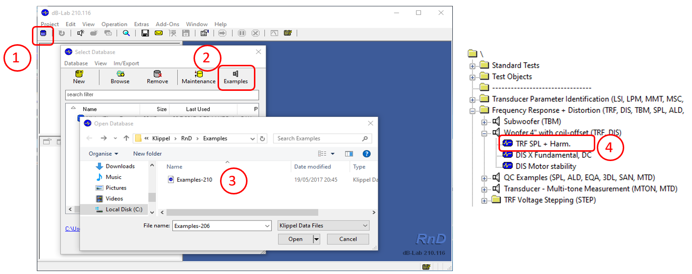
After double clicking on the operation TRF SPL + Harmonics the default result windows will be opened.

Stimulus Waveform#

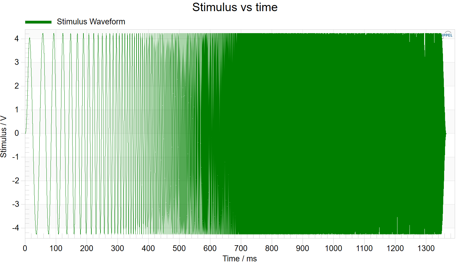
The time characteristic of the excitation signal, which is used to stimulate the system, reveals some fundamental properties of the transfer function measurement. The excitation signal is a sine wave that frequency varies continuously from the frequency F_min to the frequency F_max. At every discrete time step only one unique frequency is present. As frequency increases exponential with time (logarithmic sine sweep), each single frequency is mapped to one unique time step. This means that the linear time axis in the figure below could be replaced by a logarithmic frequency axis showing the instantaneous frequency of the sweep.

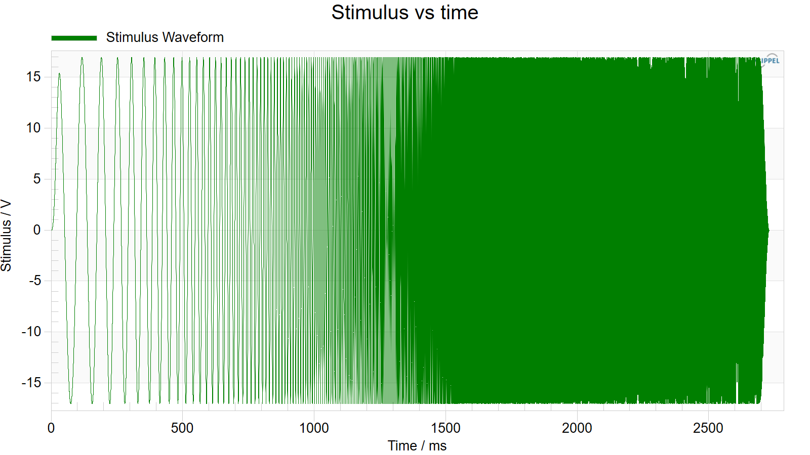
The main advantage of the log sweep is the ability to separate the linear response of the system from the nonlinear (harmonic) response. Intermodulation distortions are not excited as the stimulus contains one frequency at a particular time step.

Note

Müller, S. and Massarani, P. Transfer-Function Measurements with Sweeps J. Audio Eng. Soc., Vol. 49, No. 6, 2001 June.

First channel: Sound pressure response#

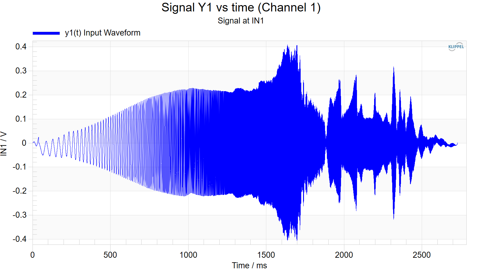
The TRF module is a 2-channel data acquisition system. Various input signals may be used to measure transfer functions such as external signal related to excitation signal but also external signal related to another external signal. In this example two external signals are recorded. The sound pressure level measured by a microphone is acquired on input channel Y1 and the displacement signal of the voice coil (measured by laser) is acquired on input channel Y2.

Due to the specific stimulus the envelope of the time domain signal of the transfer response is equivalent to the frequency response.

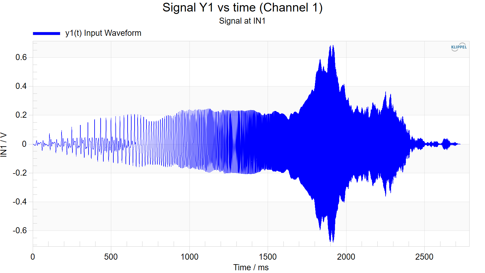
Time domain sound pressure response

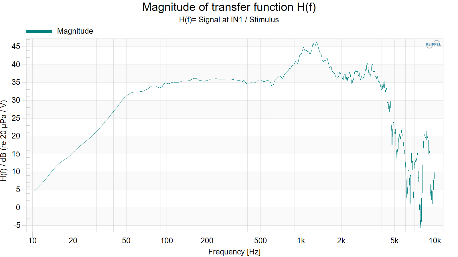Frequency domain sound pressure response

Please note the different scaling of the y-axis (linear in upper graph while log in lower graph).

Impulse Response#

The figure below shows the impulse response calculated from the sound pressure response.

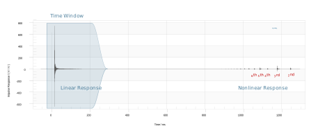
At the end of the time axis some minor artifacts can be noticed. These little peaks are the harmonic distortion information. Due to the very special excitation signal the individual harmonic distortion components are mapped to a narrow region of the time axis. This allows accurate separation of the linear and nonlinear responses as well as the extraction of the harmonic distortion for further analysis much faster as with stepped sine wave excitation technique.

Windowing#

The section of the impulse response that is used for further analysis can be selected (windowed) with two markers (e.g. to isolate direct radiation from early room reflections, diffuse field response and nonlinear artifacts etc.). On this way quasi-anechoic measurements can be performed. The part of the impulse response to be analyzed is marked by red color. Using the checkbox Set Window automatically, the position of the window can be either set automatically by the software or manually defined by user.

Note

The automatic window setting is only a rough estimation. Always check the position of the time window!

The easiest way to shift the markers is using the mouse for dragging. Alternatively, press SHIFT move the mouse to the desired marker position of the left marker and press the left mouse button. Press CTRL instead of SHIFT to move the right marker. If the position of the window is changed, all derived results will be recalculated without a new measurement.

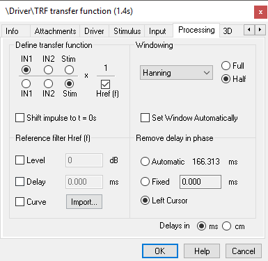
There are various applicable window shapes. Open the Processing Property Page and watch the Window setting. Half (typical used for driver measurements) and Full (for isolating harmonic distortion or room modes) shape is provided as well as various shape forms.

Fundamental + Harmonic Distortion#

This result window shows the fundamental and the harmonic distortion components of the sound pressure signal in absolute SPL. It is calculated using the current window setting (position and shape of selected window of impulse response).

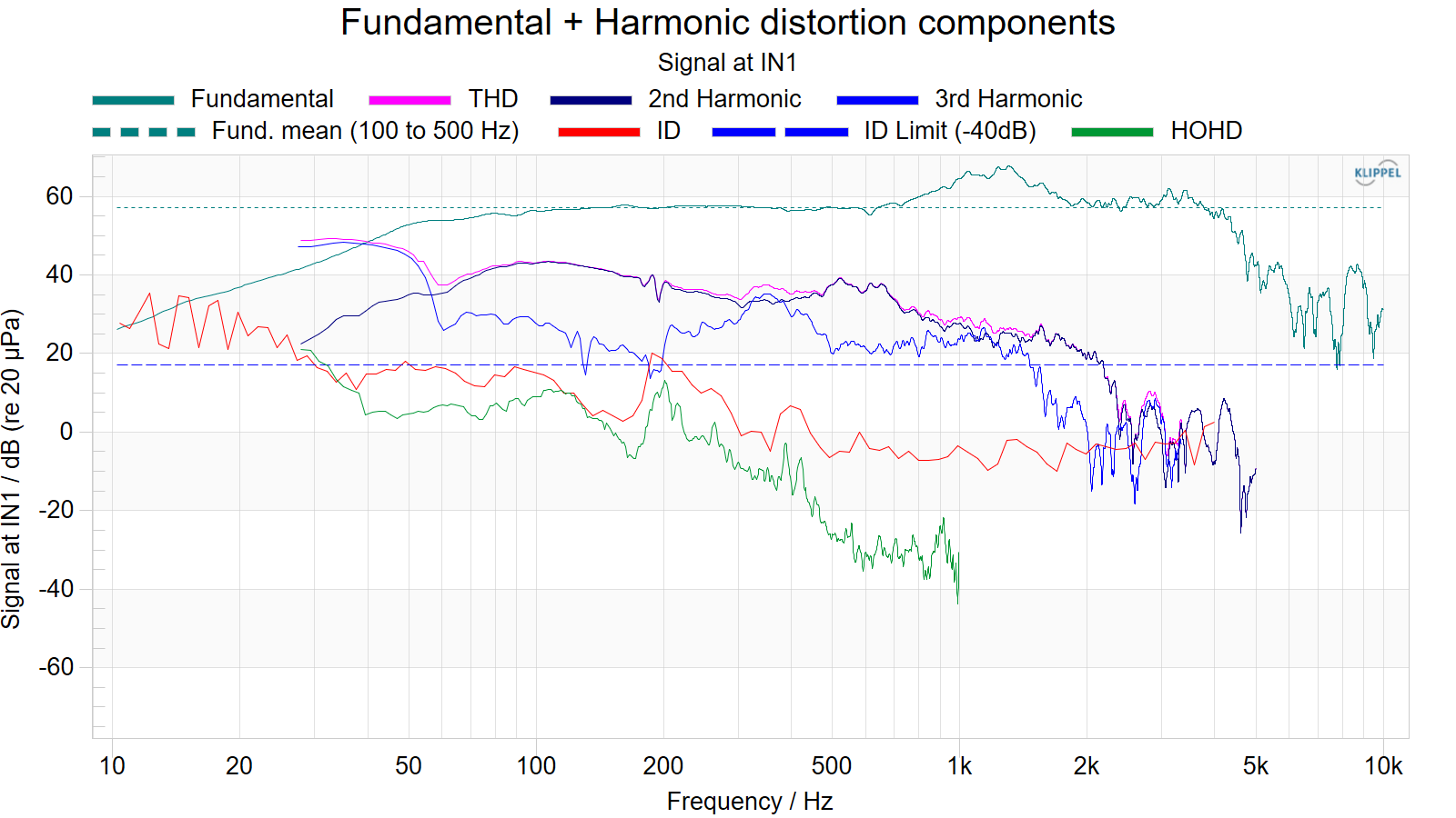
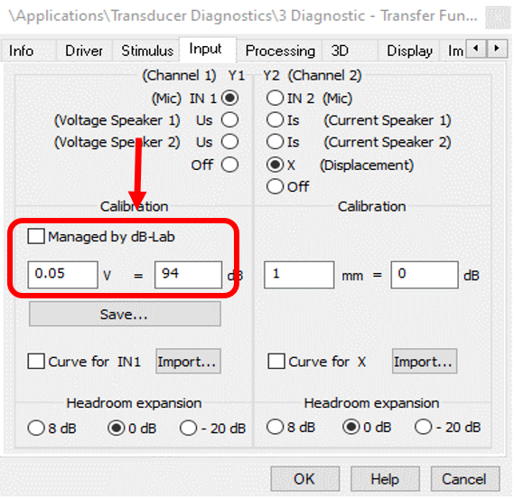
However the Fundamental is not divided by the stimulus thus meaning absolute SPL. To ensure that the absolute Sound pressure level is correctly calculated, make sure the microphone sensitivity is specified in the Input tab of the property page

See also

SPL Calibration

H(f) Magnitude#

The result windows H(f) Magnitude visualizes the transfer function, that means the sound pressure signal divided by the stimulus signal (in frequency domain). The result is a relative curve in dB independent on the magnitude of the excitation (holds valid for linear systems only).

Second Channel: Displacement#

Until now all results are discussed for the microphone input signal (routed to Y1, left side in property page input). Since the TRF is a two-channel system the second input signal Y2, recorded in parallel, may be investigated too. In the example a laser displacement sensor is routed to channel 2. Check the input property page for the current routing.

To view the results of the second channel select H(f) = X/Stim in the property page Processing.

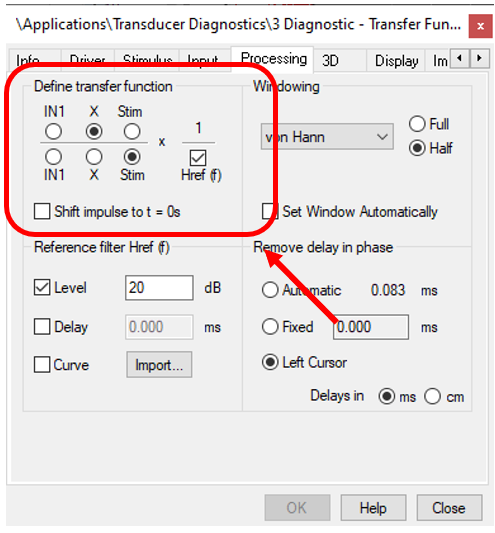
Pressing OK results in updated result windows. Watch now the results in the window H(f) Magnitude. The speaker clearly has a constant displacement below its resonance frequency f_s and a 12 dB roll-off above fs.

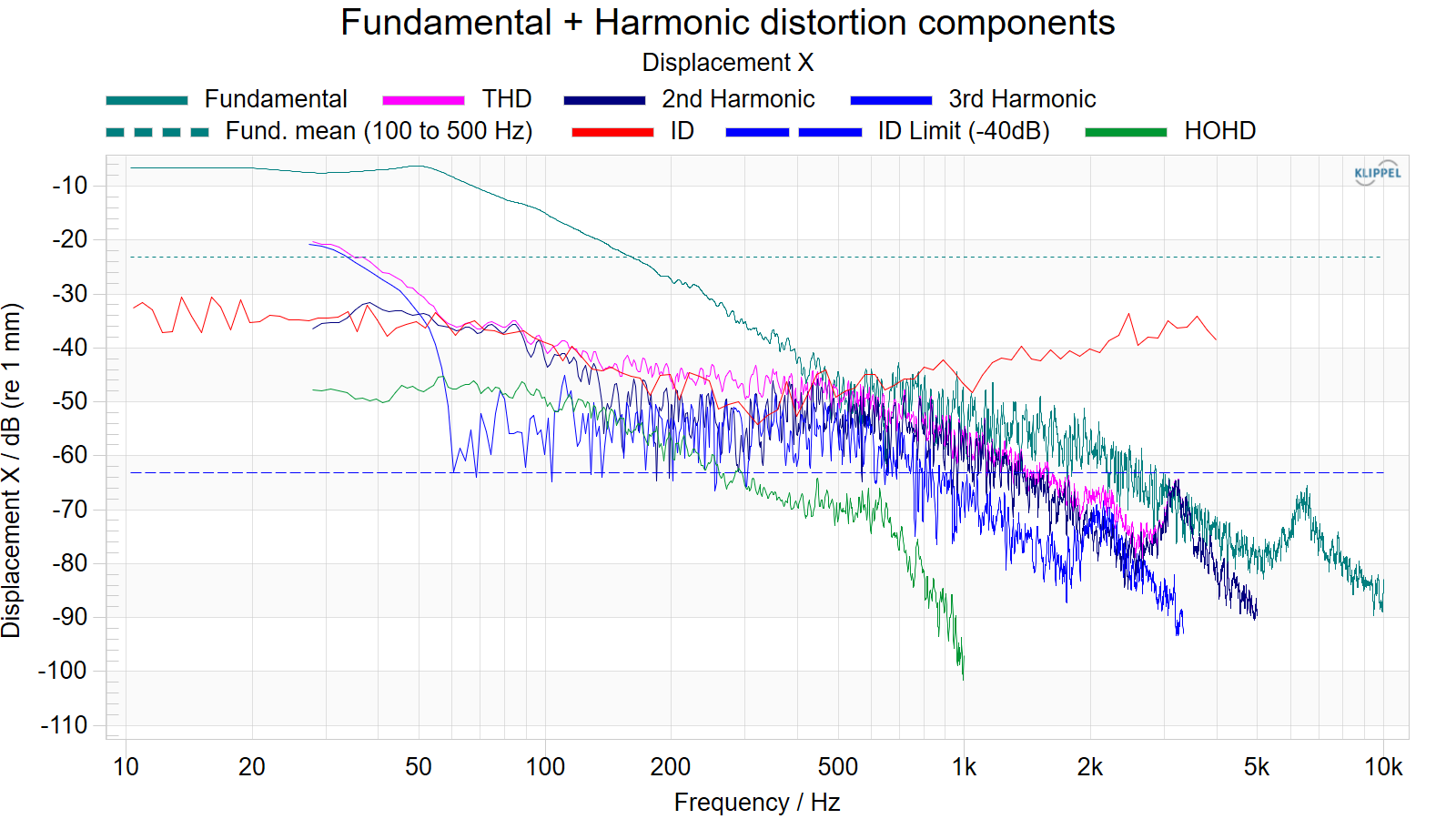
Open now the result window Fundamental + Harmonic Distortion. Now the harmonic distortion components are plotted. Note that at low frequencies where the driver has significant displacement the harmonic distortion are much higher than above 100 Hz. This nonlinear characteristic is measured very fast due the logarithmic sine sweep excitation.

Performing a new TRF (Part 2)#

In this part of the tutorial, you are guided to perform your first two measurements. As typical examples we will measure the SPL frequency response and the electrical impedance. Please follow the steps carefully and feel free to play with the set up afterwards.

SPL Measurement#

The following equipment is required:

Klippel Analyzer 3 or Distortion Analyzer (Power Monitor 8 Hardware does not support TRF measurements)
Microphone connected to input IN1 of the hardware unit
Driver mounted in laser stand
Power Amplifier

Hardware Setup#

Connect the Analyzer with the amplifier (Amplifier cable to connect OUT1 output with amplifier input and amplifier output with Amplifier input of the DA1). You will find more information in the chapter Hardware within the manual. Please note that this cable is not distributed by Klippel by default since the input connector of the Amplifier is not standardized.
Connect Analyzer with driver (use Speaker cable and connect Speaker 1 output with driver terminals)
Connect microphone signal output to IN1.
Connect Analyzer via USB to a Computer.
Connect power supply to Analyzer.
Switch hardware unit on

Create Operation#

It is recommended to use a new database. This leaves your example database unchanged.

Create a new database. Insert a new object and make a new TRF operation (Template #Default#). Detailed instructions are given in the dB-Lab manual section.

Now customize the setup for your first TRF measurement. Open the property page Info and Driver and fill in the required geometrical and nominal parameters as well as the additional information. These two pages are identical for all operations of the same object.

Measurement Setup#

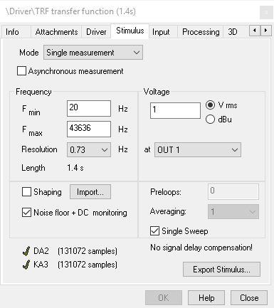
Open the property page Stimulus. Specify the frequency range, resolution, excitation level, number of averaging and the measurement mode.

The input routing is set in the page Input. Specify (Mic) IN1 for input channel Y1. Set Y2 to Off. You may enter the microphone sensitivity if known. Please refer to part 3 of the Tutorial on how to specify the microphone sensitivity. However, it is not required for this first measurement to know the exact sensitivity. You may use the default setting (this yields an incorrect SPL, but this does not matter for learning).

The Stimulus and Input property pages are measurement setup pages. That means that you will lose your data if you change setup parameters. This way any inconsistency between setup and data is avoided. The Processing, 3D, Display and I-Dist page contain post processing setup parameters. These values may be altered without losing data. The results are recalculated when new settings are confirmed with OK.

The Processing page determines the post processing of the data. The data windowing as well as the numerator and denominator of the transfer function are specified here. Use the default setting. Do not use any reference.

We do not use the 3D property page in this part of the Tutorial.

Start Measurement#

Make sure that the specified in property page Stimulus will not destroy your driver. Start the measurement after checking all connections by clicking on the start button .

Viewing results#

Open the default result windows by double clicking on the current TRF operation. Rearrange the result windows (horizontal tile) by selecting Window | Horizontal Tile in the menu or by clicking on the icon above the result window list.

Select the Impulse Response window and select the section of direct radiation with the two markers (several ways to position the markers are described in part 1 of the Tutorial). Make sure that the main impulse is within the window and that the peak of the main impulse is not attenuated too much.

Note

Normally the markers have to be placed in a very narrow section of the impulse response. This range depends on the geometry of your lab and on the distance between microphone and speaker. First place the marker roughly around the desired section of the impulse response. Press the F9 key to zoom between the markers and place the markers precisely.

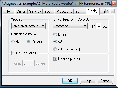
Open the result window Fundamental + Harmonic Distortion. The results are massively influenced by the setting of the property page Display. Set the values as shown below.

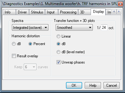
However, a variety of different options is available. Please take some time to explore the effect of different setting. Try at least the following options within the circled area:

No post processing / Averaged (1/3 oct) / Smoothed with some different bandwidth settings
dB / dB (level meter)

Using Template#

This measurement is quite standard and therefore the complete setup was entered manually instead of using some Operation Template. When creating new TRF operation some predefined setups may be selected. You can load the setting for the above example by choosing TRF SPL + harmonics operation Template. In the dB-Lab manual section the idea and the Handling of Operation templates is explained in detail.

Impedance Measurement#

The second example is the measurement of the electrical input impedance of a driver. This time we use a predefined template to load the complete setup.

The following equipment is required:

Klippel Analyzer 3 or Distortion Analyzer (Power Monitor 8 Hardware does not support TRF measurements)
Driver mounted in laser stand
Power Amplifier

Hardware Setup#

You may use the identical hardware setup as in the SPL example except the microphone. You don’t need any external sensor, because the analyzer has current and voltage sensors to measure the impedance.

Starting with the Distortion Analyzer (see label on back side) the unit has two different sensitivities for the speaker channels. The measurement of large signal parameter as well as the measurement of distortion require high voltage and current measurement capability. Contrary to this linear (small signal) measurements require a much more sensitive sensor characteristics to provide sufficient signal to noise ratio. Therefore the DA is equipped with a high power, low sensitivity sensor on Speaker Channel 1 and a low power, high sensitivity sensor on Speaker Channel 2. Each speaker channels Klippel Analyzer 3 supports both, low and high sensitivity. This can be configured in the KA3 signal configuration. For more details please see the hardware manual.

Note

For linear measurements (such as LPM and TRF) is strongly recommended setting using a high sensitivity channel

Create Operation#

Use the database you created above and insert a new TRF operation. Use the Operation Template TRF impedance when inserting the operation. Enter a new name for the inserted operation. Detailed instructions on templates are given in the dB-Lab manual section.

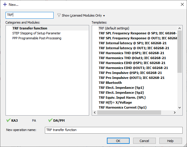
The operation template is described in the Comment field of the Info property page. You can read the comment after inserting the operation. Please refer to this field if the template name gives not sufficient explanation.

Measurement Setup#

Please check the setup configuration from the template. The impedance will be measure from 1 Hz up to 20 kHz using Speaker Channel 2. Electrical measurements will be falsified by windowing. Therefore the window shape is set to Rectangular and the whole impulse response is selected for analysis (check the marker positions in result window Impulse Response; the markers will be displayed in the impulse response window).

Result windows#

Open the result window H(f) Magnitude. It shows the magnitude of the impedance in Ohm. The result window H(f) Phase shows the phase response. Please note, that no small signal (linear) parameters are derived from the impedance by the TRF software. To determine the Thiele-Small parameters, use the LPM – Linear Parameter Measurement module.

Property page Display#

Since the magnitude of the impedance has a linear scale, Absolute is selected in the section Transfer function. For impedance measurements it is recommended to apply some smoothing (e.g. with a bandwidth of 1/24 octave). The spectral lines are very dense at higher frequencies (the number of lines increases for a constant relative bandwidth due to the equidistant spacing of the spectral lines), in fact far too dense to be displayed. This property can however be utilized to attenuate higher frequency noise by averaging over neighboring spectral lines (smoothing).

Customizing TRF (Part 3)#

In this part of the tutorial various advanced aspects are discussed to use more powerful features and improve the performance of the TRF measurement.

You should read this part of the Tutorial if you are familiar with the basic functionality of dB-Lab and of the TRF operation (Tutorial Part 1 and 2).

SPL Calibration#

This section describes how to calibrate the TRF module for acoustical measurements. The microphone sensors including sensitivity are centralized managed by dB-Lab for all measurement module since version 212. For further information, about the general sensor calibration, please see the KLIPPEL Analyzer Hardware section Sensor Handling.

However the TRF module can be used for the sensor calibration directly, which is described in the following.

Using a Pistonphone#

If a pistonphone (or calibrator) is available, an automatic procedure may be used to determine the sensitivity of the microphone. The calibration can be done with different pistonphones and different frequencies (e.g. 250 Hz or 1 kHz). To perform this procedure open the property page Stimulus

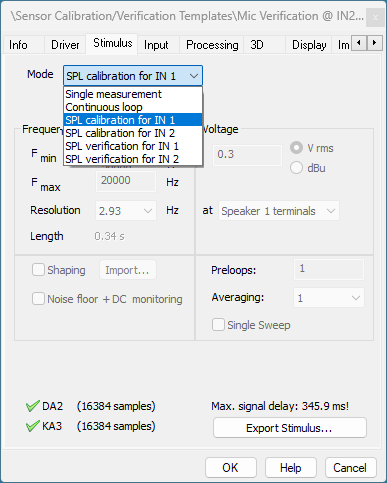
and select the SPL calibration for IN1 mode. There is also an option for calibrating input channel 2.

Do the following steps:

Connect the output of the microphone preamp with connector IN 1
Connect the pistonphone with the microphone
Start the SPL calibration mode by clicking .
Enter the SPL produced by the pistonphone.
Put the pistonphone into operation and click OK.
You will get a message if the SPL calibration was successful. The calibration routine will set the according calibration parameters for IN 1 in property page Input. If the SPL calibration failed check the result windows Y1(t) and Y1 (f) Input Spectrum and go back to step 3 after you have checked the hardware connections.
Once the calibration is finished you can store the calibration data as a sensor file.
To use your saved sensor file, select the sensor for the corresponding input channel. Refer to Adding and Selecting Sensors for more information.

Manual Definition of Sensitivity#

If the dB-Lab sensor management is turned off, the sensitivity can be also specified directly for a TRF operation. Open property page Input, select (Mic) IN 1 or IN 2 (Mic) enter the sensitivity in group Calibration (for instance 0.0134 V = 94 dB for a sensitivity of 13.4 mV/Pa). Note that 1 Pa equals approximately 94 dB.

How to load a Microphone Correction Curve?#

The normalized microphones frequency response, as it is typically provided by the microphone manufacturer or calibration laboratory, could be used as a microphone correction curve. The measured input spectrum will be divided by the microphone correction curve to compensate for its frequency response. Thus, the correction curve is subtracted from the measured response curve in dB.

The correction curve may be specified

as magnitude curve versus frequency in dB or
as magnitude (in dB) and phase (in degree) curve versus frequency.
it must be normalized at the frequency the sensitivity was specified (typically 250 or 1000 Hz).

To load a microphone correction curve do the following steps:

Open property page Input. Select (Mic) IN1 if you want to connect the microphone to input IN 1 (alternatively select (Mic) IN2 if the microphone is connected to IN 2).
Click on the Import… button in the corresponding group Calibration. This will open a dialog where you can import the microphone correction curve. Click Load… in order to load the file with the correction curve (see section Curve import and export in the TRF Reference for further information about the required format).
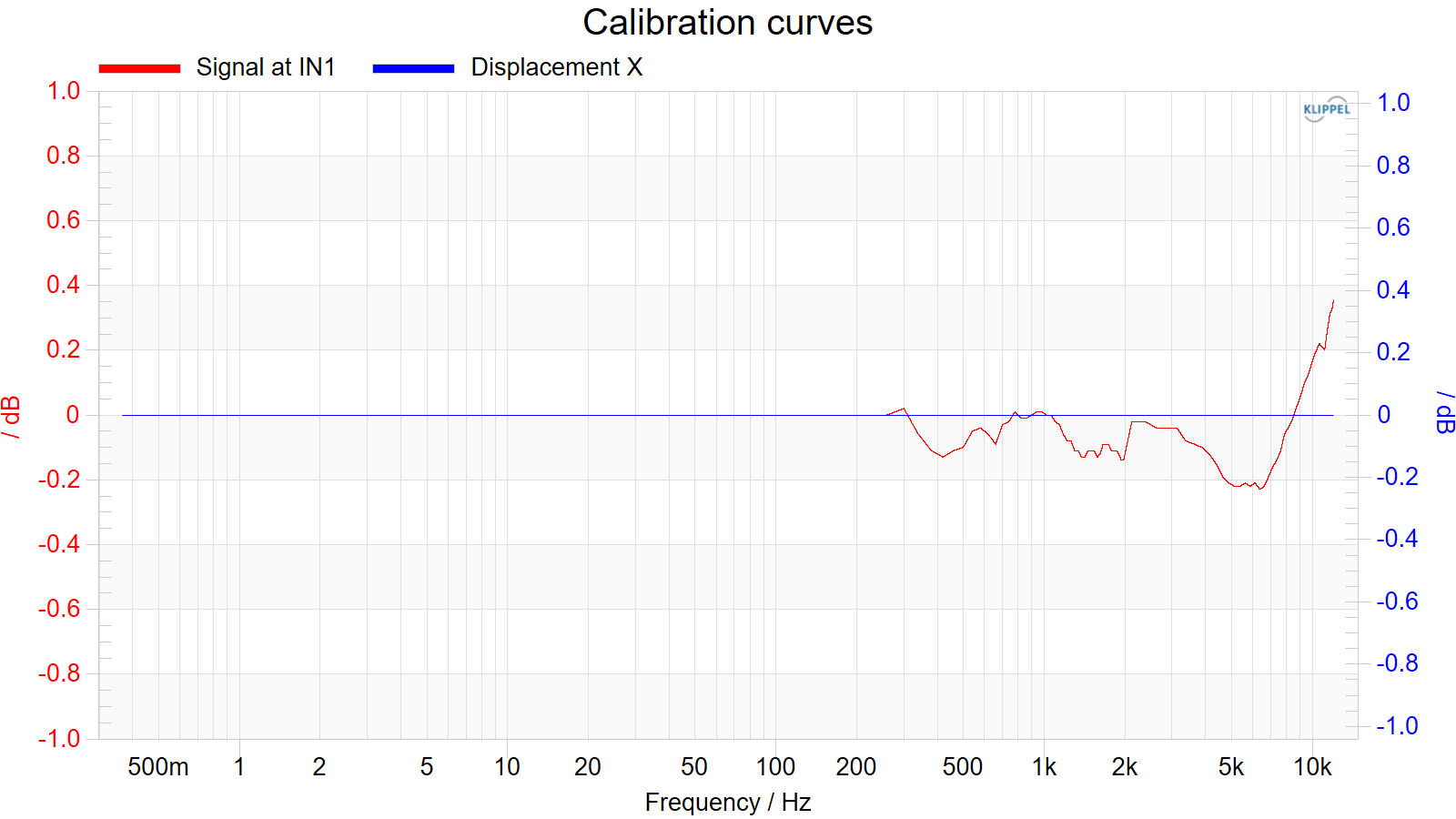
Check the proper import and activation of the correction curve in result window Calibration Curves. The window shows the correction curves actually used for the measurement.

Note

The calibration curve are displayed for the frequency range only specified in property page Stimulus. For each spectral line of measured signal a correction value is calculated by linear interpolation. Select Mark Data Points in the context menu of the result window Calibration Curves to view the individual points.

Export Transfer Function Data#

The export of transfer function data to post processing tools such as simulation software is essential for a seamless design cycle.

The transfer function data is exported to the clipboard in a three-column format (see section Curve import and export in the Reference). The first column contains the frequency in Hz. The second and the third column list the magnitude (in dB or real physical unit) and the phase in degree.

Note

The unit for the magnitude column is controlled by the unit combo box in group Transfer function in property page Display. The magnitude is exported in physical units (like V, A, V/V, etc.) if Absolute is selected. For the options dB and dB (level meter) the magnitude is exported in dB. The unit for the phase column is always degree.

There are several options for the transfer function export. The user can export either the

Magnitude of the true transfer function H(f) (result window H(f) Magnitude) or the
Magnitude of the Fundamental of the numerator signal (result window Fundamental + Harmonic Distortion).

The magnitudes can be combined with the

Total phase (result window H(f) Phase), the
Minimal phase (result window H(f) Minimal Phase) and the
Excess phase (result window H(f) Excess Phase).

The number frequency points of the transfer function points can be log-reduced. For some simulation software only a view hundred (logarithmically spaced) points are needed. The user can specify the desired number of frequency points per octave. If the checkbox Log-reduce is activated only the specified number of points (picked logarithmically) will be exported.

Note

When using the logarithmic reduced export make sure that the applied Smoothing in the Display Tab is similar to the export resolution.

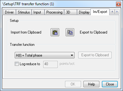
To export the transfer function data to the clipboard open the property page Im/Export and click the button Export to Clipboard. The button will be disabled if no transfer function data is available. The button will be enabled as soon as the transfer function is calculated.

Open the clipboard editor (double click icon in the right part of the status bar). Click Save… in order to save the data in a plain text file.

Result Overlay#

TRF “Result Overlay” feature was removed for 212.800 and later due to problematic conflicts with other features.

Modes of Operation#

Four different Mode may be selected in the Input page:

Single measurement

Default setting. A single measurement will be performed and the results stored in the database.

Continuous loop

This setting allows repetitive measurements without starting each measurement individually. The loop is started by clicking on the icon. The loop may be terminated by clicking on the icon. This way the loop is paused after the measurement has finished. Clicking on the icon stores the results of the last measurement in the database. If you use the icon during a measurement the data will be discarded.

Options: The parameter Time between measurements specifies the time between the individual measurements. Please note that this time should be sufficient for calculating and updating the open result windows. If not, blank result windows will occur.

SPL calibration for IN1

Mode for calibrating the first input channel for acoustical measurements. See section SPL Calibration

SPL calibration for IN2

Mode for calibrating the second input channel for acoustical measurements. See section SPL Calibration

See also

SPL Calibration

Using References / Comparing results#

It is very easy within the TRF module to use reference curves e.g. for comparing results and determining deviations between measurements.

Let’s assume that you want to know the deviation the 30° off axis response from the on axis response.

Create a new TRF operation. Enter a setup according to your needs. You can speed up this process considerably if you use a template.
Measure the on axis response.
Create a second TRF operation with identical setup. Use the according template or export and import the setup via the clipboard (property page Im/Export).
Export the transfer function data of the first TRF to clipboard. Click on the Export to clipboard button in page Im/Export. Alternatively copy the Magnitude curve from result window H(f) Magnitude to the clipboard (mark the curve by clicking on the curve label and select Copy Curve in the context menu). Note that no phase information will be exported in this case.
Open property page Processing of the second TRF, click on the Import… button in group Reference. This will open a dialog for importing the reference curve. Click Paste to import the curve from the clipboard. Note that the reference curve will only be used if this check box is selected.
Open the result window Reference Curve and check the correct import of the reference curve.
Adjust your microphone to a 30° position. Measure the off axis response.
Open property page Display and select dB or dB (level meter). The result window H(f) Magnitude shows now the deviation of the 30° off axis response from the on axis response in dB.

How to View Higher Order Harmonics?#

The TRF module measures the harmonic distortion components up to the 24^th order. For clarity reasons only the 2^nd and 3^rd harmonics are displayed by default. If you want to view the higher order harmonics, right click and select Customization Dialog… | Subsets from the popup menu. Select the harmonics you are interested in and click OK.

How to Speed up Marker Placement?#

Normally the markers have to be placed in a very narrow section of the impulse response. This range depends on the geometry of you lab and on the distance between microphone and speaker. First place the marker roughly around the desired section of the impulse response. Press the F9 key to zoom between the markers and place the markers precisely.

How to measure instantaneous distortion?#

Instantaneous distortion can be measured with the TRF Pro Module. For detailed information about the measurement procedure see application notes:

TRF Reference#

Overview#

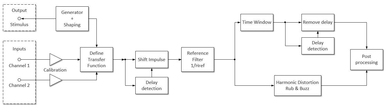
The TRF module is aimed at transfer function measurements. The system under test is excited by a (continuous) sine sweep. Two system responses up to 128k can be acquired simultaneously at sample rates up to 96 kHz. The two responses can be acoustical responses, the voltage or current signal at speaker terminals (using the internal sensors of the Analyzer hardware) or the diaphragm displacement (using the laser sensor). After the measurement several transfer functions can be calculated by post-processing (response1/stimulus, response2/stimulus, response1/response2 and the corresponding reciprocal). First the TRF module calculates the impulse response. Using two markers the user can select the range of the impulse response that contains direct radiation only. As only that range is used for further calculations, room reflections are excluded and a quasi-anechoic measurement is provided. Furthermore the TRF module extracts the harmonic distortion components (versus frequency) from the measured impulse response. They are displayed in the same plot as the fundamental (magnitude of transfer function) as well as in an extra plot as percent or dB ratios referred to the fundamental. Additionally the delay time, minimum phase, total delay, excess delay, the spectral cumulative decay (CSD), the Wigner distribution and a Spectrogram are calculated.

Property pages#

STIMULUS Page#

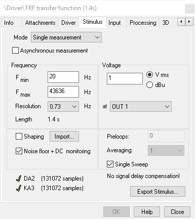
Frequency#

Minimal frequency: \(F_{\text{min}}\) in \(\text{Hz}\)

Minimal frequency to be analyzed. It determines the start frequency of the stimulus sweep.

\(F_{\text{min}}\) must be greater than \(0\text{Hz}\)
Maximal frequency: \(F_{\text{max}}\) in \(\text{Hz}\)

Maximal frequency to be analyzed. It determines the end frequency of the stimulus sweep.
Resolution: Desired resolution for analysis. Determines the duration of the sweep.

The time below in brackets (\(1.4s\) in the figure above) is the duration of the sweep.
FFT Size: FFT Size is dependent on \(F_{\text{max}}\) , the Resolution and the measurement device.

The number of samples is shown in the left bottom corner of the Stimulus Page.

Shaping#

Clicking the Import… button opens a dialog where a curve can be imported (see section Curve import and export in the Reference). The stimulus spectrum is shaped according to that curve after activating the checkbox Shaping. The stimulus shaping curve must be given in dB. The shape of the stimulus spectrum is adjusted to the shape of the imported curve (check result window Stimulus Spectrum). For security reasons the shaping curve is automatically scaled before applying it to the stimulus. The scaling limits the maximal shaping factor to 0 dB, i.e. the stimulus amplitude will never be increased. The shape of the spectrum determines the crest factor of the waveform. The default shape of the stimulus spectrum yields to the optimal crest factor of 3 dB.

Voltage#

RMS voltage of the stimulus (RMS amplitude of the sweep sine signal). The voltage can be specified in either \(V_{\text{RMS}}\) or in \(\text{dBu}\). Check result window Stimulus (t) before you start measurement. It shows the waveform of the excitation signal that is applied to the measurement

If at Speaker 1 terminals is selected the specified stimulus voltage is the voltage at the terminals of the speaker connected to the Speaker 1 output. The amplifier input can be either connected to the OUT 1 or OUT2 output. The gain of the amplifier is measured at 750 Hz without load prior to the main measurement and the excitation level is adjusted accordingly. If the measurement is repeated with the same setup parameters the amplifier gain is not measured again in order to allow fast measurement repetitions. Therefore the amplifier gain must not be changed during a measurement session.

Note

The voltage applied to the speaker terminals will usually be slightly smaller than the specified one. This is because the amplifier gain decreases if a load is connected.

If at Speaker 2 terminals is selected the speaker must be connected to the Speaker 2 output and the amplifier input to the OUT1 or OUT2 output.

If at OUT 1 or at OUT 2 is selected the specified stimulus voltage is the voltage at the output connector OUT 1 or OUT 2 respectively. At OUT 1 will switch on the Speaker 1 relays, at OUT 2 will switch on the Speaker 2 relays, independent from the input channel selection.

Note

If an amplifier is used and at OUT 1 or at OUT 2 is selected the specified stimulus voltage is the voltage at the amplifier input. The level of the amplifier output signal can be considerably higher than the specified level and can possibly destroy your speaker! Please make sure that no amplifier is connected if you use at OUT 1 or at OUT 2.

Noise floor + dc monitoring#

If selected, a noise floor measurement is performed before the main measurement. This measurement allows furthermore determining offset factors which are important for the correct measurement of the dc components of the measured signals. Therefore the dc components are shown in Table Results + Settings only if the checkbox is selected. You will see the measured noise floor in the result windows Y1(f) Input Spectrum and Y2(f) Input Spectrum as black lines together with the red and blue signal lines obtained during the main measurement.

Preloops#

Number of stimulus repetitions before the actual measurement. At least one preloop is essential to compensate effects due to time delays.

Averaging#

Number of measurement repetitions for noise floor reduction.

Single Sweep#

If Single Sweep is activated no Preloop is executed and no Averaging is applied. In this configuration, longer time delays cannot be compensated, because the recording of the response is synchronized with the playback of the stimulus. The end of the sweep wouldn’t be recorded. For measurements with short time delay (e.g. passive speakers in the near field) this setting can be used, because stimulus has a short fade-in and fade-out time that can compensate minor delays. The maximum allowed signal delay is displayed in right bottom corner of the Stimulus page.

Asynchronous measurement#

Special measurement mode to measure wireless devices (e.g. Bluetooth®, Wi=Fi etc.) and devices in open loop with an asynchronous playback by an external player.

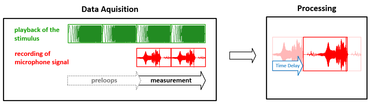
If the Asynchronous mode is activated, the stimulus is played twice and the TRF automatically detects the time delay picks the best part of the recorded signal to avoid artefact from clock jittering. By using preloops, the asynchronous measurement mode also compensates for long time delays.

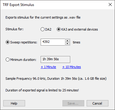
Export Stimulus#

To measure devices in open loop the stimulus can be exported as wav-file. The exported wav-file can be played on device as loop and the TRF is capturing the response asynchronous.

Device Measurement Capabilities#

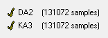
On the bottom of the Property Page are two indicators displaying the possibility of measuring with the configured stimulus with either the DA2 or the KA3. If the symbol next to the device is a green tick, the measurement is executable. If the symbol is a red cross the device is not able to execute the measurement. For more information about the reason click on the device name.

INPUT Page#

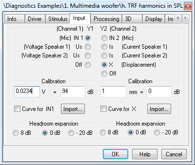
Y1 (Channel 1)#

Signal that is acquired on channel 1. IN 1 is the signal at the IN 1 connector of the Distortion Analyzer (usually a microphone). \(U_s\) is the voltage at the terminals of the speaker connected to the output Speaker 1 or Speaker 2 respectively. If you choose Off, no signal is acquired on channel 1. That way the measurement can be speeded up.

Y2 (Channel 2)#

Signal that is acquired on channel 2. IN 2 is the signal at the IN 2 connector of the Distortion Analyzer (usually a microphone). Is the current at the terminals of the speaker connected to the output Speaker 1 or Speaker 2 respectively. X denotes the signal from the laser displacement sensor. If you choose Off, no signal is acquired on channel 2. That way the measurement can be speeded up.

Calibration#

Conversion from physical units to dB for the signals Y1 and Y2 acquired on channel 1 and channel 2 respectively. The user can specify how many volts (or amperes, millimeters respectively) correspond to how many dB. This provides a convenient way to calibrate the TRF e.g. for acoustical measurements (section SPL Calibration in part 3 of the Tutorial). The spectra of Y1, Y2 and the transfer function are plotted in dB and the plots are scaled according to the specified dB conversion.

A calibration curve for the corresponding signal can be loaded by clicking on the Import… (see section How to load a Microphone Correction Curve?). For each sensor signal (IN1, IN2, \(U_s\), \(I_s\), X) a separate calibration curve can be imported and stored in the database. The measured spectra \(Y1(f)\), \(Y2(f)\) are divided by the calibration curve for all signal lines

\[Y_{\text{cal}}(f) = \frac{Y(f)}{\text{Calcurve}(f)}\]

If the adjoined check box is selected. If the check box is not selected, the measured signal is left unchanged. The calibration curve is used to compensate frequency dependency of the hardware. This way the frequency dependency of a microphone can be eliminated for instance. Microphone manufacturers usually provide sensitivity curves that show this frequency dependency. These curves don’t have to be inverted and can be directly loaded into the TRF by clicking on Import… and then on Load…. Furthermore the whole signal path can be included in the compensation. For instance to compensate the current measurement replace the driver by a calibrated resistor. The measured current spectrum \(I_s(f)\) can then be used to generate a calibration curve.

Headroom expansion#

The headroom for data acquisition can be increased by 8 dB to cope with very large signals that exceed the normal operational range. To increase the measurement accuracy for very small signals the headroom can be decreased by 20 dB as well.

PROCESSING Page#

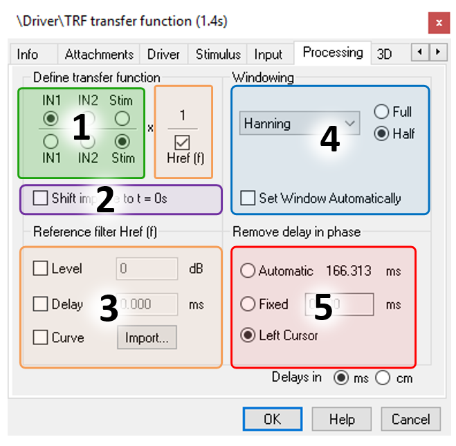
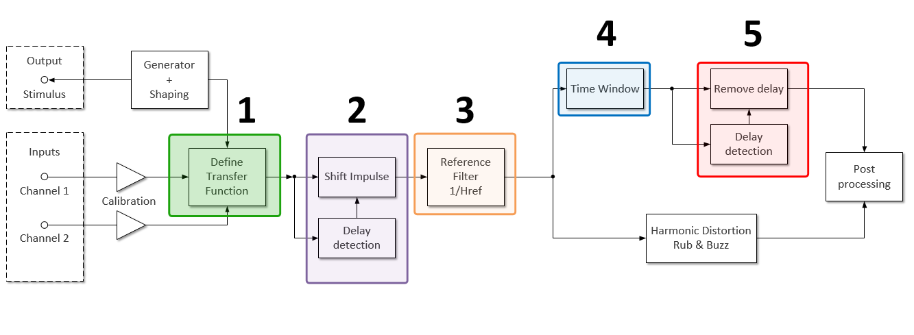
Define transfer function#

Here the nominator and denominator of the transfer function \(H(f)\) have to be selected.

Shift impulse to t = 0s#

When measuring wireless audio devices the delay e.g. of a Bluetooth® transmission is varying. By activating this checkbox the delay of the measured Impulse Response is automatically detected and removed from the impulse response. That means the main impulse is always shifted to t=0s and a manual time window to remove reflections can be defined.

Reference filter#

The user can specify a scalar reference value (in dB) and a reference curve. If the check box Level is selected the transfer function is divided by the reference value. This means that if the reference value is e.g. 5 dB and the transfer function is plotted in dB, it will be shifted down by 5 dB.

In addition a delay in ms can be added or removed by using the check box Delay.

Clicking on the Import… button opens a dialog where a reference curve can be imported (see section Using References / Comparing results). There are two formats supported. The first format is a two-column matrix where the first column gives the frequency in Hz and the second the reference in dB. Furthermore a three-column matrix is supported where the first column contains the frequency in Hz the second the magnitude of the reference in dB and the third the phase in degree. The transfer function \(H(f)\) is divided by the reference if the adjoined check box is selected. This way the user may refer the actual measurement to some reference measurement. Furthermore known disturbances (e.g. due to the room) can be compensated.

Windowing#

Several data windows can be applied to the selected range of the impulse response (Rectangular, Cosine, Hanning, Hamming, Blackman and the Kaiser window). To select the direct sound range of the impulse response set the two markers in the result window Impulse Response, Energy-Time Curve and Step Response. Use the mouse to drag the markers. Alternatively, press SHIFT, move the mouse to the desired marker position of the left marker and press the left mouse button. Press CTRL instead of SHIFT to move the right marker. To zoom between the markers press F9.

If Full is selected a symmetric window is used and the window summit is centered between the markers. Therefore the peak of the impulse response should be halfway between the two markers. If Half is selected, only the right half of a symmetric data window is used. The window has its summit at the left marker and its minimum at the right marker. Therefore the left marker should be placed very close to (but left of) the peak of the impulse response. For acoustical measurement, Half is normally the right choice. For illustration toggle between Full and Half and check the effect that is has on the windowed impulse response in result window Impulse Response.

Note

The automatic window setting is only a rough estimation. Always check the position of the time window in the impulse response window!

Remove Time Delay in phase#

The time delay can be detected automatically by the software (Auto) or specified manually by the user (Fixed). If Fixed is selected, this time delay will be used for the calculations instead of the measured one.

The automatic time delay detection first removes the minimal phase (calculated with the Hilbert transformation) from the measured total phase. Then the impulse response is calculated that corresponds to the so obtained “excess” phase. The time delay is the point where the envelope of this impulse response reaches its maximum.

The unit for the time delay can be toggled between milliseconds (ms) or centimeter (cm). If cm is selected, the time delay is converted to the corresponding distance = time delay sonic speed.

3D Page#

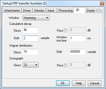
Window#

Data window for the calculation of the cumulative spectral decay plot (CSD), the Wigner distribution and the Spectrogram.

Cumulative decay#

Slices: Number of time slices for the cumulative spectral decay plot
Shift: Spacing of (distance between) the time slices
Window rise time: Rise time (from 10 % to 90 %) of the data window used for calculating the cumulative spectral decay plot. Short rise times improve the time resolution but decrease frequency resolution, and vice versa.
Floor: Floor value of the plot. If the adjoined check box is selected the specified floor value will be used, otherwise the floor value will be determined automatically.

The cumulative spectral decay plot shows the decay of the individual frequency components after a sinusoidal excitation is suddenly switched off.

The first time slice of the CSD is calculated using the entire (direct sound) impulse response specified with the two markers in result window Impulse Response. The following time slices are calculated using reduced versions of the direct sound impulse response. For this the impulse response is windowed with an additional window for which the user can select shape and rise time at property page 3D. The window start time is successively increased

\[t_{\text{start}} = t_{\text{left marker}}+ n \text{ Shift}\]

where \(n = 1, 2, …\), Slices denotes the index of the “time slice”. The window end time is fixed at the position of the right marker. This way the reduced impulse responses contain less and less information about the beginning of the response.

The cumulative spectral decay consists of the FFTs of the reduced impulse responses. The individual slices reveal the frequency contents that is present in the system after \(n \text{ Shift}\) ms.

Wigner distribution#

Slices Number of time slices for the Wigner distribution Shift Spacing of (distance between) the time slices

The Wigner distribution shows the energy present in the direct sound response (specified with the two markers in result window Impulse Response) versus frequency and time.

Spectrogram#

Slices: Number of time slices for the Spectrogram. According to the number of time slices the direct sound response (specified with the two markers in result window Impulse Response) is divided in overlapping sections for which short time FFTs are performed.
FFT: Corresponding size of the short time FFTs. The size depends on the parameter Slices and the distance between the markers in result window Impulse Response.
Floor: Floor value of the plot. If the adjoined check box is selected the specified floor value will be used, otherwise the floor value will be determined automatically.

DISPLAY Page#

Spectra#

Display mode for the result windows Y1(f) Input Spectrum and Y2(f) Input Spectrum. No post processing shows the signal lines (red or blue), and the noise floor lines (black) if the option Noise floor was selected in property page Stimulus. In the modes Integrated (1/3 oct.) and Integrated (octave) the square root of the signal lines energy is shown for IEC standard 1/3 octave and octave bins respectively.

Harmonic distortion#

Determines the unit for the relative harmonic distortion in result window Harmonic Distortion. If Percent is selected the distortion measures are plotted in percent. The second option will give the distortion measures in dB (100 % corresponding to 0 dB).

Transfer function + 3D plots#

Display mode for the result windows H(f) Magnitude, Fundamental + Harmonic Distortion, the phase, group delay and the 3D result windows (Cumulative Spectral Decay, Wigner Distribution and Spectrogram).

The combo box select averaging and smoothing:

No post processing shows the results without any post processing.
In the modes Averaged (1/3 oct.) and Averaged (octave) the average of the fundamental and the harmonics is shown for IEC standard 1/3 octave and octave bins respectively. The band average values are calculated according to IEC 60268-21 by:

\[{\widetilde{p}}_{m} = \left[ \frac{1}{K} \sum_{k=1}^{K} (\widetilde{p}_k)^2 \right]^{\frac{1}{2}}\]

The Averaged options do not apply to the phase, group delay and 3D result windows.
Smoothed shows the transfer function and 3D results smoothed over the specified octave ratio. Phases will only be smoothed if Phases: Unwrapped is selected.

The radio buttons control scaling for H(f) Magnitude, Fundamental + Harmonic Distortion and the 3D result windows (windows Cumulative Decay, Wigner distribution and Spectrogram).

Linear uses physical units on a linear scale a linear Y scale with the unit depending on the input channel
If dB is selected, the curves are plotted in dB.

This option does not apply to the Wigner distribution as this distribution can have negative values.
dB (level meter) plots the curves in dB, imitating the plots produced by the classical level meters of the old days. It uses a fixed frequency axis that stretches from 10 Hz to 40 kHz while the range of the y-axis is fixed to 50 dB. This option only applies to the result windows H(f) Magnitude and *Fundamental + Harmonic Distortion

Unwrap phases#

If selected the phases in the result windows H(f) Phase, H(f) Minimal Phase and H(f) Excess Phase will be displayed unwrapped.

IM/EXPORT Page#

Setup#

Import from Clipboard: Imports all TRF setup parameters from the clipboard.

Export to Clipboard: Exports all TRF setup parameters to the clipboard.

Transfer function#

Export to Clipboard: Exports either the transfer function or impulse response to the clipboard in a desired format. The following options are available:

H(f) + Total Phase
H(f) + Minimal Phase
H(f) + Excess Phase
Fundamental + Total Phase
Fundamental + Minimal Phase
Fundamental + Excess Phase
Windowed Impulse Response
Measured Impulse Response

All transfer functions are exported to the clipboard in a three=column format (see section Curve import and export in the Reference). The first column contains the frequency in Hz. The second and the third column list the magnitude (in dB or real physical unit) and the phase in degree. The unit for the magnitude column is controlled by the unit combo box in group Transfer function in property page Display. There are several options for the transfer function export. The user can export either the magnitude of the true transfer function \(H(f)\) (result window H(f) Magnitude) or the magnitude of the Fundamental (result window Fundamental + Harmonic Distortion). The magnitudes can be combined with the total phase (result window H(f) Phase), the minimal phase (result window H(f) Minimal Phase) and the excess phase (result window H(f) Excess Phase).

The number frequency points of the transfer function points can be log-reduced. For some simulation software only a view hundred (logarithmically spaced) points are needed. The user can specify the desired number of frequency points per octave. If the checkbox Log-reduce is activated only the specified number of points (picked logarithmically) will be exported.

Note

When using the logarithmic reduced export make sure that the applied Smoothing in the Display Tab is similar to the export resolution.

For exporting the impulse response \(H(t)\), the TRF provides two options. Export with and without windowing. The exported impulse response is normalized and has a natural scaling. This is useful, because the length of the stimulus has a significant influence on the level. To get the original level from the measurement, the data has to be divided by the sampling freuency.

Note

The section Remove delay in phase on property page processing has no influence on the exported impulse response.

See also

Export Transfer Function Data

I-DIST Page#

(TRF Pro only)

In this page the settings for the instantaneous distortion measurement are selected.

Mode#

This combo box controls the mode of the instantaneous distortion measurement.

ParameterName

Impulsive Distortion: This mode can be used to measure impulsive distortion according to IEC60268-21 and rub & buzz symptoms. By the chosen harmonic distortion order of 10^th or 20^th the fundamental and lower order harmonic distortion are removed from the measured signal and the impulsive high frequency components will be isolated and considered for the calculation of the impulsive distortion measures. All low frequency component and reverberant sound would be removed as well.
Rub & Buzz: This mode is used for rub & buzz detection if no “golden unit” is available. rub & buzz distortion typically produce symptoms in the full frequency band, harmonic and non-harmonic. Those distortion may be masked by lower order regular speaker distortion, which are filtered out by tracking high pass filters of selectable order between 10^th and 20^th order. In difference to the Impulsive Distortion, the Rub & Buzz mode includes also low frequency components that could be used to detect sub harmonics or other artefacts in the signal. However this mode needs a good acoustic environment, because reverberant sound will appear in the residual signal response and may affect the impulsive distortion measures.
THD + Rub & Buzz: In this mode any behavior that deviates from linear behavior is measured. Both the regular driver distortions (due to motor and suspension nonlinearities, etc.) and impulse distortions (rub & buzz) are included. This is useful to identify any nonlinear effect of the driver. No “golden unit” is needed.

Note

In dB-Lab vesions 210.826 and lower this mode is called “All Distortion”
Deviation all distortion: In this mode a “golden unit” is needed. The golden unit is used to remove the unavoidable regular driver distortions (due to motor and suspension nonlinearities, etc.) from the measurement. For this the golden unit has to be measured first. After the measurement has finished click the Learn button to identify a model of the golden unit. Repeat the measurement and the learning several times. The results of the different runs will be averaged to reduce the noise. If available use different golden units as well. After finishing the learning procedure you can start the “real” measurements. They will show you any deviation from the golden unit. This might be some rub & buzz effect ore some deviation of the regular nonlinearities (due to motor, suspension, etc.).
Deviation Rub & Buzz: This mode is used for rub & buzz detection if a “golden unit” is available. The golden unit is used to remove the unavoidable regular driver distortions (due to motor and suspension nonlinearities, etc.) from the measurement. For this the golden unit has to be measured first. After the measurement has finished click the Learn button to identify a model of the golden unit. Repeat the measurement and the learning several times. The results of the different runs will be averaged to reduce to noise. If available use different golden units as well. After finishing the learning procedure you can start the normal measurements.

Measure#

Parameter to select the instantaneous distortion measure, that is plotted in the result windows

Instantaneous Distortion and Instantaneous Distortion 3D. The chosen parameter is always shown in the title of result window Instantaneous Distortion.

The following measures are available:

Parameter renaming after dB-Lab 210.826#
Parameter Name	Parameter Name in dB-Lab 210.826 or older
Mean impulsive distortion (MID)	Mean higher order distortion MHD
Instantaneous impulsive distortion (IID)	Instantaneous higher order distortion IHD
Instantaneous crest of impulsive distortion (ICID)	Instantaneous crest higher order dist. (ICHD)
Impulsive distortion (ID)	Peak higher order distortion PHD
Crest of impulsive distortion (CID)	Crest higher order distortion CHD

See also

Distortion measures

Thresh

The threshold value is used to separate visually significant distortion from the insignificant ones. It controls the coloring of the contour plot in result window Instantaneous Distortion 3D. The color of the contour plot corresponds to the distortion level. Areas in which the distortion that exceed the threshold Thresh are plotted black and can be easily detected.

Percent/dB

Determines the unit of the distortion measure in the result windows Instantaneous Distortion and Instantaneous Distortion 3D. The distortion can be displayed in percent or in dB (100 % corresponds to 0 dB).

Display Style

Selects how Instantaneous Distortion is plotted:

Relative (%) for distortion in percent relative to the total signal

Relative (dB) for distortion in dB relative to the total signal

Absolute (dB) for absolute distortion level in dB

vs.

The y=axis of the contour plot in result window Instantaneous Distortion 3D maps the distortion to the channel 1 (or channel 2) measurement signal (for the instance instantaneous displacement of the voice coil). The particular signal can be selected using the two radio buttons. The y-axis mapping is very useful to find the causes of rub & buzz. Often the voice coil excursion at which the rub & buzz occurs gives valuable hints. If for instance the voice coil hits slightly against the back plate, distortions are produced at negative (inside) peak displacements.

Calculate Fundamental mean from

Determines the Frequency Range, the Fundamental mean level is calculated. This value is used for calculation of the ID Limit.

Higher Order Harmonic Distortion (HOHD)

Definition of the minimum and maximum harmonic distortion order used for the calculation to the Higher Order Harmonic Distortion (HOHD).

ID Limit

Defines the level of the ID Limit relative to the Fundamental mean level. An auxiliary line is placed in the window Fundamental + Harmonic distortion components , for easy comparison of the ID with a level relative to the Fundamental mean level. This Level is defined relative in Percent or dB.

Model learning#

This group controls the learning of the reference driver (“golden unit”). This group is visible in the modes Deviation all distortions and Deviation Rub & Buzz only. In these modes a model of reference driver is identified. It is used to remove the regular distortion of the reference driver from the measurements in order to reveal distortion that may be masked by the regular ones.

Learn: First perform a measurement with the reference driver. After the result windows are updated click on the Learn button to identify the parameters of the model. Repeat the measurement and the learning several times. The results of the different runs will be averaged to reduce to noise. The number in the brackets right of the Clear button shows the number of the learning runs. If available, use different golden units as well. After finishing the learning procedure you can start the normal measurements.
Clear: Clicking on this button will discard the learned model.
Show distortion to noise ration: In case the instantaneous distortions are measured with a reference driver (“golden unit”) the measurement noise floor is calculated. If the checkbox is activated, the deviation of the distortion from the noise is plotted in the result windows Instantaneous Distortion and Instantaneous Distortion 3D. This is useful to identify deviations of the DUT from the reference driver.

Note

Three learning cycles are needed to calculate the noise floor.

Result windows#

h(t) Impulse Response#

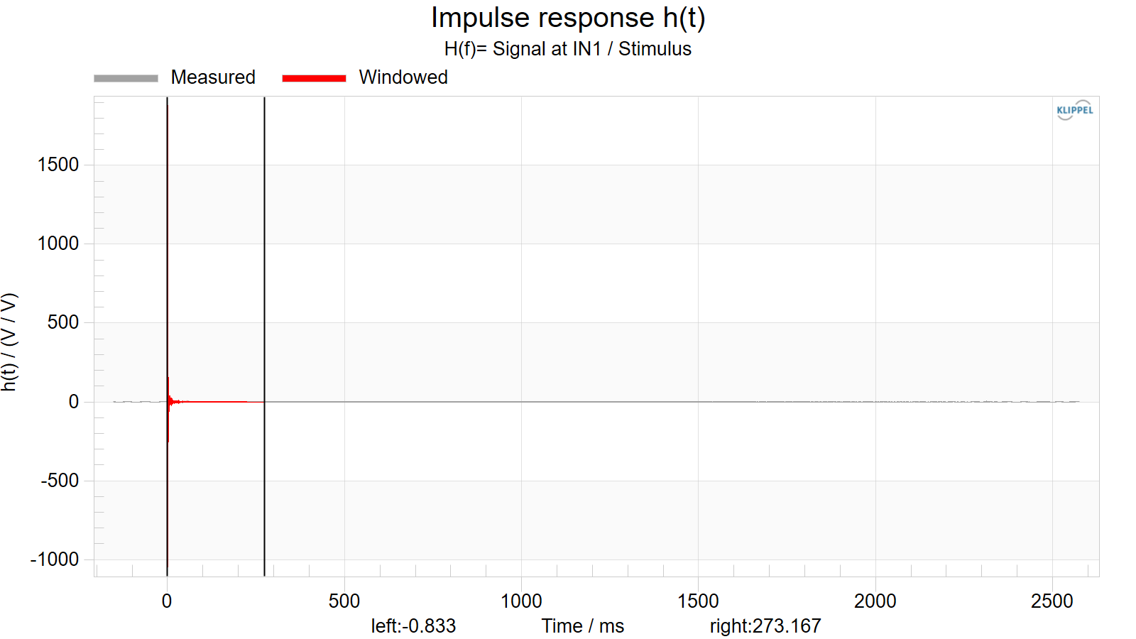
Shows the measured (gray) and the windowed (red) impulse response. Using the two black markers, a section of the impulse response can be selected for further analysis, e.g. to exclude room reflections. Use the mouse to drag the markers. Alternatively, press SHIFT and click the left mouse button at the desired position of the left marker. Press CTRL and click to set the right marker. Once the marker are moved the calculation of the transfer function is restarted. If a marker is moved into the region of nonlinear distortion it will be plotted dashed to warn the user. If you leave the marker in that position you might produce erroneous results. Hence, if a dashed marker appears change the marker position till you get a solid line marker.

Energy-Time Curve#

The energy-time curve (ETC) is the envelope of the impulse response given in dB. The curve is scaled in order to set the peak of the envelope to 0 dB. The measured ETC is shown as gray curve while the ETC inside the window is the red curve. For calculating the ETC no frequency domain window (like half-Hann, etc.) is applied. Sometimes the ETC shows the direct sound response more clearly than the impulse response. Furthermore the ETC is very useful to separate the linear and nonlinear part of the response. Normally the ETC decays on the right hand side of the linear impulse. After a certain point it rises again due to the nonlinear response. This points can clearly be seen in as minimum of the ETC. Left of the minimum is the linear part of the response and right of it starts the nonlinear one.

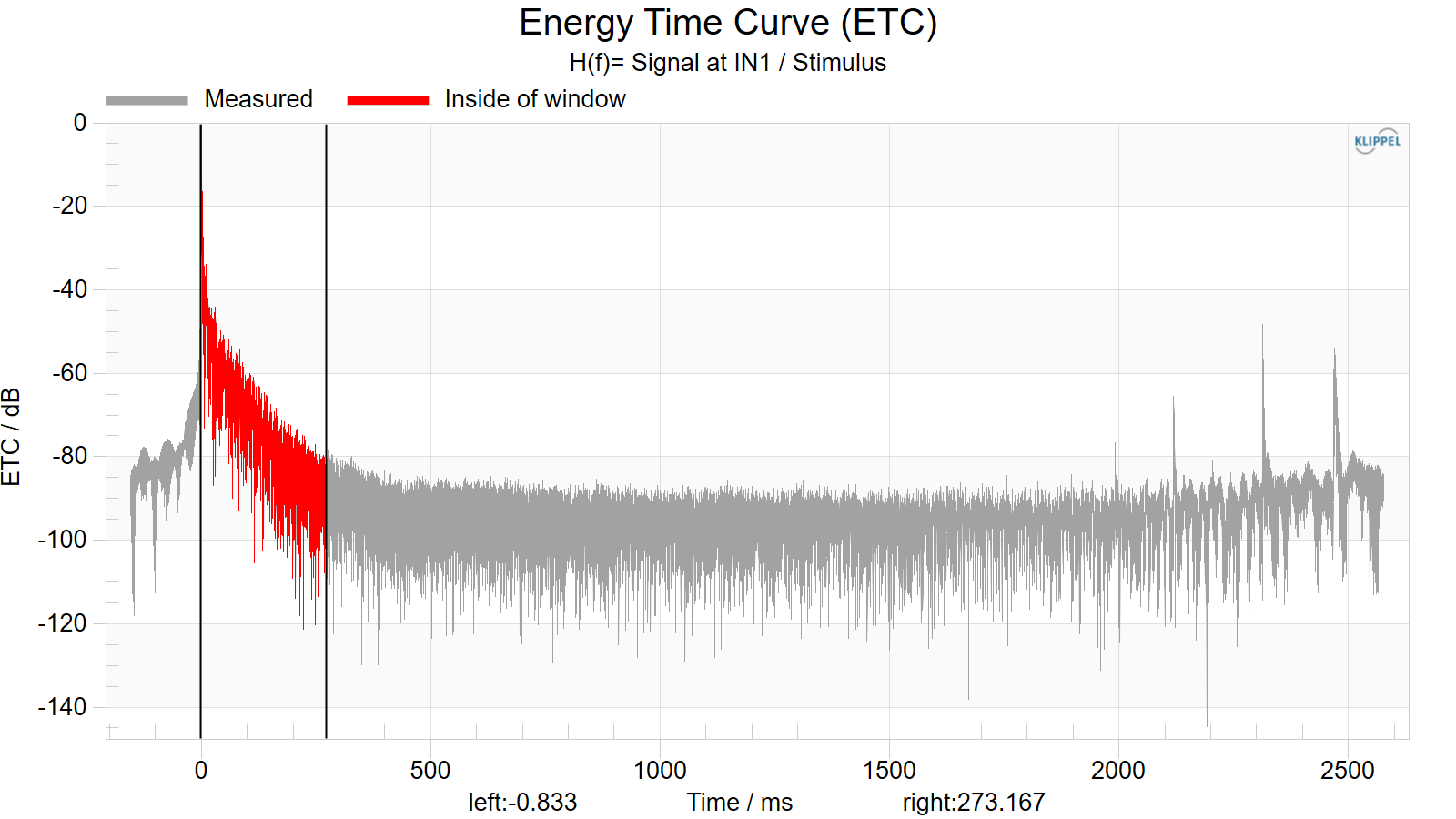
Using the two black markers a section of the ETC can be selected for further analysis. The two markers are totally synchronous to the markers in the result windows Impulse Response and Step Response. If the position of a marker is changes in the Impulse Response or Step Response window the position of the corresponding marker in the Energy-Time Curve window is changed as well and vice versa.

s(t) Step Response#

(with result overlay for unwindowed step response )

The step response is response of the system to a unit step excitation. It is calculated by integrating impulse response numerically. . The measured step response is shown as gray curve while the step response inside the window is the red curve.

Using the two black markers a section of the step response can be selected for further analysis. The two markers are totally synchronous to the markers in the result windows Impulse Response and ETC. If the position of a marker is changes in the Impulse Response or ETC window the position of the corresponding marker in the Step Response window is changed as well and vice versa.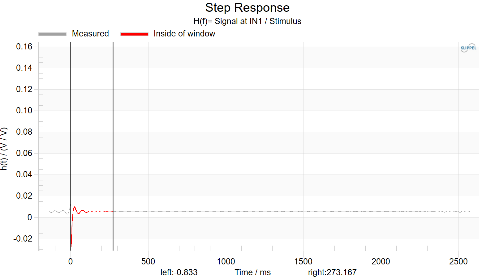

H(f) Magnitude#

(with result overlay)

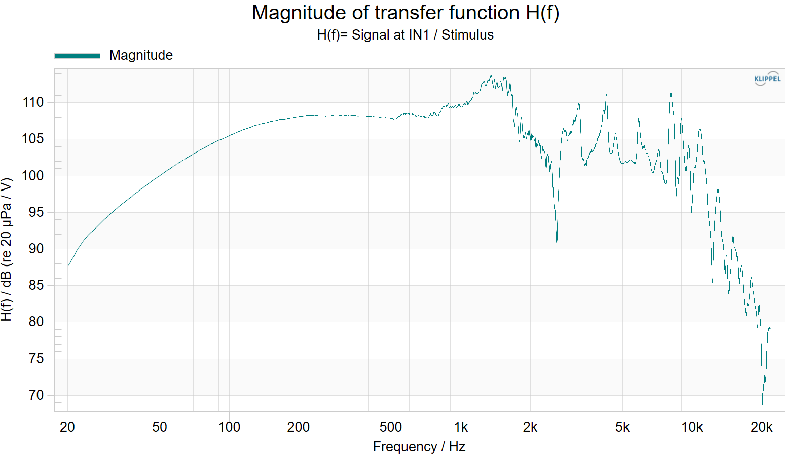
Shows the magnitude of the true transfer function, meaning that the two signals selected as numerator and denominator of the transfer function \(H(f)\) in property page Processing are divided by each other in the frequency domain.

Fundamental + Harmonic Distortion#

Note

(ID, Fund. Mean, ID limit & HOHD shown in TRF-Pro only)

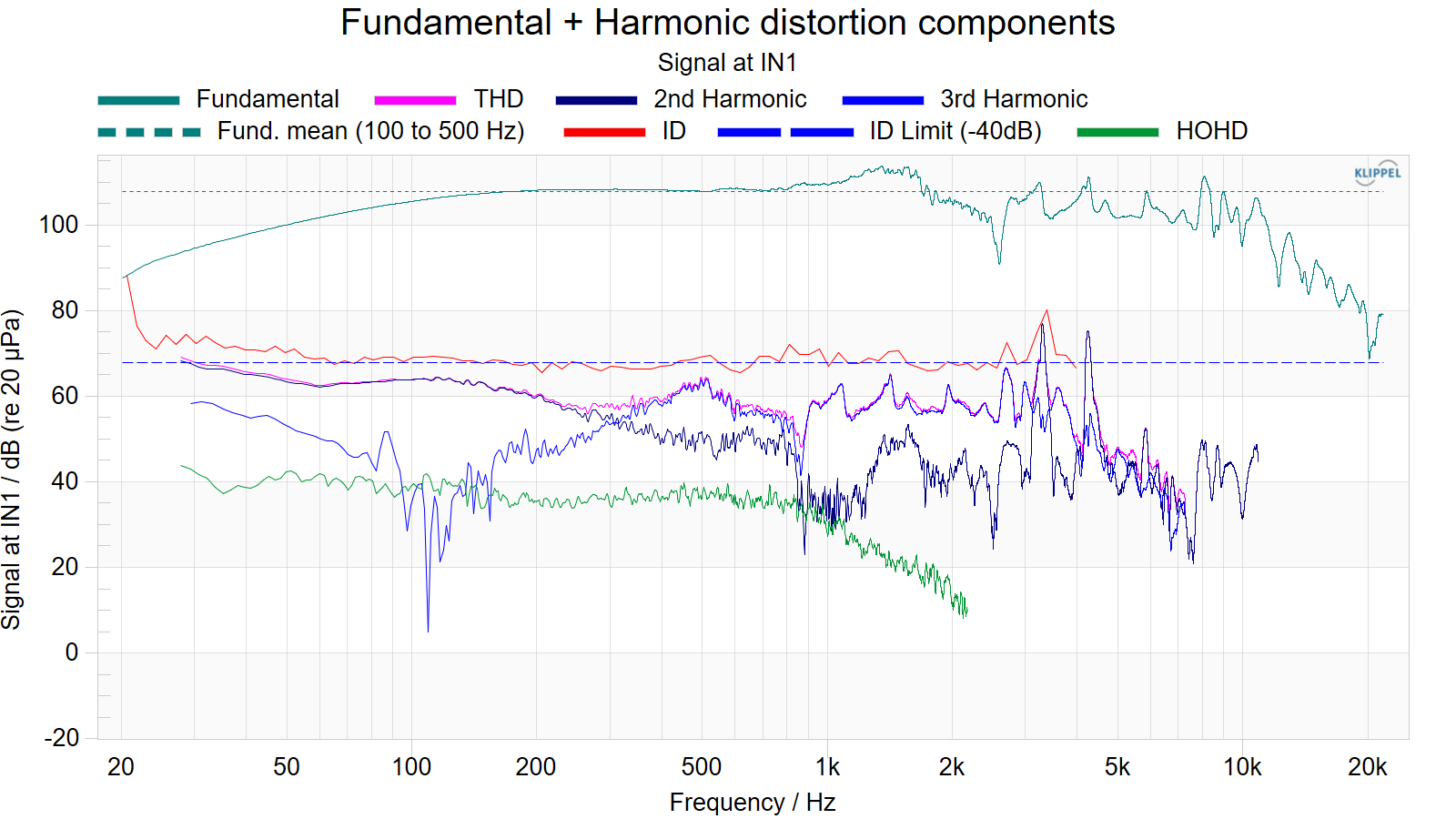
Shows the magnitudes of the fundamental, the total harmonic distortion (THD), the 2^nd and 3^rd order harmonic distortion components of the numerator signal of the transfer function. The THD is calculated using the following equation

\[THD = \frac{\sqrt{\sum_{n = 2}^{N_{\max}}{P(Nf)²}}}{P_{\text{ref}}(f)} \cdot 100\%\]

Note

The lowest frequency of the harmonic distortion is defined by the length of the automatic time windowing which is used to determine the harmonic distortion. This window depends on the sweep speed and length of the stimulus.

TRF-Pro only#

The Higher-order Harmonic Distortion (HOHD) are calculated according to the IEC60268-21 by:

\[P_{HOHD} = \frac{\sqrt{\sum_{n = N_{\min}}^{N_{\max}}{P(Nf)²}}}{P_{\text{ref}}(f)} \cdot 100\%\]

The maximum and minimum distortion order of the HOHD can be defined in the I-Dist Property Page

ID shows the Peak of the impulsive distortion (see section Distortion measures for further information).

Fundamental mean and ID limit are used to define a meaningful limit for the impulsive distortion ID. It is configured in in the Property Page I-Dist.

Fundamental mean is calculated using the following equation

\(L_{\text{mean}} = 10\log_{10}\left( \frac{\frac{1}{N}\sum_{i = 1}^{N}{{P_{0}}^{2}10^{L(f_{i})/10}}}{{P_{0}}^{2}} \right)\).

Display Configuration#

Results will be shown only if Stim is selected as transfer function denominator in property page Processing.

You can switch between absolute (rms) and relative (dB) display on property page Display. For relative display, the reference is the calibration value on property page Input..

The TRF module measures the harmonic distortion components up to the 24^th order. For clarity reasons only the 2^nd and 3^rd harmonics are displayed by default. If you want to view the higher order harmonics, right click and select Customization Dialog… ‣ Subsets from the popup menu. Select the harmonics you are interested in and click OK.

Harmonic distortion#

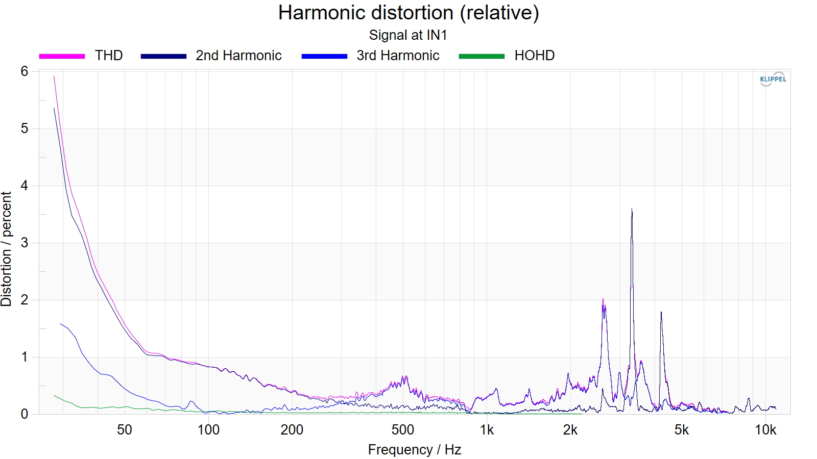
The result window shows the total harmonic distortion (THD)

\[d_{\text{THD}}(f) = \frac{ \sqrt{P(2f)^2 + P(3f)^2 + \ldots + P(24f)^2} } { \sqrt{ P(f)^2 + P(2f)^2 + P(3f)^2 + \ldots + P(24f)^2} } \cdot 100\%\]

as well as the 2^nd and 3^rd order harmonic distortion (d h2. and d h3.) of the numerator signal of the transfer function in percent

\[d_{\text{h}n}(f) = \frac{ P(nf) } { \sqrt{ P(f)^2 + P(2f)^2 + P(3f)^2 + \ldots + P(24f)^2} } \cdot 100\%\]

or dB (0 dB corresponds to 100 %) respectively.

Note

Results will be shown only if Stim is selected as transfer function denominator in property page Processing.

The TRF module measures the harmonics up to the 24^th order. For clarity reasons only the 2^nd and 3^rd harmonics are displayed by default. If you want to view the higher order harmonics, right click and select Customization Dialog… ‣ Subsets from the popup menu. Select the harmonics you are interested in and click OK.

TRF-Pro only#

Relative Higher-order Harmonic Distortion (HOHD) are calculated according to the IEC60268-21 by:

\[P_{HOHD} = \frac{\sqrt{\sum_{n = N_{\min}}^{N_{\max}}{P(Nf)²}}}{P_{\text{ref}}(f)} \cdot 100\%\]

The maximum and minimum distortion order of the HOHD can be defined in the I-Dist Property Page

Reference Curve#

Reference curve for the transfer function \(H(f)\) that can be imported in property page Processing

See also

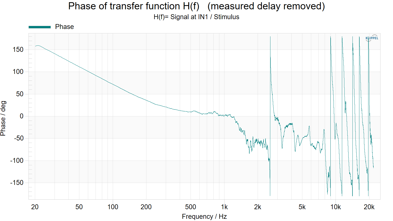
Using References / Comparing results

H(f) Phase#

(with result overlay)

Total phase of transfer function \(H(f)\). The phase can displayed wrapped and unwrapped as well as with and without time delay

See also

DISPLAY Page

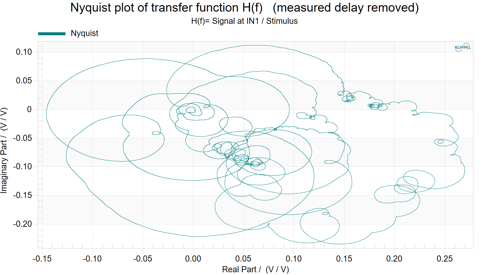
H(f) Nyquist#

(with result overlay)

Nyquist plot of transfer function \(H(f)\). It shows the imaginary part of \(H(f)\) vs. the real part of \(H(f)\). The Nyquist plot can displayed with and without time delay

See also

DISPLAY Page

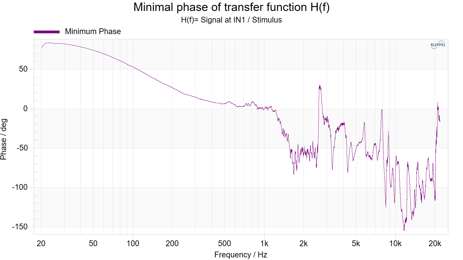
H(f) Minimum Phase#

(with result overlay)

Minimum phase of transfer function \(H(f)\). The minimum phase can displayed wrapped or unwrapped

See also

DISPLAY Page

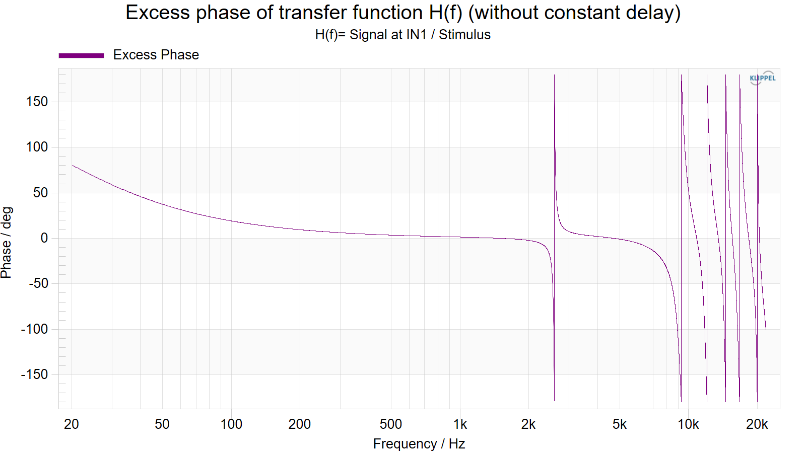
H(f) Excess Phase#

(with result overlay)

Excess phase of transfer function \(H(f)\). The excess phase is

φ = total phase of \(H(f)\) ‑ minimal phase ‑ effect of time delay.

The excess phase can displayed wrapped or unwrapped

See also

DISPLAY Page

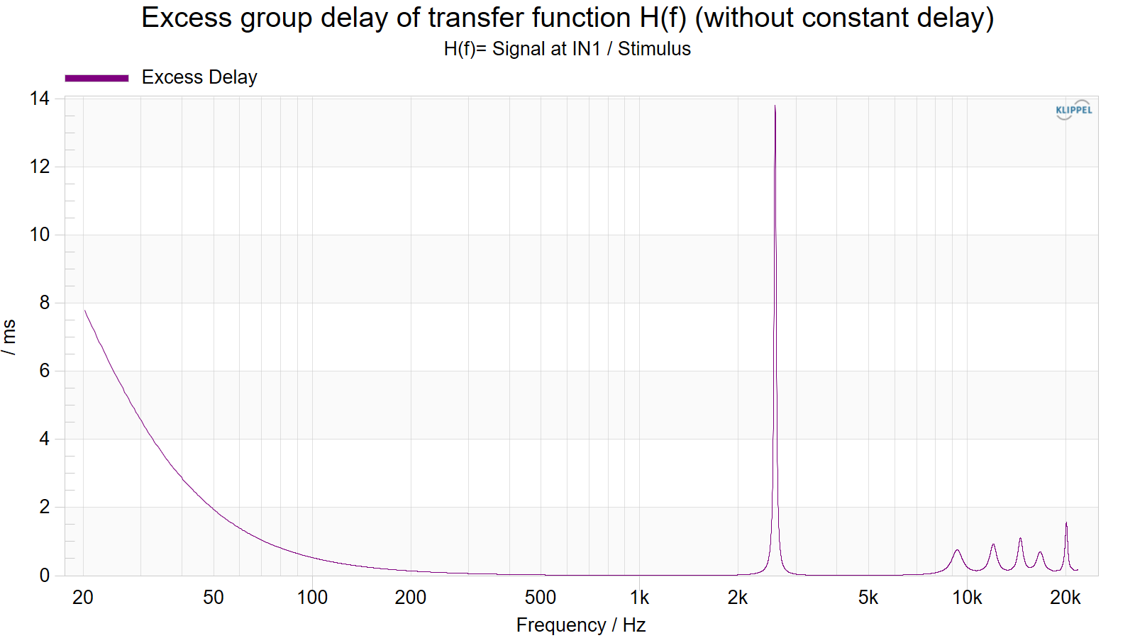
H(f) Excess Delay#

(with result overlay)

Excess delay of transfer function \(H(f)\). The excess delay is the negative derivative of the excess phase (result window H(f) Excess Phase).

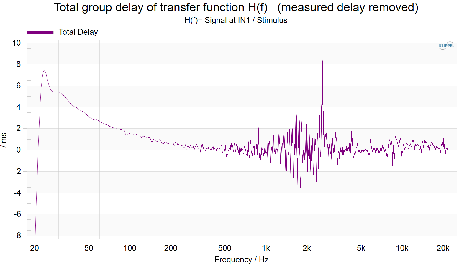
H(f) Group Delay#

(with result overlay)

Total delay of transfer function \(H(f)\). The total delay is the negative derivative of the (total) phase of the transfer function (result window H(f) Phase).

Cumulative Spectral Decay#

Cumulative spectral decay (CSD) for transfer function \(H(f)\). The cumulative spectral decay plot illustrates the decay of the individual frequency components after a sinusoidal excitation is suddenly switched off.

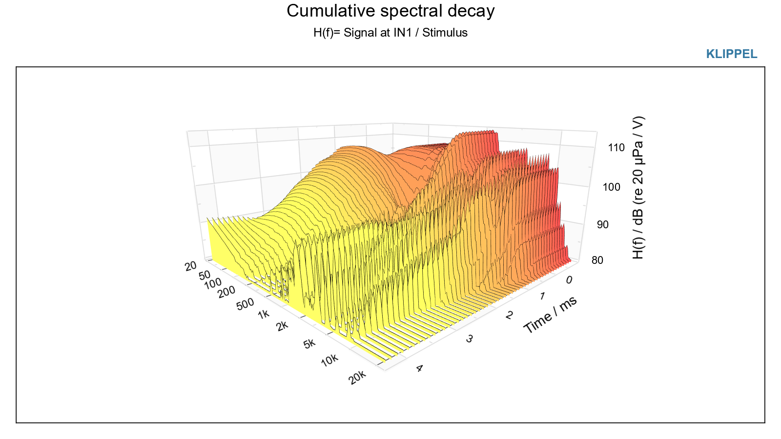
The ”time slices” for which the decay is plotted vs. frequency are specified in property page 3D. Slices determines the number of “time slices” while Shift is the distance between the individual slices.

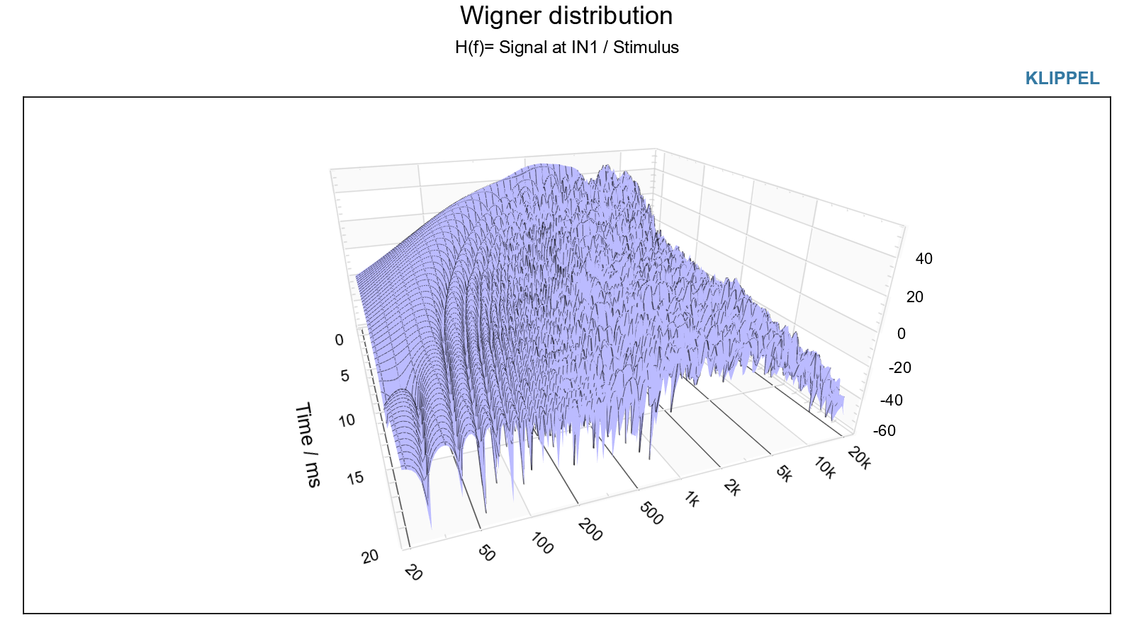
Wigner Distribution#

Wigner distribution the transfer function \(H(f)\). The Wigner distribution shows the “energy” present in the signal vs. frequency and time.

Use property page 3D to adjust the plot. Slices determines the number of “time slices” while Shift is the distance between the individual slices.

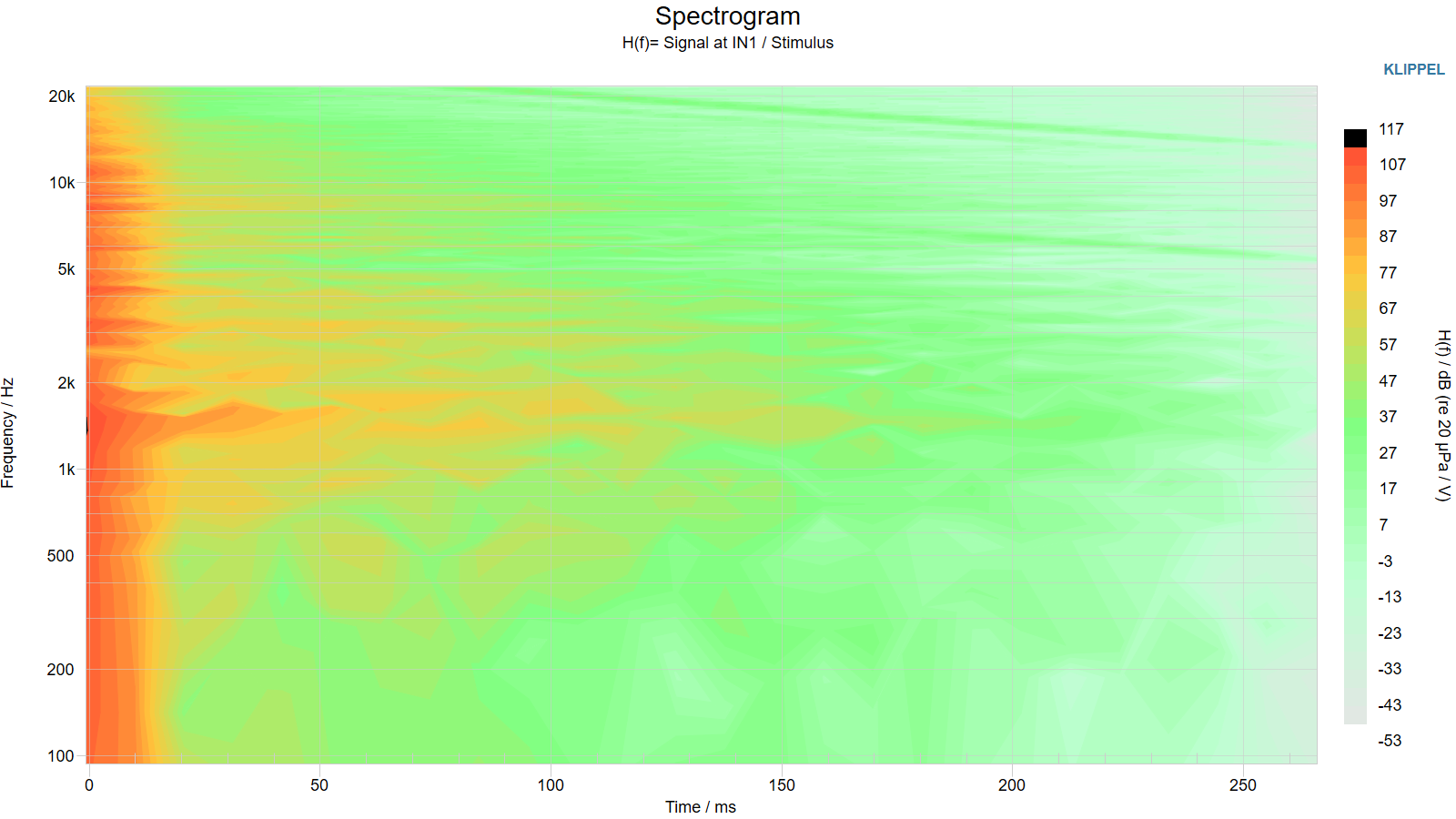
Spectrogram#

The plot shows the results of a sequence of short time FFTs. A short symmetric data window is used to separate subsequent overlapping sections of the direct sounds impulse response. After that each section is subjected to a FFT. These FFT results are displayed together in a 3D plot. Use property page Processing to control the plot. Slices determines the number of sections to be analyzed and FFT is the corresponding size of the short time FFT. The FFT size depends on the parameter Slices and the distance between the markers in result window Impulse Response. To use other methods for the time frequency analysis e.g. Wavelet transform or a filter bank the Time Frequency Analysis module (TFA) can be used.

Stimulus Spectrum#

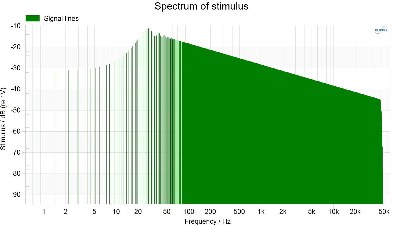
Shows the spectral lines of the stimulus. Use that result window to check the effect of an imported stimulus shaping curve

See also

STIMULUS Page

Y1(f) Input Spectrum#

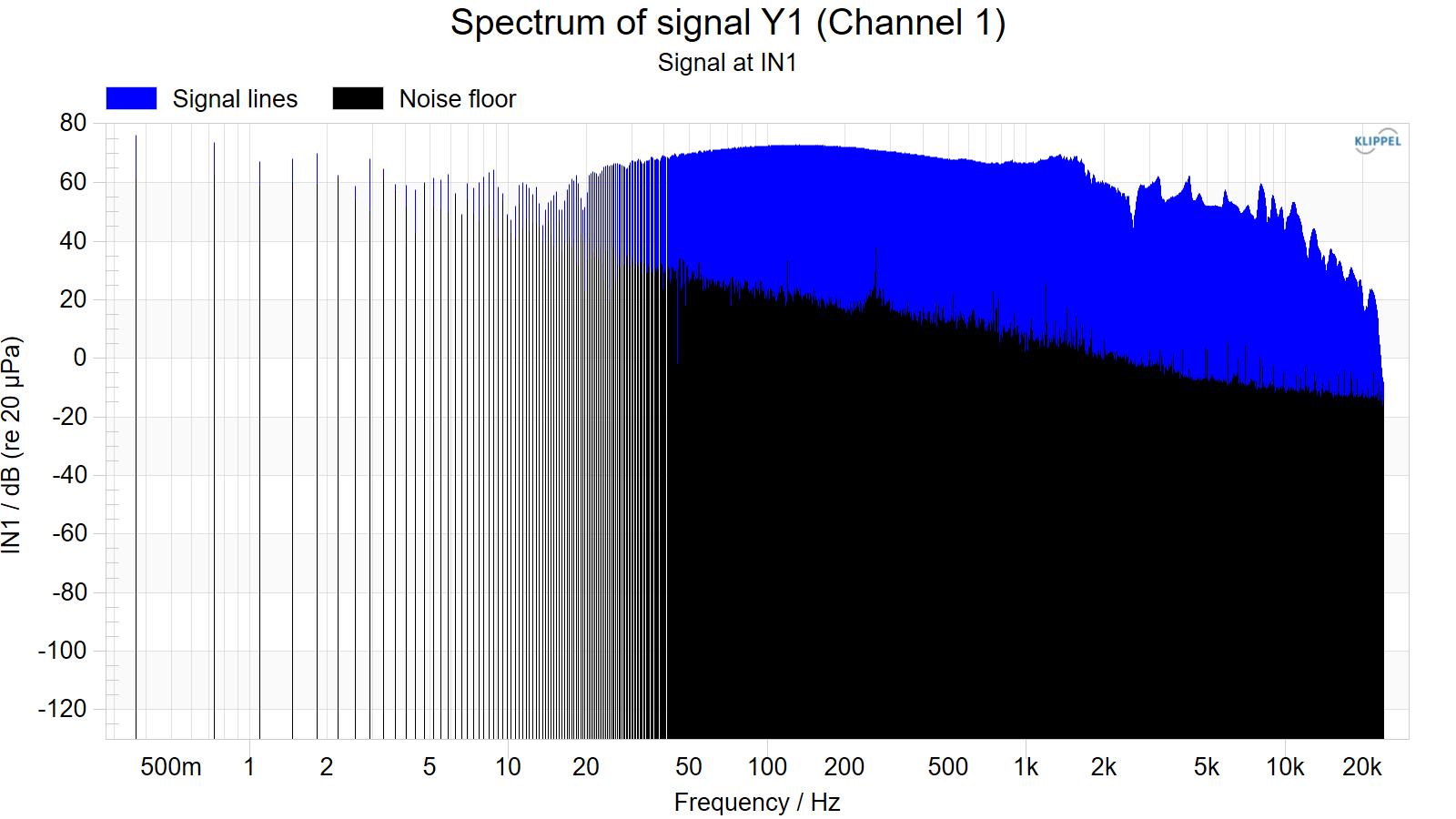
Shows the spectral lines (blue lines) of the signal Y1 acquired on channel 1. If the option Noise floor monitoring was selected in property page Stimulus. The spectral lines of the noise floor are plotted as black lines. There are several display modes that are selected in property page Display.

See also

DISPLAY Page

Y2(f) Input Spectrum#

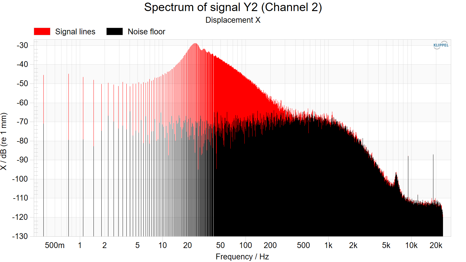
Shows the spectral lines (red lines) of the signal Y2 acquired on channel 2. If the option Noise floor monitoring was selected in property page Stimulus the spectral lines of the noise floor are plotted as black lines.

See also

DISPLAY Page

Calibration Curves#

Shows the calibration curves for the signals Y1 and Y2 measured on channel 1 and channel 2 respectively. A calibration curve can be imported in property page Input for each physical signal (IN1, IN2, \(U_s\), \(I_s\), X). The plot shows the calibration curves for the two currently selected signals Y1 and Y2.

Stimulus Waveform#

Waveform of stimulus signal.

y1(t) Input Waveform#

Waveform of signal Y1 measured on channel 1.

y2(t) Input Waveform#

Waveform of signal Y2 measured on channel 2.

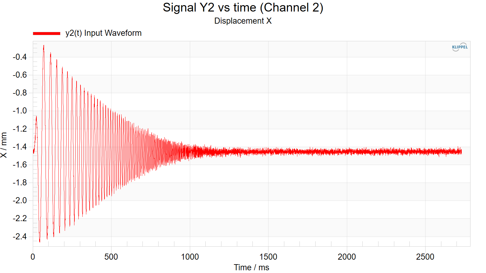
Table Results + Settings#

Collection of important result and setup parameters like time delay, measured amplifier gain and marker positions.

Instantaneous Distortion#

(TRF Pro only)

The window shows the instantaneous distortion versus frequency (red curve). Contrary to the traditional distortion measures like THD the instantaneous distortion reveal the full distortion fine structure. This is for instance useful to detect rub and buzz phenomena.

Note

Results will be shown only if Reference Curve is deactivated and Stimulus is selected as transfer function denominator in property page Processing.

The following distortion measures can be plotted

Mean impulsive distortion (MID)
Instantaneous impulsive distortion (IID)
Instantaneous crest of impulsive distortion (CID)
Impulsive distortion (ID)
Crest of impulsive distortion (CID)

The particular distortion measure to be plotted and is selected in property page I‑Dist (combobox Measure). The distortion are displayed in percent or in dB (100 % corresponds to 0 dB) depending on the selection property page I‑Dist.

In case the instantaneous distortion are measured with a reference driver (“golden unit”) the measurement noise floor is calculated and plotted as black curve. To show the deviation of the distortion from the noise floor select Show distortion to noise ratio in property page I‑Dist. In this case the ratio of distortion and noise level will be plotted as blue curve.

Note

Three learning cycles are needed to calculate the noise floor.

See also

I-DIST Page
Instantaneous Distortion
Distortion measures

Instantaneous Distortion 3D#

(TRF Pro only)

For Rub & Buzz measurement the TRF has special visualization which combines the displacement with the instantaneous crest of the higher order distortion. For more information about Rub & Buzz measurements with the TRF module see Application Note 22 and 23.

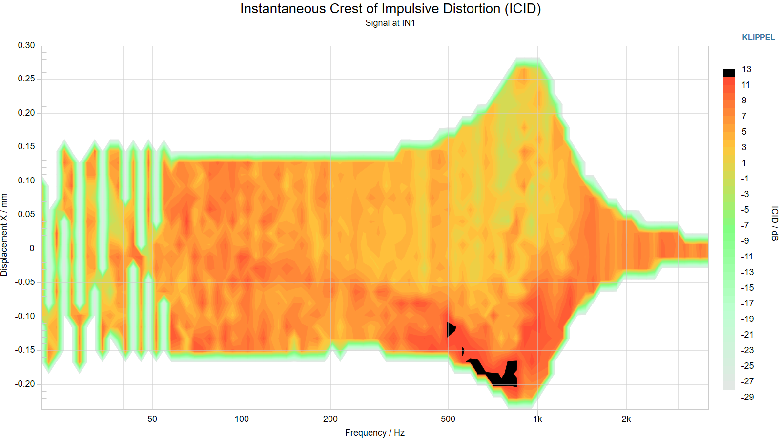
To ensure a valid mapping the displacement signal of the Laser must be synchronized with sound pressure input of the microphone. The currently recommended Keyence laser sensors have built-in digital signal processing and therefore there is a significant time delay compared to the microphone signal. Since in the 3D graph both signals are overlaid you have to ensure correct time delay compensation in property page Processing. Otherwise the black spots may occur at wrong displacement values.

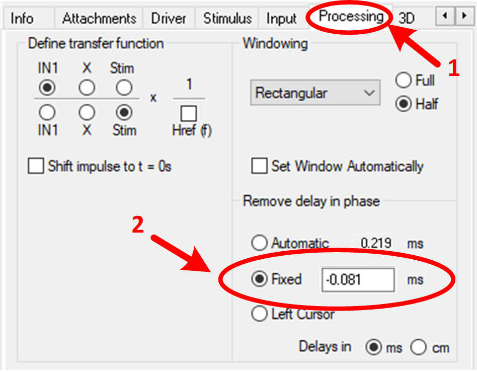
\(\Delta t_{\text{mic}}-\Delta t_{\text{remove}} = \Delta t_{\text{laser}}\)

with

\(\Delta t_{\text{mic}}\): measured Mic delay
\(\Delta t_{\text{remove}}\): calculated remove delay
\(\Delta t_{\text{laser}}\): laser delay

the used laser in this example is LK-G32 which has a time delay of 0.3 ms. The measured Mic delay is 0.219 ms. So the removed delay can be calculated as: 0.219-0.3 = -0.081 ms

The known time delay values for different Keyence lasers are listed as follows:

LK-H052 / 022 / 082 (with Klippel setting) = 580 +/- 10 µs
LK-G32 / 82 (with Fmax 10kHz Klippel setting) = 120 µs
LK-G32 / 82 (with Fmax 25kHz Klippel setting) = 300 µs

The window shows the instantaneous distortion as contour (color) in the 3rd dimension. The x-axis shows the excitation frequency while the y-axis maps the distortion to the channel 1 (or channel 2) measurement signal (for the instance instantaneous displacement of the voice coil). The y‑axis signal is selected in property page I‑Dist. The color corresponds to the distortion level. The coloring can be controlled with the threshold Thresh in property page I‑Dist. Areas in which the distortion exceeds the threshold are plotted black.

The y-axis mapping is very useful to find the causes of rub & buzz. Often the voice coil excursion at which the rub & buzz occurs gives valuable hints. If for instance the voice coil hits slightly against the back plate, distortions are produced at negative (inside) peak displacements.

Note

Results will be shown only if Reference Curve is deactivated and Stimulus is selected as transfer function denominator in property page Processing.

The following distortion measures can be plotted:

Mean impulsive distortion (MID)
Instantaneous impulsive distortion (IID)
Instantaneous crest of impulsive distortion (CID)
Impulsive distortion (ID)
Crest of impulsive distortion (CID)

The particular distortion measure to be plotted and is selected in property page I‑Dist (combobox Measure). The distortion are displayed in percent or in dB (100 % corresponds to 0 dB) depending on the selection property page I‑Dist.

In case the instantaneous distortions are measured with a reference driver (“golden unit”) the measurement noise floor is calculated. To show the deviation of the distortion from the noise floor select Show distortion to noise ratio in property page I‑Dist.

Modeled Response#

(TRF Pro only)

The result window shows the measured non-processed waveform (blue curve) and the corresponding modeled waveform (gray curve). The difference between both time signals is the residual signal e(t) (red curve). The various instantaneous distortion measures are calculated from the residual signal e(t) and the measured waveforms. The waveforms are shown in two different windows over the instantaneous frequency to check at which frequency the rub and buzz effects happen and over the time to extract and auralize the rub and buzz effects.

Note

Results will be shown only if Reference Curve is deactivated and Stim is selected as transfer function denominator in property page Processing.

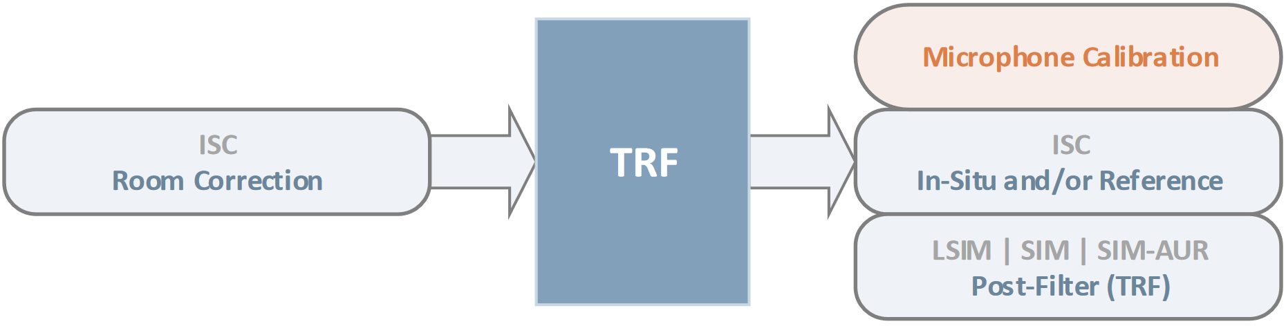
Supported Modules for Im/Export#

Measurement of instantaneous distortion#

The traditional distortion measurement transforms the time signal into the frequency domain to separate fundamental, harmonic and intermodulation components. This technique considers only the mean power in the analyzed interval and neglects the phase information. The TRF Pro supports a new technique for the measurement of the signal distortion in time domain that exploits both amplitude and phase information. It reveals the fine structure of the distortion and its dependency on frequency, displacement or other state variables. Besides the rms-value of the distortion the peak value and the crest factor are important characteristics for detection of rub and buzz phenomena.

Isolating rub & buzz distortion#

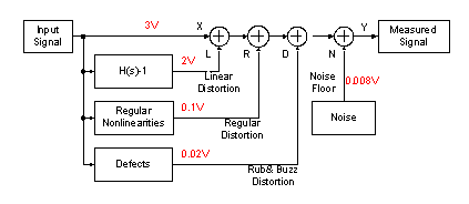
Several distortion components contribute to the measured output signal of a speaker. As illustrated below, the components contribute at different levels. Linear distortion L caused by the amplitude and phase response is much higher than regular distortion R caused by motor and suspension nonlinearities. Distortion D caused by loudspeaker defects are even lower. After all a certain level of noise N is always added to the measured signal. Noise has no correlation with the input signal but can be characterized as a contribution of energy (noise floor). Rub & buzz effects D are usually masked by linear distortion L and regular distortion R.

Time domain analysis#

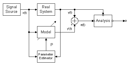
The parameters of a dedicated loudspeaker model are identified by analyzing the signals excitation X(t) and y(t). The model is used to reproduce the linear distortion L and the regular distortion R of the driver. The excitation signal X(t) generates the loudspeaker output signal y(t). The same excitation is applied to the identified model. The model output signal y’(t) comprises the linear distortion L as well as the regular distortion R which are part of the design and do not contribute to rub and buzz effects D. The difference e(t) of both signals holds all information about the distortion D.

Using a “golden unit”#

If a reference driver (“golden unit”) is available it can be used to identify the parameter of the models. In this the model reproduced the linear and regular distortion (L+R) of the reference driver and the measurement will show any deviation from the behavior of the reference.

Distortion measures#

Several distortion measures are supported. They are all calculated by post-processing the residual signal e(t) and the measured output signal y(t) of the driver.

MID (Mean impulsive distortion), according to IEC 60268-21#

Absolute: \[\text{MID}(f(t)) = 20 \log \left(e_{\text{RMS}} / p_0 \right)\]
Relative: \[d_{\text{MID}}(f(t)) = \frac{e_{\text{RMS}}}{y_{\text{RMS}}}\]

IID (Instantaneous impulsive distortion)#

Absolute: \[\text{IID}(f(t)) = 20 \log \left( \left| e\left( t \right) \right| / p_0 \right)\]
Relative: \[d_{\text{IID}}(f(t)) = \frac{\left| e\left( t \right) \right|}{y_{\text{RMS}}}\]

ID (Impulsive distortion), according to IEC 60268-21#

Absolute: \[\text{ID}(f(t)) = 20 \log \left( e_{\text{peak}} / p_0 \right)\]
Relative: \[d_{\text{ID}}(f(t)) = \frac{e_{\text{peak}}}{y_{\text{RMS}}}\]

Crest Factor Definitions, according to IEC 60268-21#

CHD (Crest of impulsive distortion): \[\text{CID}(f(t)) = \frac{e_{\text{peak}}}{e_{\text{RMS}}} = \text{ID}(f(t)) - \text{MID}(f(t))\]
ICID (Instantaneous crest of impulsive distortion): \[d_{\text{ICID}}(f(t)) = \frac{\left| e\left( t \right) \right|}{e_{\text{RMS}}}\]

Definition of yRMS, eRMS, epeak#

\[y_{\text{RMS}} = \sqrt{\frac{1}{t_{k+1}-t_k} \int_{t_k}^{t_{k-1}}y^2(t)dt }\]

\[e_{\text{RMS}} = \sqrt{\frac{1}{t_{k+1}-t_k} \int_{t_k}^{t_{k-1}}e^2(t)dt }\]

are the RMS of y(t) and e(t) values of a k-th time shred with \(k= 0\ldots N-2\).

\(N\) denotes the number of shreds for the complete time signal and

\[e_{\text{peak}} = \max_{t_k\leq t\lt t_{k-1}}\left[ \left| e(t) \right| \right]\]

is the absolute peak value of the k-th time shred. The above equations give the distortion measures versus measurement time.

Since the TRF module uses sine sweep excitation there is a unique mapping between time and instantaneous excitation frequency. It is therefore straight forward to plot the distortion measures versus frequency.

Curve import and export#

The required format for curve export and import is quite simple. The same format is generally used within the Klippel R&D System for importing or exporting curves from or to the clipboard. Each curve is represented by two columns of ASCII numbers. The columns are separated by blanks, rows are separated by line breaks. The first column contains the x-values (e.g. frequency), the second column contains the y-values (e.g. dB); see example below. Each row represents a base point of the curve. The fractional part of the x- and y-values must be separated by a dot, comma is not allowed. Any external text editor can be used to type in the two columns. If you select them with the mouse and press [Ctrl + C] they are copied to the clipboard. Alternatively use the clipboard editor provided by dB-Lab. It is activated by choosing View ‣ Clipboard in the menu. Between the base points the curve is interpolated linearly. Outside the base point range the value of the first and the last base point is used respectively.

Example#

The curve consists of following the five points:

(20 Hz, 0 dB), (1 kHz, -3.8 dB), (2 kHz, -1.2 dB), (5 kHz, 2.5 dB), (10 kHz, 0 dB)

The corresponding clipboard format is:

   0.0
 -3.8
 -1.2
 2.5
0.0

Malfunction and Troubleshooting#

Overview#

This chapter will provide information that can help you solve common problems that occur with the Distortion Analyzer and the TRF module. The software generates a variety of warnings automatically if the signals are badly conditioned or a malfunction is detected. Some warnings may be neglected but it is always recommended to find out the cause of the problem.

If you cannot find a description here that matches your problem, try these options:

Check the file readme.txt that you received with your Distortion Analyzer products. This document contains the most up-to-date information about products and installation procedures.

Contact us via KLIPPEL support.

See also

dB-Lab Malfunction and Troubleshooting

Error and Warning Messages#

Primary data is already available#

Measurement results will be deleted if the corresponding setup parameter are changed. This way results and setup parameter are kept consistent. If you want to perform a new measurement while preserving the old results, please create a new operation. The setup parameters of the old measurement can be conveniently copied to new operation with the Copy and Paste buttons that you find on property page IM/EXPORT Page. Furthermore you can save the Setup of the operation as Template for new operations.

WARNING: Stimulus is applied to OUT 1(2)#

This warning will be generated if at OUT 1 or at OUT 2 is selected in the group Voltage in property page Stimulus. In this case the specified stimulus voltage is the voltage at the output connector OUT 1 or OUT 2 (and hence at the amplifier input if an amplifier is connected).

Warning

The level of the amplifier output signal can be considerably higher than the specified level and can possibly destroy your speaker!

No proper amplifier output#

The amplifier is tested before the main measurement. During this test the gain is measured at 750 Hz. The error message is generated if the amplifier is switched off or if the test signal is not transmitted properly.

General amplifier output error#

Error

No proper amplifier output!
SNR lower than 35dB
Check amplifier power, KA3 Signal routing, and cables

No proper amplifier output!
SNR lower than 35dB

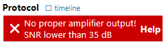
Remedy

Check the amplifier.
Check the SNR of the test signal at 750 Hz in result window Y1(f) Input Spectrum.
- The SNR should be at least 35 dB for the 750 Hz line. Increase the amplifier gain.
Check the connection and the cables in the hardware setup.
- Is the amplifier input connected to the output (OUT 1 or OUT 2) that is selected in property page STIMULUS Page?
- Is speaker cable connected to the speaker connector that is selected in property page INPUT Page?
KA3: Is the dedicated Output selected at the KA3 Signal Configuration?

KA3 Power Cycling Error#

Error

No proper amplifier output!
SNR lower than 35dB
Amplifier card output failure. Power cycle the KA3 device. And run the measurement again.

Remedy

If the KA3 Amp Card is used, It could hang requiring a power cycling of the KA3.

Desired excitation level cannot be realized#

This error message is generated if the gain is too small to realize the desired excitation level.

Remedy

Increase the amplifier gain.
- Use an amplifier if you did not use one so far.
- Switch to at Speaker terminals in property page STIMULUS Page.
- Decrease excitation level to the value shown in the message box.

No proper calibrator signal#

This message is generated if the calibrator (pistonphone) signal does not exceed any other signal component by at least 25 dB.

Remedy

Check your calibrator and the hardware connections.
If you are calibrating the first channel, check the result windows Y1(t) and Y1(f) Spectrum for any humming component or other irregularity.
Check Y2(t) and Y2(f) Spectrum if you are calibrating the second channel.

Channel x signal is limiting#

The signal acquired on channel 1 or 2 is limiting.

Remedy

Reduce excitation level or increase the headroom expansion for the channel in property page INPUT Page.

Negative Sensitivity is not supported#

The TRF module does not support sensors with a negative sensitivity. Please check the selected sensors in the signal configuration (see KA3, DA2) Define a positive sensitivity in the sensor file and use the microphone reference curve invert the signal by applying a filter with 180° phase shift.

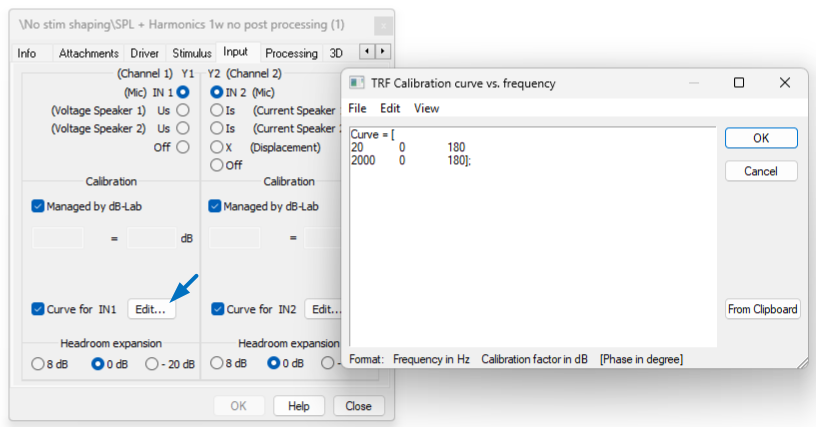
WARNING: Stored model for inst. dist. not compatible#

The model for the instantaneous distortion measurement was learned using different measurement setting than the settings of the actual measurement. You have changed one or more of the following setup parameters:

Stimulus
- Fmin
- Fmax
- Resolution
- excitation level
Processing
- numerator of transfer function
- denominator signal of transfer function
I-Dist
- Mode

Remedy

The model is not valid anymore and should be discarded.
Alternatively you can keep the model and set the changed setup parameters to its original values.

High Sensitivity current sensor selected#

Warning: High Sensitivity current sensor selected: Voltage at the DUT (speaker) could be lower than specified, due to the used shunt resistor.

The current sensing shunt resistor used to get the best possible SNR in the current signal is placed in series to the DUT. Depending on the DUT’s impedance the shunt resistor causes a frequency depending voltage reduction at the DUT.

Remedy

If voltage reduction should be avoided
- open KA3 Signal Configuration
- Select the Low Sensitivity hall effect current sensor

Note

This warning is KA3 related. At High Sensitivity modified DA2s it will not be displayed.

TRF – Transfer Function Measurement

On this page

TRF – Transfer Function Measurement#

TRF Tutorial#

Overview#

What is the goal of this tutorial?#

Viewing TRF Results (Part 1)#

Stimulus Waveform#

First channel: Sound pressure response#

Impulse Response#

Windowing#

Fundamental + Harmonic Distortion#

H(f) Magnitude#

Second Channel: Displacement#

Performing a new TRF (Part 2)#

SPL Measurement#

Hardware Setup#

Create Operation#

Measurement Setup#

Start Measurement#

Viewing results#

Using Template#

Impedance Measurement#

Hardware Setup#

Create Operation#

Measurement Setup#

Result windows#

Property page Display#

Customizing TRF (Part 3)#

SPL Calibration#

Using a Pistonphone#

Manual Definition of Sensitivity#

How to load a Microphone Correction Curve?#

Export Transfer Function Data#

Result Overlay#

Modes of Operation#

Using References / Comparing results#

How to View Higher Order Harmonics?#

How to Speed up Marker Placement?#

How to measure instantaneous distortion?#

TRF Reference#

Overview#

Property pages#

STIMULUS Page#

Frequency#

Shaping#

Voltage#

Noise floor + dc monitoring#

Preloops#

Averaging#

Single Sweep#

Asynchronous measurement#

Export Stimulus#

Device Measurement Capabilities#

INPUT Page#

Y1 (Channel 1)#

Y2 (Channel 2)#

Calibration#

Headroom expansion#

PROCESSING Page#

Define transfer function#

Shift impulse to t = 0s#

Reference filter#

Windowing#

Remove Time Delay in phase#

3D Page#

Window#

Cumulative decay#

Wigner distribution#

Spectrogram#

DISPLAY Page#

Spectra#

Harmonic distortion#

Transfer function + 3D plots#

Unwrap phases#

IM/EXPORT Page#

Setup#

Transfer function#

I-DIST Page#

Mode#