SIM-AUR – Nonlinear Simulation and Auralization

SIM-AUR Tutorial

Overview

The Simulation Auralization (SIM‑AUR) module performs numerical simulations of electro-dynamical transducer, mounted in common enclosure systems. In addition to the objective measures, based on the simulation data the transducer and system can be auralized. The simulation technique features a dynamic thermal model, allowing the exploitation of the driver performance in simulated long-term applications. In contrary to the Simulation 2.0 (SIM) module, the input stimulus of the SIM‑AUR is based on waveform data, and can be of any kind of signal (e.g. test signals, music, …) and arbitrary length. The module uses an extended lumped-parameter model to describe the transfer behavior in the full working range. Electrical, mechanical, acoustical and thermal state variables are calculated and available for extended analysis.

To speed up prediction of the long‑term behavior, an optional time‑lapse technique is provided. This allows to easily find critical sections in the test signals, which can be simulated with higher precision to evaluate distortion and other measures.

In addition, nonlinear effects can be separated without affecting the simulated transducer system. This separation of the distortion in the acoustical output signal from the linear component is the basis for a new auralization technique. With this technique, double blind A/B comparisons may be performed, allowing the determination of the threshold of audibility systematically.

What is the Goal of This Tutorial?

This tutorial makes you familiar with the SIM~AUR module. It is divided into two parts:

1. In the first part, Viewing SIM-AUR Results, we will show how to view SIM-AUR results which are already stored in the web example database.

2. In the second part of the tutorial, Performing a SIM-AUR operation, a step-by-step recipe is provided to predict the long term performance of the speaker, find sections of interests and auralize these.

For detailed information about the background of the simulation, see section SIM‑AUR Reference. There, the nonlinear transducer model, the Time-lapse Technique as well as a detailed description of the result windows and the configuration of the property pages is provided.

Viewing SIM-AUR Results

SIM-AUR Simulation

Example data used in this manual is stored in the Web Example database. If not downloaded already, get it from the latest R&D release <https://www.klippel.de/go/current-rnd-release> and open the web-based database.

See also

View Results for general information on how to download this database, open and view results in dB-Lab.

1. Open the folder Simulation, Auralization (LSIM, SIM, SIM-AUR, DIF-AUR, ALS)\Simulation Auralization (SIM-AUR)\Simulation.

2. Open the object Microspeaker and double click the operation 1 SIM‑AUR Simulation.

3. After double clicking the operation, the default result windows will be opened. First, we will have a look at the parameters of the used driver model. We assume that an electro-dynamic loudspeaker can be modeled by an equivalent circuit.

   In the window Table Model Parameters you will find a brief overview of all model parameters used for the simulation. The section “Linear Transducer Parameters” show the linear (small-signal) parameters of the driver. With these parameters, the linear part of the driver is fully specified.

   

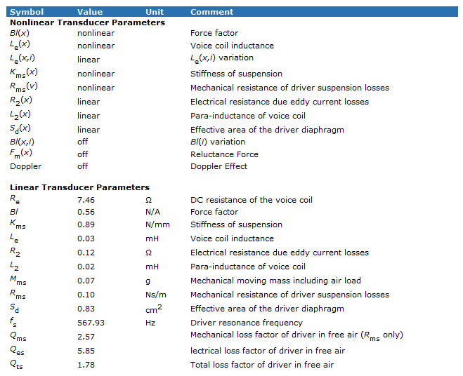
   The most important parameters are:

   R_e

   DC resistance of voice coil

   L_e

   Frequency independent part of the voice coil inductance

   Bl

   Force factor

   K_ms

   Mechanical stiffness

   f_s

   Driver resonance frequency

   Q_ms

   Mechanical loss factor

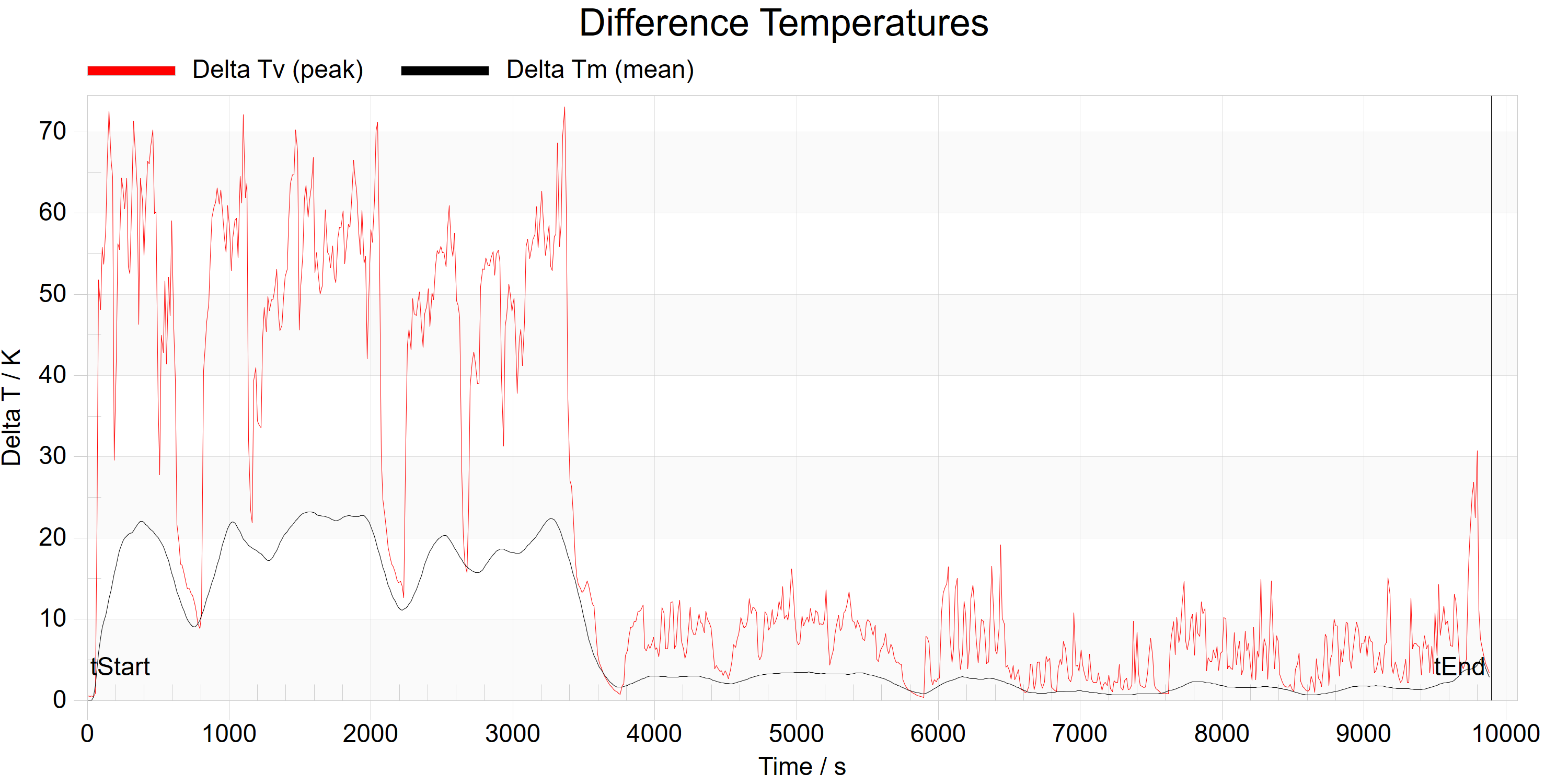
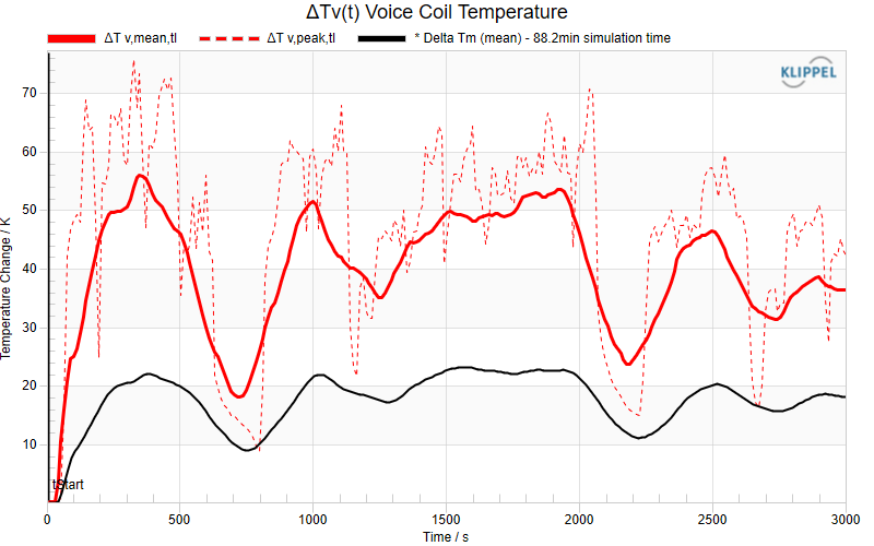
4. Inspecting the window Temperature, you will see the long-term temperature behavior. The red curve annotates the voice-coil temperature ΔT_v over time, whereas the black curve shows the increase of magnet temperature ΔT_m over time.

   

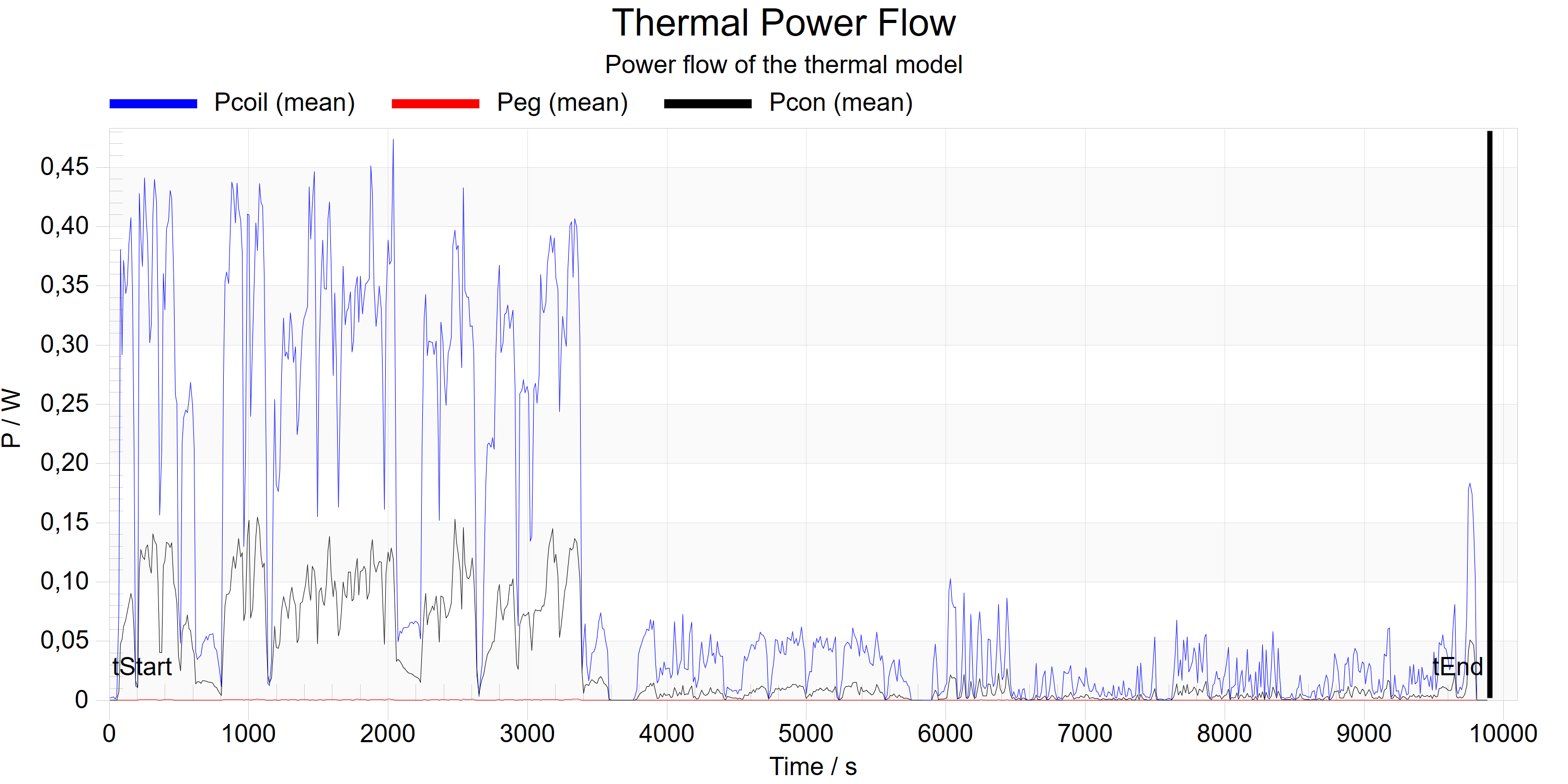
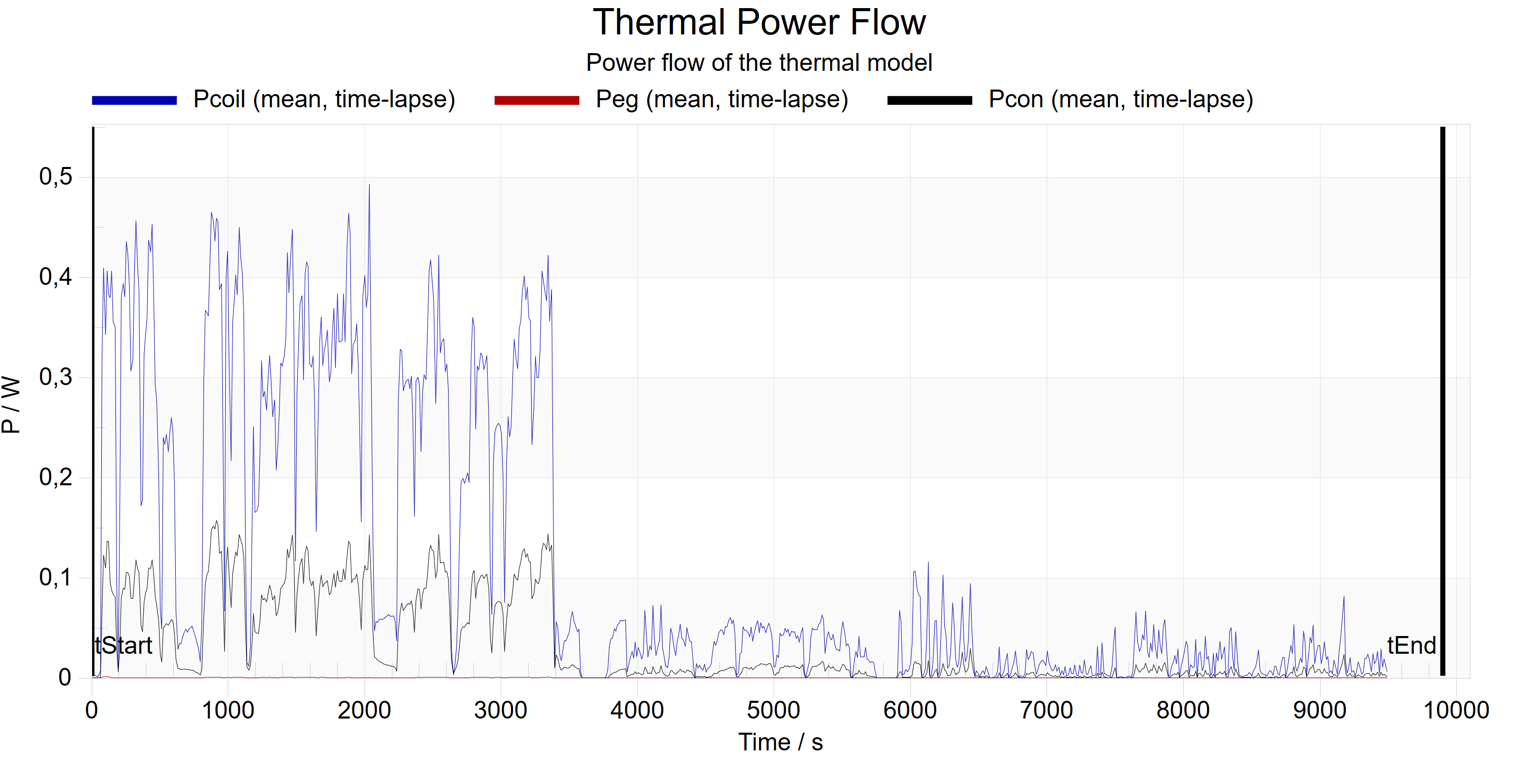
5. The window Thermal Power Flow shows the flow of the dissipated power of the simulated transducer. Using this information, a detailed insight in the thermal transducer behavior is possible. \(P_{coil}\) represents the power dissipated over the voice-coil, \(P_{eg}\) shows the power dissipated due eddy currents, and \(P_{con}\) represents the power which is transmitted to the surrounding air by convection cooling processes.

   

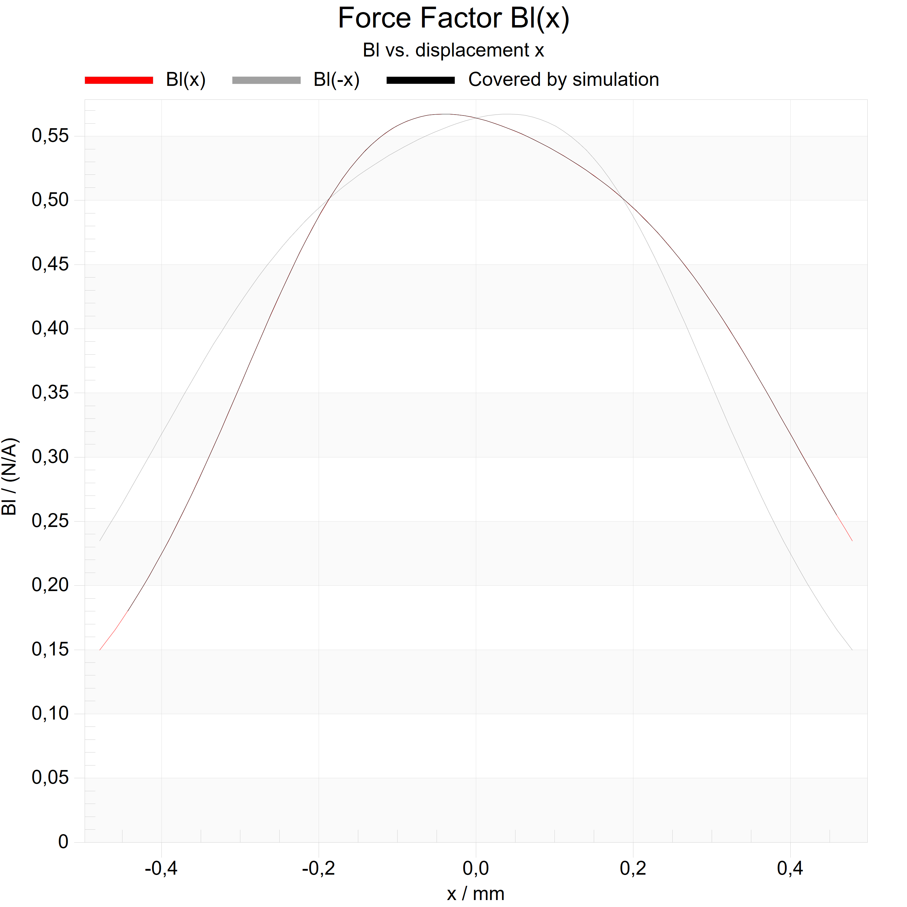
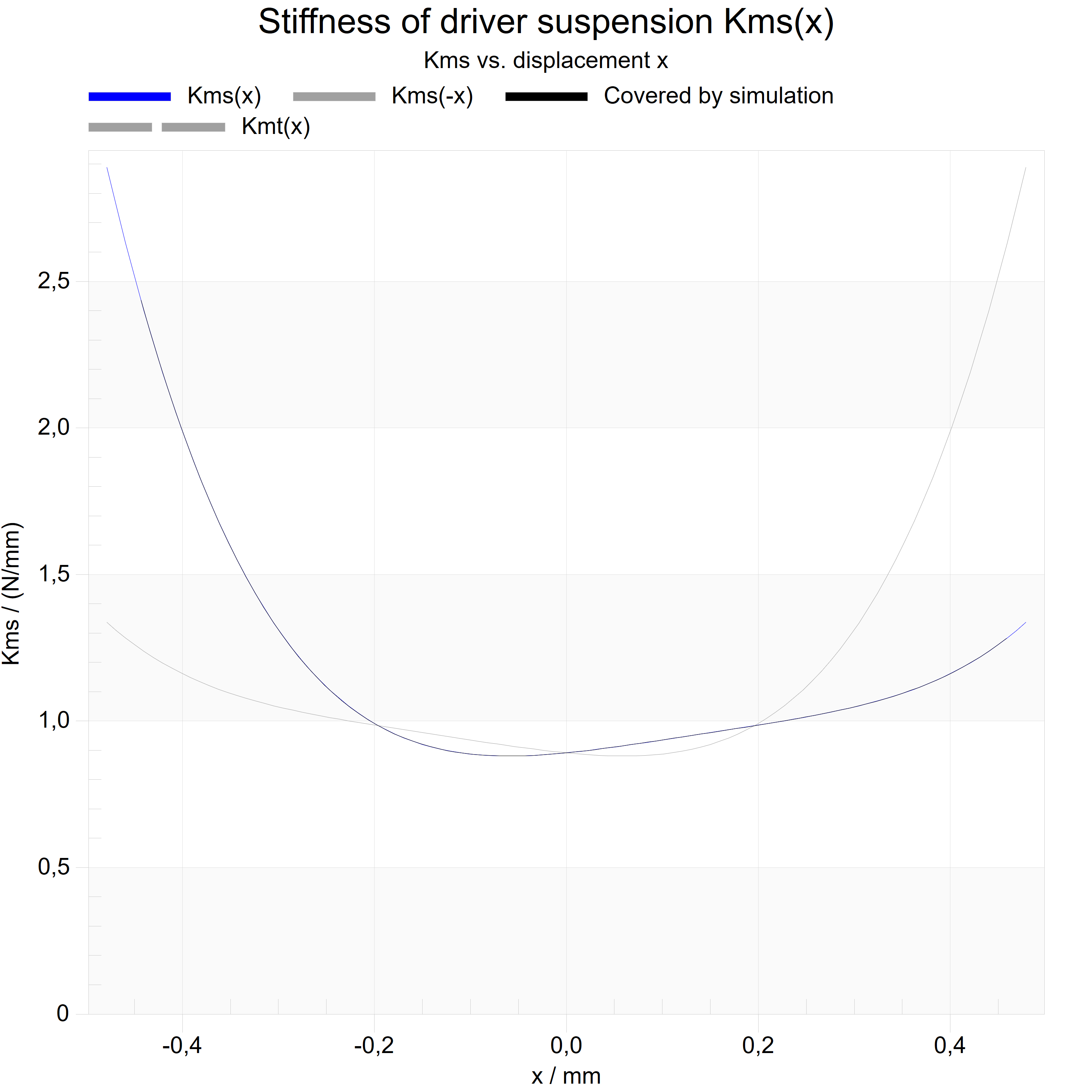
6. The windows Bl(x) and Kms(x) show the nonlinear characteristic of the force factor Bl and the stiffness K_ms versus displacement x, respectively. Black curves denote the range which was covered by simulation, colored curves represent the range identified by the LSI3 module.

   

SIM-AUR Simulation (time-lapse)

By using the Time-lapse Technique, the wait time until the simulation has finished can be greatly reduced. The reduction in simulation time depends on the so-called time-lapse factor r_tl. Higher numbers yield in faster simulation at the cost of precision. Changing the stimulus, the SIM‑AUR automatically sets a value representing a good compromise between speed and precision.

1. Open the folder Simulation, Auralization\Simulation Auralization (SIM‑AUR)\Simulation.

2. Open the object Microspeaker and double click the operation 2 SIM‑AUR Simulation (time‑lapse).

3. Inspecting the window Temperature, you will see the long-term temperature behavior. Since time-lapse is activated, the display differs from the Temperature window without time‑lapse technique:

   The dashed, grey curve shows the predicted magnet temperature ΔT_m over time, calculated using the time‑lapse technique. The solid curves ΔT_v (peak) and ΔT_m (mean) represent the solutions at so called calibration points, which are calculated solving the full loudspeaker model. Note that at those points there are significant changes in the level and/or spectral properties of the stimulus.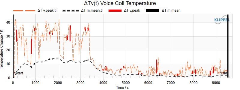

   

4. In the window Thermal Power Flow, you can also see the predicted dissipated powers using Time-lapse Technique vs. the precise solutions of the loudspeaker model.

   

SIM-AUR Auralization

1. Open the folder Simulation, Auralization\Simulation Auralization (SIM‑AUR)\Auralization.

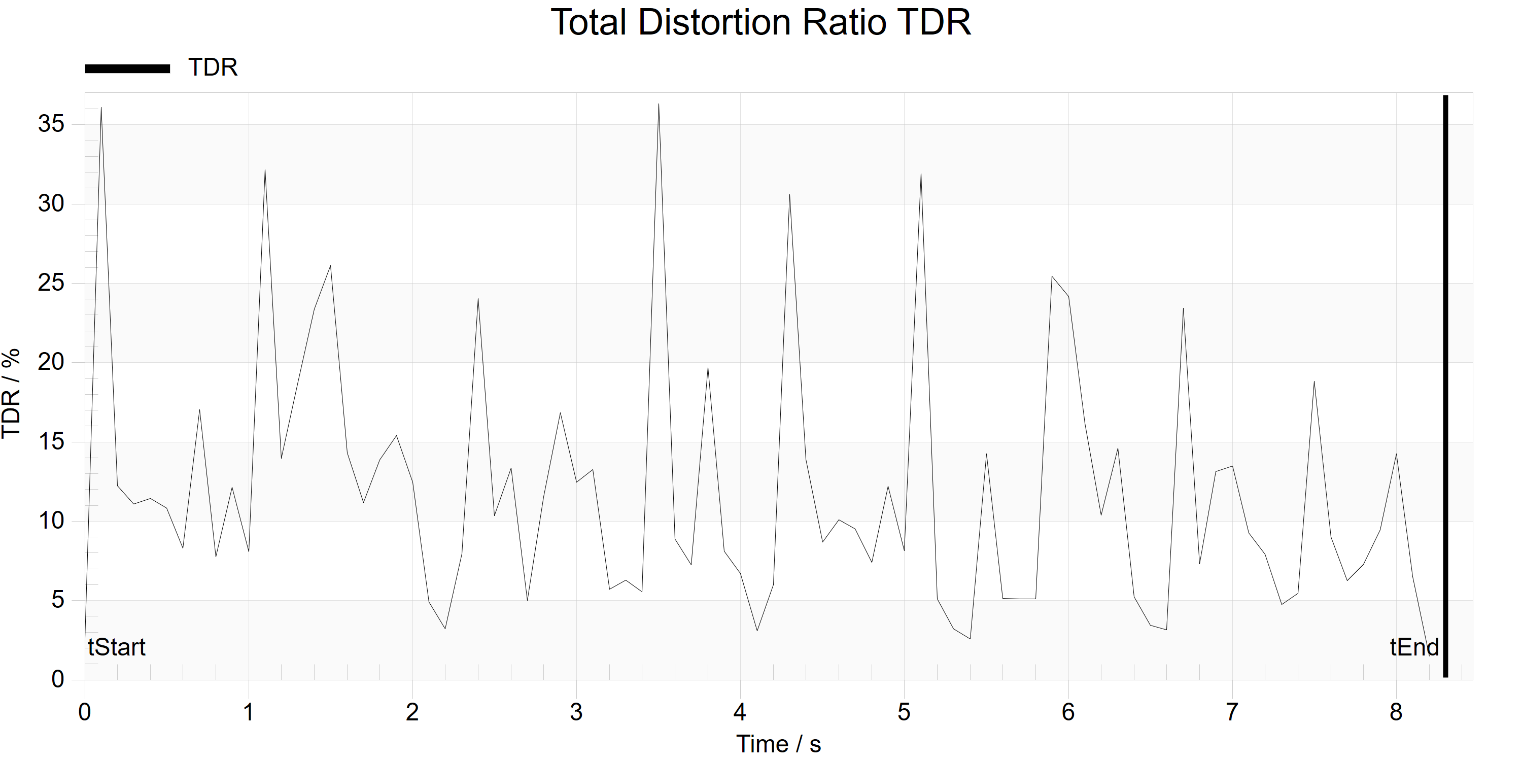
2. Open the object Microspeaker in Smartphone and double click the operation 3a SIM‑AUR Auralization.

3. The window Total Distortion Ratio shows you the peak distortion ratio of all distortions in the output signal in %.

   

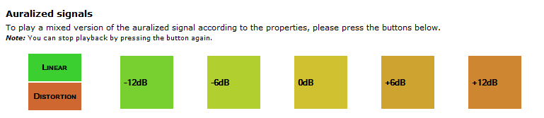
4. Using the buttons in the window Auralization, you can play a mixed signal of the pure linear and pure nonlinear signal. 0dB refers to the original scaled signal. You can change the mixing values at every time after a simulation was run.

   

5. Open the object Microspeaker in Smartphone and double click the operation 3b SIM‑AUR Auralization (prog. stiffness).

6. Take a look at the difference of the stiffness nonlinearity K_ms(x) – the curve was symmetrized virtually for the simulation (no new prototype). If you compare the windows TDR from both both operations, you will see that the total distortion ratio is significantly lower if the stiffness is symmetrized, since there is less 2^nd order distortion because of the symmetry.

   You’re welcome to compare the mixed signals of both operations, to hear the difference in symmetrizing the nonlinearity.

Performing a SIM-AUR Simulation (Part 2)

The second part of the tutorial is a step~by~step recipe to simulate and auralize a driver in the large signal domain. The SIM-AUR module needs the parameters of a real or conceptional driver. The tutorial uses the large signal parameters of one of your own drivers which you have already determined via the LSI Large Signal Identification module. As an alternative, you can use the driver data of the web example database.

Note

The nonlinear parameters can be conveniently transferred from the LSI or the SIM module to the SIM‑AUR module. To transfer the parameters, choose the property page “Im/Export” of the LSI or SIM module, and export the parameters to the clipboard. Afterward, import into the SIM‑AUR is possible. (see section Supported Modules for Im/Export)

Connect the Hardware

1. Connect a Klippel Dongle, Klippel Analyzer 3 (KA3) or Distortion Analyzer (DA) with the computer via USB.

2. Klippel Analyzer 3 (KA3) or Distortion Analyzer (DA): Connect power supply to measurement device.

SIM-AUR Simulation and Auralization

This section describes how a simulation is set up, and the results can be auralized based on the results. For a description to directly running an auralization, see SIM-AUR Auralization.

Simulation: Select Setup Parameter

1. Open or create a new database.

2. Click New Object and choose the Klippel template SIM-AUR Simulation Auralization.

3. Perform a Large Signal Identification (LSI or LSI3) operation to identify the large signal driver data.

4. Open the LSI operation, open the property page, navigate to the Im/Export tab and copy the results to the clipboard, by clicking Export to Clipboard.

5. OPTIONAL: Import the parameter to the SIM2-operation and perform a simulation to predict heating effects and check the maximum stimulus voltage.

6. Import the parameters in the operation SIM-AUR Simulation. Open the property page, navigate to the Im/Export tab and click Import from Clipboard.

7. Select a wav-file stimulus using the Path property in the category Stimulus.

8. Select a suitable input gain.

Note

In case of very high excitation levels the displacement x may exceed the range for which the nonlinear parameters are defined/measured for. The large signal parameters can differ widely from physics outside the defined/measured range. In case the displacement exceeds the defined range x_pse you will get a warning.

Activate the checkbox Show advanced and go to the category Transducer (nonlinear) to increase x_pse. Check the result page Model Parameters which show the nonlinear curves for the new x_pse range. If the parameters are still reasonable you can start the simulation again. If not, decrease the excitation level.

Simulation: Run Operation

Start the measurement by pressing the button Run or using the shortcut Ctrl+R.

To cancel the operation, use the button Abort . If the button Finish is shown result data is available and will be kept afterward.

Auralization: Select Setup Parameter

1. After performing a simulation, cursors are activated in all time-variant windows (such as Temperature, Power or Displacement). Using the cursors, you define a section which is auralized in the next step. To do so, either drag the cursors, or shift them to their position by using the shortcuts Shift + Left Click (sets start time) or Ctrl + Left Click (sets end time).

   Note

   Sections with a length up to 20 s are recommended.

2. Open the property page, and click the Button “Cut and Auralize” in the category “Measurement Setup”. A new operation is created, duplicating the setup of the auralization and allowing to auralize the chosen section in particular.

   The new operation will have the same name with an added “(section)” suffix.

   Note

   If the new operation is not shown, please click the button Refresh .

Auralization: Run Operation

Start the measurement by pressing the button Run or using the shortcut Ctrl+R.

To cancel the operation, use the button Abort . If the button Finish is shown result data is available and will be kept afterward.

SIM-AUR Auralization

In contrary to section SIM-AUR Simulation and Auralization, this section describes how an auralization can be performed without running a simulation first.

Select Setup Parameter

1. Open or create a new database.

2. Click New Object and choose the Klippel template SIM-AUR Simulation Auralization.

3. Perform a Large Signal Identification (LSI or LSI3) operation to identify the large signal driver data.

4. Open the LSI operation, open the property page, navigate to the Im/Export tab and copy the results to the clipboard, by clicking Export to Clipboard.

5. OPTIONAL: Import the parameter to the SIM2-operation and perform a simulation to predict heating effects and check the maximum stimulus voltage.

6. Import the parameters in the operation SIM-AUR Simulation. Open the property page, navigate to the Im/Export tab and click Import from Clipboard.

7. On the tab Setup in the category Measurement Setup, set the mode to Auralization.

8. Select a wav-file stimulus using the Path property in the category Stimulus.

9. Select a suitable input gain.

Note

In case of very high excitation levels the displacement x may exceed the range for which the nonlinear parameters are defined/measured for. The large signal parameters can differ widely from physics outside the defined/measured range. In case the displacement exceeds the defined range x_pse you will get a warning.

pse stands for power series expansion and defines the valid range of the power series to describe nonlinear parameter curves.

Activate the checkbox Show advanced and go to the category Transducer (nonlinear) to increase x_pse. Check the result page Model Parameters which show the nonlinear curves for the new x_pse range. If the parameters are still reasonable you can start the simulation again. If not, decrease the excitation level.

Run Operation

Start the measurement by pressing the button Run or using the shortcut Ctrl + R.

To cancel the operation, use the button Abort . If the button Finish is shown result data is available and will be kept afterward.

Auralization

After the operation was performed, open the window Auralization. You can listen to the auralized signals by pressing one of the displayed buttons. To stop the playback, press the same button again. To change the scaling, open the property page, go to the tab Setup, category Auralization and change the parameters S_dis (min) and S_dis (max).

SIM-AUR Reference

Overview

The SIM~AUR module performs a numerical simulation of either real or fictitious drivers based on a lumped parameter model. This reference provides a description of the separate operation types as well as a description of the used time-lapse and auralization technique.

For a detailed description of the used model, please refer to the SIM – Reference.

Theory

Thermal Simulation

The SIM-AUR module simulates the dynamic heating and cooling processes of the driver. Depending on the systems time constants and the excitation, the thermal system may not reach thermal equilibrium. The user can simplify the model by switching off the thermal resistances R_ta(x), R_tc(v), R_tt(v), R_tg, the thermal capacities C_tv, C_tg, and C_tm, and the direct heating due to eddy currents (α). This is useful if the corresponding thermal parameters are unknown.

Interaction between Thermal and Electro‑Mechanical Model

The thermal model is coupled to the electro-mechanical model by the state variables x, v, i, i₂, i₃ and the voice coil temperature T_v. The electro-mechanical model supplies the displacement x, the velocity v and the powers P_Re and P_eddy to the thermal model while the temperature increase ΔT_v is given back to the resistance R_e.

Coupling of thermal and electro-mechanical domain

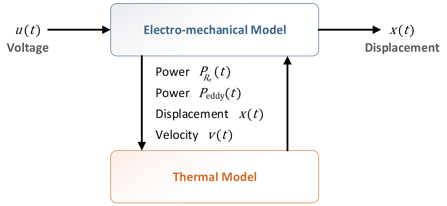
Formulas for interaction of thermal and electro-mechanical domain:

\[P_{R_{\text{e}}} = R_{e} \cdot i_{2}\]

\[P_{\text{eddy}} = R_{2} \cdot \left( i - i_{2} \right)^{2} + R_{3} \cdot \left( i - i_{3} \right)^{2}\]

Time-lapse Technique

For a fast prediction of the long term temperature response of the speaker, a simplified transducer model is used. To cope with the nonlinear performance of the speaker, the elements of the model are determined by solving the nonlinear model precise over a specific section T_cal.

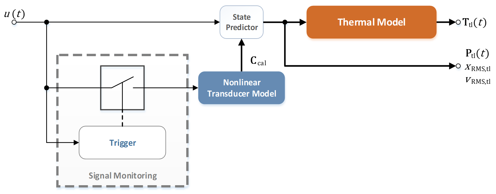
This process is therefore called „calibration“, depicted by the blue and red bars in the graphic above. Using the results of this precise simulation, simple elements are calculated, which comprises the nonlinear response of the transducer under the given excitation. Assuming relative slow variations in the spectral properties of the input signal, the temperatures can be predicted using these simplified elements. In case of change of the signal properties, the prediction may become invalid. To increase the prediction accuracy, multiple calibrations can be performed (depicted in red; additional calibration point).

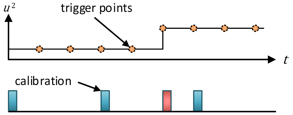
The simplified models are represented by four factors used to calculate the input of the thermal subsystem:

\[\begin{split}\mathbf{C}_{\text{cal}} = \begin{bmatrix}{\overline{Y}}_{\text{coil}} & {\overline{Y}}_{\text{eg}} & X_{\text{cal}} & V_{\text{cal}} \\\end{bmatrix}^{T}\end{split}\]

and defined by the equations:

\[{\overline{Y}}_{\text{coil}} = \left. \ \frac{{\overline{P}}_{\text{coil}}}{u_{\text{rms}}^{2}} \right|_{T_{\text{cal}}}\]

\[{\overline{Y}}_{\text{eg}} = \left. \ \frac{{\overline{P}}_{\text{eg}}}{u_{\text{rms}}^{2}} \right|_{T_{\text{cal}}}\]

\[X_{\text{cal}} = \left. \ \sqrt{\frac{x_{\text{rms}}^{2}}{u_{\text{rms}}^{2}}} \right|_{T_{\text{cal}}}\]

\[V_{\text{cal}} = \left. \ \sqrt{\frac{v_{\text{rms}}^{2}}{u_{\text{rms}}^{2}}} \right|_{T_{\text{cal}}}\]

Auralization

The SIM-AUR module offers an auralization feature based on separation of distinct nonlinear effects without modifying the internal states of the speaker model. The auralization is based on the precise nonlinear simulation of the transducer. Since all states z, which are used to describe the speaker at a distinct sample k, are known, nonlinear effects in each state variable can easily be separated using separation matrices. This technique gains the benefit of separating the nonlinear effects but not affecting the simulated speaker itself. The separated distortion signal p_dis can easily scaled using a linear gain S_dis.

u(t)

stimulus (input signal),

p_dis(t)

sound pressure of the nonlinear distortion

p_lin(t)

sound pressure of the linear signal

S_dis

linear gain factor for amplifying p_dis

p_aur(t)

auralized signal (output signal)

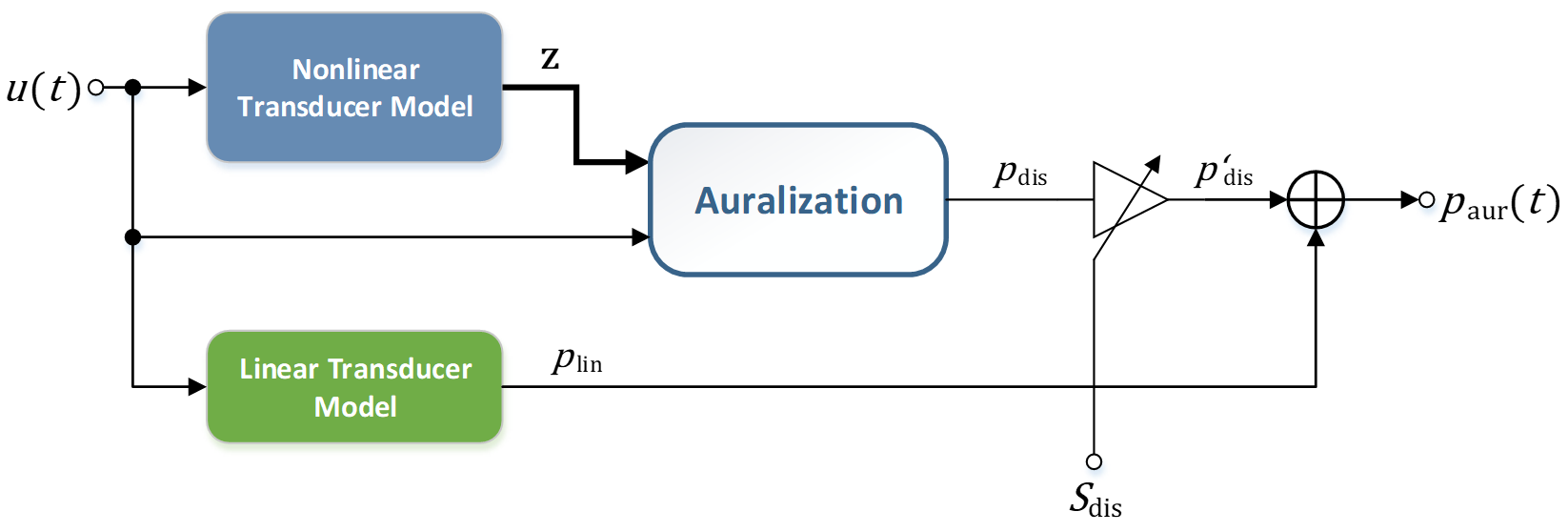
Flowchart of Auralization

Operations

How it Works

The SIM-AUR module uses transducer modelling to predict the system response in the target application. At first a long‑term simulation is performed, to predict the slow thermal state variables as the speaker is driven in the target application. Based on this data, a precise simulation of a section can be performed, yielding in precise simulation data for state variables such as displacement x and the total distortion ratio TDR. Afterward, the distortion signal of the section can be separated and auralized, to evaluate the performance using perceptive modelling or listening tests.

Sequence steps for Auralization

In contrary to other modules, SIM-AUR operations maybe based on each other. Thus, you can first simulate the long‑term behavior of the transducer, simulate afterward distinct sections and auralize the transducer. A typical workflow is shown in the picture below.

Operation Modes

Simulation

The “Simulation”-mode is used to determine the long term performance of the transducer. In respect to the states of the electro-mechanical system, thermal states are changing relative slow (time constant of the magnet might be about ~1.5h). To speed up the prediction of the thermal states, a Time-lapse Technique can be used. The predicted temperatures can reveal section of great interest (e.g. sudden changes in the signal energy).

Please note (as stated above) that a simulation using Time-lapse Technique will only produce precise solutions on special points. Thus, if you are interested in the full long-time behavior, you may avoid the Time-lapse Technique.

After a simulation, you can use the cursors in windows with time dependency to define a section for auralization.

Auralization

The “Auralization”-mode can be used to auralize the simulated transducer. After performing the auralization, you can listen to the predicted sound pressure and virtually in- or decrease the distortions of the transducer via a very simple mixing console.

If you want to change the possible gain factors of the distortion part S_dis, no new auralization has to be performed.

Same as in the “Simulation”-mode, you can specify a more interesting region by placing the cursors and simulate afterwards.

Note

If you are using the mode „Simulation“, and activate the time‑lapse feature, certain information is not available (e.g. the State Variable window, R_e(t) window and others). This is due to the fact that time-lapse simulation does not offer prediction of the state variables over the complete signal, but only on certain trigger points (see above).

Property Page

After activating a SIM~AUR operation you can open the property page. Every setup parameter is located in the property page “Setup” and sorted in different categories.

Note

The shown categories and available parameters are depending on the operation type. Advanced options are hidden by default.

Basic

Measurement Setup

Mode

Mode: Simulation: Perform a simulation of the loudspeaker model. For a faster simulation of long signals,

the time‑lapse feature is available.; Auralization: Separates the distortion signal generated by the loudspeaker

nonlinearities from the complete signal. The separated signals may be used for further investigation, or for creating

listening tests.

Specifies the mode of the SIM‑AUR. Available Modes:

Solver

The solver for the numerical solution of the system equations can be chosen by the user. If Fast Solver is selected, a solver without step size control will be used. This solver is very fast and will calculate in most cases the exact speaker states. In some few cases the precision will suffer and a more sophisticated solver with step size control has to be used (Precise Solver).

Stimulus

Path

Absolute path to the location of the excitation stimulus.

Stimulus Length

[Read Only] Length of the stimulus.

Channels

[Read Only] Number of stimulus file channels.

Sample Rate

[Read Only] Sampling frequency of the stimulus.

Used Channel

Used channel of the excitation stimulus. Only available if wav‑file has more than one channel.

Input Gain

Linear gain applied to the voltage signal on the speaker terminals. It is assumed that the digital “1” of the wav‑file corresponds to 1 V.

Time‑lapse Factor

If activated, the thermal operation is performed using the Time-lapse Technique. Certain windows may not be available if activated.

The time‑lapse factor is stimulus length specific. Valid values are calculated by the SIM‑AUR and made

available as a list. A reasonable time‑lapse factor is set automatically.

If time‑lapse cannot be performed, the property is not displayed.

Note

Only available for Simulation mode

Initial Parameters

Voice Coil Displacement

Voice coil displacement \(x_{t=0}\). This value can be used to trigger instabilities such as bifurcation effects when selecting positive or negative initial values.

Auralization

This category is only available for the “Auralization” mode.

S_dis (min)

Minimum value of the scaling factor of the nonlinearities S_dis in dB.

This parameter defines the lower limit of the available S_dis-values for the auralization.

S_dis (max)

Maximum value of the scaling factor of the nonlinearities S_dis in dB.

This parameter defines the upper limit of the available S_dis-values for the auralization.

S_dis (min)

Step width Δs (in dB) which is used to generate the vector. The algorithm will always set the last value to \(S_{\text{dis,max}}\).

\[\begin{split}S_{\text{dis}} = \begin{bmatrix} S_{\text{dis,min}} & S_{\text{dis,min}} + \mathrm{\Delta}s & \cdots & S_{\text{dis,max}} \\\end{bmatrix}\end{split}\]

Display

State Signal

Determines the signal (speaker state) for which the results are to be shown. Depending on the selected enclosure, you can choose one of the following parameters:

- x (cone displacement),

- v (cone velocity),

- i (input current),

- p_box (pressure in box),q_r (volume velocity of passive radiator),

- x_r (displacement of passive radiator),

- q_p (volume velocity of port),

- p_front (sound pressure in front enclosure),

- q (radiated volume velocity),

- p_far (far‑field sound pressure)

Obviously, some signals are only available if the correct enclosure was selected:

- p_box is only available if the driver is not mounted in a baffle

- q_r and x_r are only available for a passive radiator

p_front is only available for bandpass/sidefire systems

Transducer

The Transducer Property Page is visibly only, if the Show advanced Options on property page Basic setting is enabled.

Driver

S_d

Effective projected surface area of the driver diaphragm

d_d

Diameter of round effective radiation surface

Electrical Transducer Parameters

R_e

Electrical voice coil resistance at DC

Inductance Model

Different inductance models can be used for simulation.

The simplest model is the Single Inductance where the inductance is modeled by \(Z(s) = s \cdot L_{\text{e}}\) .

The LR-2 is a more complex models. The inductance is modeled by \(Z(s) = s \cdot L_{\text{e}} + s \cdot L_{2} || R_{2}\)

L_e

Voice coil inductance

R₂

Electric resistance due to eddy current losses

L₂

Electrical inductance due to eddy current losses

Note

LR-3 modeling in the simulation is not supported.

Mechanical Transducer Parameters

Bl

Effective instantaneous electrodynamic coupling factor (force factor of the motor) defined by the integral of the magnetic flux density B over the voice coil length l

K_ms

Mechanical stiffness of driver suspension

R_ms

Mechanical resistance of driver suspension losses

M_ms

Mechanical mass of driver diaphragm assembly including voice coil and air load

f_s

[Read Only] Transducer resonance frequency

Q_ms

[Read Only] Mechanical Q-factor considering Rms only

Q_es

[Read Only] Electrical Q-factor

Q_ts

[Read Only] Total Q-factor

Active Transducer Nonlinearities

Select the active transducer nonlinearities for the simulation. You can select the following nonlinearities:

• Bl(x), Bl(i)

• L_e(x), L_e(i)

• K_ms(x)

• R_ms(v)

• R₂(x), L₂(x)

• S_d(x)

• Reluctance Force

• Doppler Distortion

[EDIT] Nonlinear Parameters

This category is only available if at least one editable nonlinearity is set active.

Nonlinearity

Select nonlinearity for parameter editing.

Range

Specify the validity range for all nonlinearities depending on this signal.

On import from a Large Signal Identification (LSI) module, this is set automatically to the working range.

Warning

Caution: If you change this parameter, make sure that the nonlinear curves look reasonable!

Shift

Linear shift of the power series.

The shift can be used to e.g. simulate different voice coil offsets.

Order

Order of the power series.

Higher orders may yield better results for complex nonlinearity shapes in the validity region as specified by

Range, but may be completely off outside!

c₁ … c₈

Coefficients of a regular power series, used to describe the nonlinearity.

System

The System Property Page is visibly only, if the Show advanced Options on property page Basic setting is enabled.

Enclosure

System Type

Range: Driver in Baffle; Closed Box; Vented Box; Passive Radiator; Bandpass/Sidefire

Specifies the type of enclosure, in which the driver is supposed to be mounted. The type of the chosen enclosure will affect the overall system behavior (as opposed to simple transfer functions). Available Enclosure types:

Leaky Box

If active, it is assumed that the simulated enclosure contains additional losses introduced by leaks.

V_b

Volume of air in enclosure

V_f

Volume of air in front enclosure

R_ap

Acoustic resistance of port losses

M_ap

Acoustic mass of port including air load

R_ap

Acoustic resistance of port losses

M_mr

Mechanical mass of passive radiator diaphragm including voice coil and air load

R_mr

Mechanical resistance of passive radiator suspension losses

K_mr

Mechanical stiffness of passive radiator suspension

S_p

Surface area of port

S_r

Effective projected surface area of passive radiator diaphragm

f_c

[Read Only] Resonance frequency of the closed box system (Closed box only)

f_b

[Read Only] Resonance frequency of enclosure-port system

f_f

[Read Only] Resonance frequency of enclosure-port system (Bandpass/Sidefire only)

Q_tc

[Read Only] Q-factor of the closed box system (considering system load)

Q_p

[Read Only] Q-factor considering port losses

Cone, Radiation, Room

Radiation Model

Specifies how the sound pressure in the far field is calculated. You can choose between:

- Piston / 2pi / anechoic

Simulates the far field sound pressure in a half space environment.

- Piston / 4pi / anechoic

- Simulates the far field sound pressure in a full space environment.

Radiation Distance

On‑axis distance to the radiated point in the far-field

Active System Nonlinearities

Select the active system nonlinearities for the simulation. Depending on the selected enclosure, the following nonlinearities can be selected:

• R_al(p_box)

• K_ab(p_box)

• R_ap(v_p)

• K_mr(x_r)

• K_f(p_front)

• K_f(x)

[EDIT] Nonlinear Parameters

This category is only available if at least one editable nonlinearity is set active.

Nonlinearity

Select nonlinearity for parameter editing.

Range

Specify the validity range for all nonlinearities depending on this signal.

On import from a LSI – Large Signal Identification module, this is set automatically to the working range.

Warning

Caution: If you change this parameter, make sure that the nonlinear curves look reasonable!

Shift

Linear shift of the power series.

The shift can be used to e.g. simulate different voice coil offsets.

Order

Order of the power series.

Higher orders may yield better results for complex nonlinearity shapes in the validity region as specified by

Range, but may be completely off outside!

c₁ … c₈

Coefficients of a regular power series, used to describe the nonlinearity.

Thermal

The Thermal Property Page is visibly only, if the Show advanced Options on property page Basic setting is enabled.

Thermal Parameters

Voice Coil Material

Range: copper; aluminium; custom

Material of the voice coil wire. Available options are:

Temperature Coefficient

User-definable first order temperature coefficient of the voice-coil material

R_tv

Thermal resistance of path from voice-coil to pole tips and magnet surface

R_tg

Thermal resistance of path from pole tips to magnet and frame

R_tm

Thermal resistance of path from magnet to ambient air

α

Distribution of heat caused by eddy currents on voice-coil and magnet

r_v

Convection cooling parameter describing the dependence of R_tc from cone velocity

r_x

Convection cooling parameter describing the dependence of R_ta from cone displacement

r_b

Convection cooling parameter describing the dependence of R_tt from cone velocity

C_tv

Thermal capacitance of voice-coil and voice-coil former

C_tg

Thermal capacitance of pole tips and magnet surface close to voice-coil

C_tm

Thermal capacitance of magnet and frame

Approximate C_tg

Use an C_tg approximation derived from the given parameters

Result Windows

u(t) Voltage, i(t) Current

This result window shows the voltage at the speaker terminals u as well as the input current i over the measurement time t.

x(t) Displacement

Depending on the mode, the window shows the maximum absolute values of

• the displacement signal (precise solutions) x (max absolute),

• the distortion part of the displacement signal x_dis (max absolute) [auralization only],

• the effective displacement x (RMS), and

• the effective predicted displacement x (RMS, time-lapse) [time‑lapse only]

over time t.

v(t) Velocity

The window shows the predicted effective velocity of the time-lapse solver as well as the precise solutions of the calibrator.

Depending on the mode, the window shows the maximum absolute values of

• the velocity signal (precise solutions) v (max absolute),

• the distortion part of the velocity signal v_dis (max absolute) [auralization only],

• the effective velocity v (RMS), and

• the effective predicted velocity v (RMS, time-lapse) [time‑lapse only]

over time t.

ΔTv(t) Temperature

Depending on the thermal model and the simulation mode, this window shows the mean and peak values of

• the predicted voice-coil difference temperature Delta Tv,

• the predicted pole-tip difference temperature Delta Tg,

• the predicted magnet difference temperature Delta Tm,

over time t.

Note

In the mode “Simulation” with activated time-lapse, all curves are also shown as predicted curves using the time-lapse feature.

P(t) Input Power

This window displays the predicted input power P_Re which represents the power that goes directly into the voice coil and heats up the driver over time t.

Note

In the mode “Simulation” with activated time-lapse, all curves are also shown as predicted curves using the time-lapse feature.

Thermal Power Flow

This window gives an insight in the power flows of the thermal model over the time t. It shows the mean and peak values of dissipated and transferred powers P_coil, P_eg, P_con, P_dTv and P_g.

Note

In the mode “SIM-AUR Simulation” with activated time-lapse, all curves are also shown as predicted curves using the time-lapse feature.

Bypass factor

The result window shows the bypass factor γ over the measurement time t. The bypass factor describes the contribution of the input power, which bypasses the thermal resistance R_tv. A high bypass factor can be interpreted as a high amount of convection cooling due driver excitation. It is defined by

\[\gamma\left( t \right) = \frac{P_{\text{con}}\left( t \right) + P_{\text{eg}}\left( t \right)} {P_{\text{con}}\left( t \right) + P_{\text{eg}}\left( t \right) + P_{\text{tv}}\left( t \right)}\]

Re(t) Resistance

The result window shows the DC resistance of the voice-coil versus the measurement time t. The thermal dependence of the resistance is defined by

\[R_{\text{e}}\left( T_{\text{v}} \right) = R_{\text{e}} \cdot \left( 1 + \delta \cdot \mathrm{\Delta}T_{\text{v}} \right)\]

Note

This window is not available if the time-lapse feature is activated.

TDR(t) Total Distortion Ratio

The window shows the total distortion ration TDR of the radiated sound pressure p_far versus the measurement time t. The total distortion ratio is defined by

\[TDR\left( t \right) = \frac{\max_\limits{T}\left| p_{\text{dis}}\left( t \right) \right|} {\max_\limits{T}\left| p_{\text{lin}}\left( t \right) + p_{\text{dis}}\left( t \right) \right|} \cdot 100\%\]

where

\[p_{\text{far}}\left( t \right) = p_{\text{lin}}\left( t \right) + p_{\text{dis}}\left( t \right)\]

SPL(t) Sound Pressure Level

This window shows the predicted radiated sound pressure level of the transducer over time t. If run in mode “Auralization”, also the peak distortion part of the sound pressure Peak Distortion SPL is available if a nonlinear simulation is performed.

Note

This window is not available if the time-lapse feature is activated.

State Variable

The result window shows the peak, bottom, DC as well as the RMS value of one state variable of the state vector z of the electro-mechanic-acoustical system versus measurement time t.

The displayed state variable can be changed using the property State variable in the category Display.

Note

This window is not available if the time-lapse feature is activated.

Distortion Ratio

The window shows the ratio of one nonlinear distortion variable and its corresponding state variable of the electro-mechanic-acoustical system versus measurement time t. It is defined by

\[DR\left( t \right) = \frac{\max_\limits{T}\left| \mathbf{z}_{\text{dis}}\left( t \right) \right|} {\max_\limits{T}\left| \mathbf{z}_{\text{lin}}\left( t \right) + \mathbf{z}_{\text{dis}}\left( t \right) \right|} \cdot 100\%\]

The shown state variable can be changed using the property State variable in the category Display.

Crest Factor

The crest factor shows the ratio of the peak to the effective value. A high crest factor indicates that the signal includes extreme peaks, whereas a crest factor of 1 indicates direct current. It is defined by

\[d_{\text{crest}}\left( t \right) = \frac{\max_\limits{T}\left| \mathbf{z}\left( t \right) \right|}{\left. \ \mathbf{z}_{\text{RMS}} \right|_{T}}\]

Table Model Parameters

This window displays information of the nonlinear parameters as well as Thiele/Small parameters, thermal parameters and enclosure parameters.

Auralization

After auralization, this window shows a simple mixing console which you can use to listen to the auralized signal. By clicking the buttons the mixed auralized the far-field sound pressure p_aur with

\[p_{\text{aur}}\left( t \right) = p_{\text{lin}}\left( t \right) + S_{\text{dis}} \cdot p_{\text{dis}}\left( t \right)\]

can be heard. The mixing depends on the chosen values S_dis,min, S_dis,max and Step width of S_dis. Changing these parameters will update the result page, no additional auralization must be performed.

This output page can be exported using the “Export”-button and inspected in every web-browser.

Note

This window is not available if the time-lapse feature is activated.

Bl(x) Force Factor

The nonlinear force factor characteristic Bl(x) is displayed versus displacement x. The gray line shows the force factor mirrored at the rest position. It is useful to assess the curve asymmetry at a glance. The black line (visible after completing simulation) indicates the part of the characteristics that was used for the simulation.

Kms(x) Stiffness

The nonlinear stiffness characteristic K_ms(x) is displayed versus displacement x. The gray line shows the stiffness mirrored at the rest position. It is useful to assess the curve asymmetry at a glance. The black line (visible after completing simulation) indicates the part of the characteristics that was used for the simulation.

If the enclosure model is set to “closed box”, an additional stiffness curve K_mt(x) is shown, representing the combined stiffness of driver suspension and box

\[K_{\text{mt}}\left( x \right) = K_{\text{ms}}\left( x \right) + \frac{1}{C_{\text{ab}}\left( 0 \right)}\]

Le(x) Inductance

The nonlinear inductance characteristic L_e(x) is displayed versus displacement x. The black line (visible after completing simulation) indicates the part of the characteristics that was used for the simulation.

Le(i) Inductance

The nonlinear inductance characteristic L_e(x=0,i) is displayed versus current i. The black line (visible after completing simulation) indicates the part of the characteristics that was used for the simulation.

L2(x) Para‑Inductance

The nonlinear voice coil para-inductance L₂(x)is plotted versus cone displacement *x. Note that the curve is shown only if an appropriate inductance model is selected in the category Transducer. The black lines (visible after completing simulation) indicate the part of the characteristics that was used for the simulation.

R2(x) Resistance

The nonlinear electrical resistance R₂(x)* due to eddy current losses is plotted versus cone displacement x. Note that the curve is shown only if an appropriate inductance model is selected in the category Transducer. The black lines (visible after completing simulation) indicate the part of the characteristics that was used for the simulation.

Rms(v) Mechanical Resistance

The nonlinear resistance characteristic R_ms(v) is displayed versus velocity v. The gray line shows the resistance mirrored at the rest position. It is useful to assess the curve asymmetry at a glance. The black line (visible after completing simulation) indicates the part of the characteristics that was used for the simulation.

Ral(p) Acoustical Leakage Resistance

The nonlinear acoustical resistance of leakage losses characteristic R_al(p_box) is displayed versus sound pressure in box enclosure p_box. The gray line shows the acoustical resistance mirrored at the rest position. It is useful to assess the curve asymmetry at a glance. The black line (visible after completing simulation) indicates the part of the characteristics that was used for the simulation.

Rap(v) Acoustical Port Resistance

The nonlinear acoustic resistance R_ap(v_p) of the vent losses is displayed versus velocity vp of the port. The gray line shows the resistance mirrored at the rest position. It is useful to assess the curve asymmetry at a glance. The black line (visible after completing simulation) indicates the part of the characteristics that was used for the simulation.

Kmr(x) Passive Radiator Stiffness

The nonlinear stiffness characteristic K_mr(x_r) of passive radiator suspension system is displayed versus passive radiator displacement x_r. The gray line shows the stiffness mirrored at the rest position. It is useful to assess the curve asymmetry at a glance. The black line (visible after completing simulation) indicates the part of the characteristics that was used for the simulation.

Sd(x) Radiating Surface Area

The nonlinear effective relative radiating surface characteristic S_d(x) is displayed versus displacement x. The gray line shows the effective relative radiating surface mirrored at the rest position. It is useful to assess the curve asymmetry at a glance. The black line (visible after completing simulation) indicates the part of the characteristics that was used for the simulation.

Note

This is a relative curve, meaning that the effective radiating surface characteristic can be obtained by multiplying the curve by S_d.

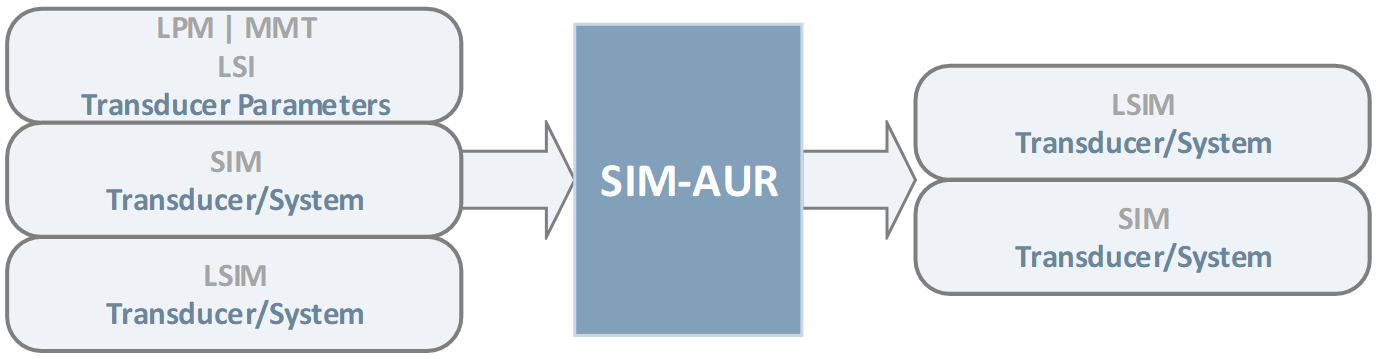
Supported Modules for Im/Export

Malfunction and Troubleshooting

Overview

This chapter will provide information that can help you solve common problems that occur with the SIM module. The software generates a variety of warnings automatically if the signals are badly conditioned or a malfunction state is detected. Some information may be neglected but it is always recommended to find out the cause of the problem.

If you cannot find a description here that matches your problem, try these options:

• Check the Malfunction and Troubleshooting section of the SIM Simulation 2.0 documentation.

• Check the Malfunction and Troubleshooting section of the dB-Lab documentation.

• support.

Error and Warning Messages

Primary data is already available

Cause: Simulation results will be deleted if the corresponding setup parameter are changed. This way results and setup parameter are kept consistent. If you want to perform a new simulation while preserving the old results, please create a new operation.

Remedy:

• Duplicate the operation, using Edit – Duplicate, or pressing the duplicate button .

• The setup parameters of the old simulation can be conveniently copied to new operation with the Copy and Paste buttons that you find on property page Im/Export (see above).

Driver model could not be solved

Cause: For certain combinations of model parameter values the driver model becomes very stiff. This is particular true for large voice coil displacements. The stiffer the model is the more it obstructs numerical simulation. The reason for stiffness are dynamic modes with time constants that differ by a factor of 1000 or more. Although a special solver for stiff models is implemented the simulation may fail for very stiff models. Note that any numerical simulation algorithm may fail to converge. Normally a divergence can easily be detected as meaningless results are produced.

Remedy:

• Try another solver. Per default, a Fast Solver.

  Activate checkbox Show advanced and change the solver type to Precise solver.

• Change the model parameters slightly. Especially increase the values of L₂, R₂, L_e and K_ms if they are very small. Slight changes of the model parameters will normally a negligible impact on the simulation results but may reduce stiffness considerably.

• Deactivate the L_e(i) nonlinearity.

• Decrease the Input Gain (see category Stimulus).

Driver model could not be solved

Cause: For certain combinations of model parameter values the driver model becomes very stiff. This is particular true for large voice coil displacements. The stiffer the model is the more it obstructs numerical simulation. The reason for stiffness are dynamic modes with time constants that differ by a factor of 1000 or more. Although a special solver for stiff models is implemented the simulation may fail for very stiff models. Note that any numerical simulation algorithm may fail to converge. Normally a divergence can easily be detected as meaningless results are produced.

Remedy:

• Try another solver. Per default, a Fast Solver.

  Activate checkbox Show advanced and change the solver type to Precise solver.

• Change the model parameters slightly. Especially increase the values of L₂, R₂, L_e and K_ms if they are very small. Slight changes of the model parameters will normally a negligible impact on the simulation results but may reduce stiffness considerably.

• Deactivate the L_e(i) nonlinearity.

• Decrease the Input Gain (see category Stimulus).

Warning

Displacement exceeded approved range

Cause: The peak displacement achieved during the simulation exceeded than the displacement range Xpse for which the power series of the nonlinearities Bl(x), K_ms(x) and L_e(x) are defined. The power series may behave quite differently outside the “approved” range x = ± Xpse.

Remedy: Decrease excitation level in order to simulate inside the “approved” range. If you want to simulate with this high excitation go to category Transducer (nonlinear), set Nonlinearity to Bl(x) and increase Xpse. Check the result windows Bl(x), Kms(x) and Le(x). Do the nonlinear parameters look reasonable for the increased displacement range?

Warning

Port velocity exceeded approved range

Cause: The peak velocity in the port achieved during the simulation exceeded than the velocity range Vp pse for which the power series R_ap(v_p) is defined. The power series may behave quite differently outside the “approved” range v_p = ± Vp pse.

Remedy: Decrease excitation level in order to simulate inside the “approved” range. If you want to simulate with this high excitation go to category System (nonlinear), set Nonlinearity to R_ap(v_p) increase Vp pse. Check the result windows Rap(Vp). Looks R_ap(v_p) reasonable for the increased velocity range?

Further problems

Simulation results are widely off

In case of very high excitation levels the displacement x (or the air velocity v_p in port) may exceed the range for which the nonlinear parameters are defined/measured for. The large signal parameters can differ widely from physics outside the defined/measured range and the simulation will fail badly.

Check the result windows Bl(x), Kms(x), Le(x) and Rap(Vp). The x-axis of the plots are adjusted to range covered by x and v_p during the simulation. Do the large signal parameters look reasonably for this range? If not, decrease the excitation level.

Note

It is always recommended to perform a simulation using the SIM Simulation 2.0 module first and check if the results look meaningful. This helps to find problems with the simulation before running long term simulations, which may take a significant amount of time.