MPM – Material Parameter Measurement

Overview

What is MPM?

The Material Parameter Measurement (MPM) measures the Young’s modulus \(E\) and loss factor \(\eta\) of materials used for loudspeaker parts at a certain modal frequency and temperature. It is a dynamic technique which excites a defined material beam pneumatically under similar conditions as operated in a loudspeaker driver.

The measurement method is applicable to all materials and is simple to handle. It is touchless, nondestructive and robust.

Putting into Operation

Overview

Step-by-step instructions are provided to setup the hardware of the Material Parameter Measurement System for the first time. It is assumed that a Suspension Part Measurement bench (SPM) from KLIPPEL is available and installed. Furthermore, the Distortion Analyzer Hardware and dB-Lab software as well as the TRF module are installed.

Please find additional instructions for installing the dB-Lab software and general information to the measurement hardware in other parts of the manual dedicated to dB-Lab, Hardware, TRF-Module.

Setting up the System

The setup uses the following hardware components:

• Measurement bench for pneumatic excitation of the suspension part (SPM)

• MPM clamping set

• Distortion Analyzer (DA2) or Klippel Analyzer 3 (KA3) hardware [1]

• Amplifier + XLR cable

• Amplifier cable with Speakon connector

• SPM Speaker cable (extra-long with two Speakon connectors)

• Laser displacement sensor

• Microphone

and software components:

• Transfer Function Module (TRF)

• Material Parameter Software [2]

[1]

The Material Parameter Measurement supports both Distortion Analyzer as well as Klippel Analyzer 3 hardware. For more information regarding the setup of your specific system, please look in the Hardware Manual. If you are measuring with the KA3, please also attach the supplied Dongle.

[2]

The application “MPM Automatic” is delivered as separate .exe.

Step 1: MPM Clamping Set

Step 1.1: MPM Clamping Set Overview

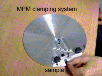
The MPM provides a special clamping set which comprises:

Number	Units	Parts
1	1	platform
2	1	adjustment tool
3	1	clamping beam
4	2	threaded bolts

The adjustment tool allows clamping the material samples as a beam of defined length performing the first bending mode.

Step 1.2: Define the beam length

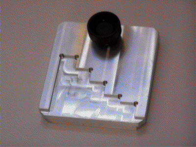
The adjustment tool comprises for slots having a length of 15, 20, 30, 40 and 50 mm.

Step 2: Mounting Instruction SPM Bench

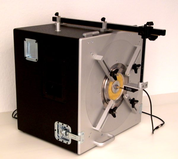
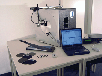
The MPM can be used with the SPM measurement box or smaller LST bench for the pneumatic excitation. Below you find a detailed description how to setup MPM hardware in both configurations. There is a movie available at www.klippel.de showing the setup and handling of the MPM in practice.

Step 2.1: SPM measurement bench overview

Step 2.2: Install MPM platform

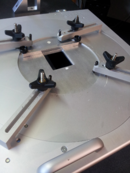
• Open the SPM box and bring door in horizontal position

• Loosen the turnbuckles to release horizontal position

• Remove all rings used for clamping suspension parts.

• Remove the guiding rod.

• Insert MPM platform in hole of door and fix it with levers.

Step 2.3: Mount the Laser

• Close the door of the SPM box to bring MPM clamping platform in vertical position.

• Mount the laser.

Step 2.4: Insert the Microphone

• Cut a small hole in the rubber plug that covers the microphone mounting plate. (Two crossed cuts are favorable to fit with the microphone. If the microphone is not mounted (for SPM measurements) the hole can be closed with a microphone dummy (pencil) or with tape to avoid air noise.)

• Insert the microphone into the box.

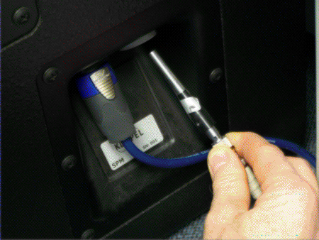
• Connect Speaker 1 output of the measurement device with loudspeaker terminal in the SPM box.

Step 3: Mounting Instruction LST bench

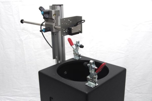
Step 3.1: Put the LST measurement bench in vertical position

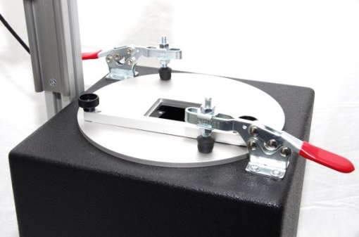
Step 3.2: Mount the MPM clamping to the LST bench

Step 3.3: Put the LST bench in horizontal position and adjust the laser to the DUT

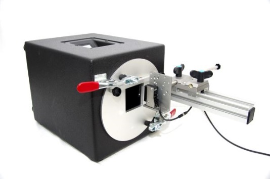
Step 4: Cables and Connections Overview

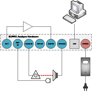
Connect the components in the following way:

1. The output OUT1 of the measurement device provides the stimulus signal and is connected with the input of the power amplifier.

2. The output of the power amplifier is connected with the Speakon connector AMP at the rear side of the measurement device.

3. The laser displacement sensor is connected with the laser connector at the measurement device.

4. The output SPEAKER 1 of the measurement device is connected with the working bench by using the special SPM speaker cable.

5. Usually you can connect the microphone into the IEPE port of the measurement device.

MPM - Tutorial

What is the goal of these tutorials?

The following tutorials give a step-by-step instructions how to use the Material Parameter Measurement (MPM).

• The Tutorial 1 – Viewing Results interprets the results of the MPM.

• The Tutorial 2 – Performing a measurement describes how to measure your own material part.

• The Tutorial 3 – Customizing MPM provides tips how to get the most out of MPM.

Tutorial 1 – Viewing Results

The results of the measurement are stored in two ways:

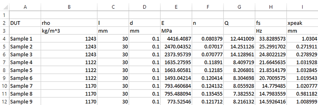
1. The most important results are usually stored in a .txt file called summary.txt located in the folder where all the results of one measurement series are collected. This file can be viewed by a simple text editor or exported to any table oriented post processing software (e.g. EXCEL \(^{©}\)) as shown below.

2. The details of each single measurement are stored in a database NAME.kdbx which corresponds with the NAME of the material sample. The detailed inspection of the measured responses and the calculated material parameters is recommended for setting up the system, checking the performance of the sensors (microphone and laser) and for finding the causes of any malfunction.

Viewing database with dB-Lab

An example of the content of a NAME.kdbx file is provided in the Example Database located in your KLIPPEL application data folder for RnD. Click on this file to activate dB-Lab which is the frame software of the KLIPPEL R&D system to view the detailed data of this particular measurement.

Open the Transducer Part + Material (SPM, MSPM, LST, BFS, MPM) folder using the Open folder content button. Then select the driver MPM (Automatic).

dB-Lab shows the driver MPM (Automatic) which comprises a collection of four operations as shown below.

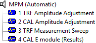
The first measurement 1 TRF Amplitude Adjustment and the following mathematical post processing operation 2 CAL Amplitude Adjustment are used to adjust the amplitude of the stimulus. If the measured peak displacement at the resonance frequency is approximately equal to the target displacement defined by the user the main measurement 3 TRF Measurement Sweep will be performed and the measured transfer function between sound pressure in the box and displacement of the beam is calculated. After transferring this transfer function to the last operation 4 CAL E Module (Results) the Young’s modulus \(E\) and the loss factor \(\eta\) are calculated.

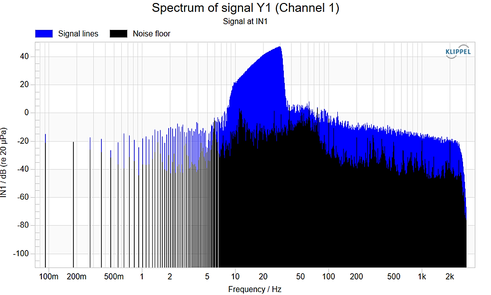
For checking the normal operation of the MPM it is recommended to view the results of the main measurement 3 TRF Measurement Sweep. Clicking on this operation will open the default windows. The window \(Y1(f)\) Spectrum shows the sound pressure spectrum measured by the microphone (blue curve) compared with the black noise floor. Sufficient signal to noise ratio SNR should be in the measured frequency range used by the sweep signal.

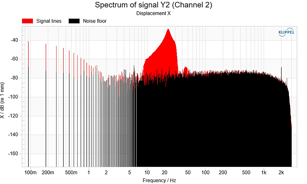
The window \(Y2(f)\) Spectrum may be used in a similar way to check the SNR of the laser displacement measurement.

The window \(Y2(t)\) shows the displacement time signal versus measurement time:

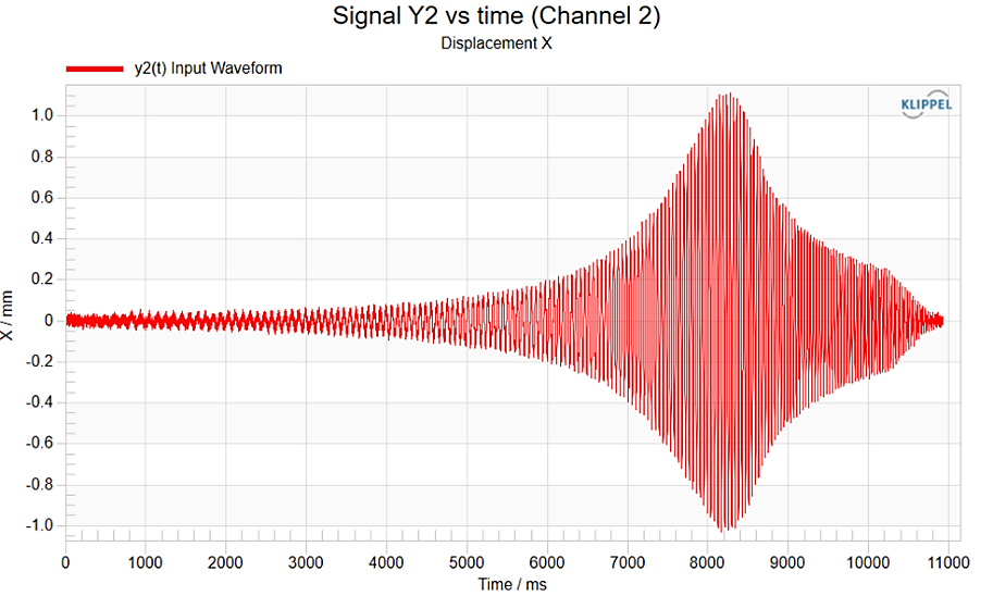
The maximal peak displacement should be at the target value defined by the user (usually 1 mm or less). Note that the displacement time function should have a symmetrical shape but not limited by the laser displacement meter.

The result of the main measurement is the transfer function shown in window \(H(f)\) Magnitude:

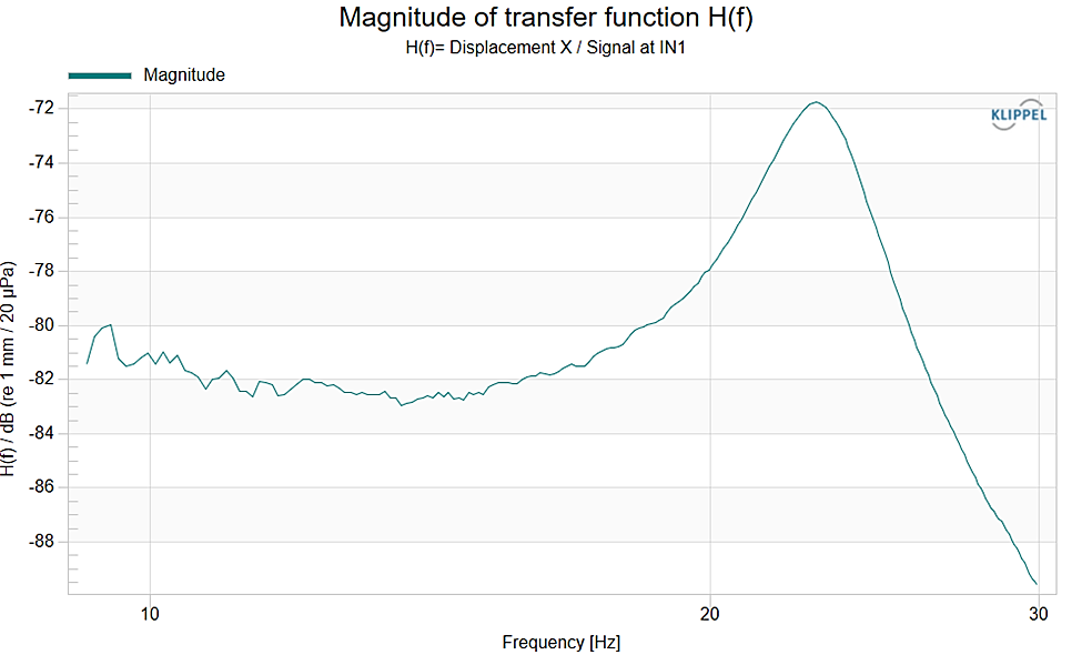
The transfer function reveals a distinct peak at the resonance frequency \(f_{\text{s}}\) which corresponds with the ratio of the Young’s modulus \(E\) (stiffness) and density (mass) of the material. For frequencies \(f < f_{\text{s}}\) the displacement is dominated by the Young’s modulus \(E\) (stiffness dominant region) while for \(f > f_{\text{s}}\) the displacement decreases by 12 dB per octave (mass dominant region). The peak at the resonance frequency compared with the displacement at lower frequencies corresponds with the \(Q\)-factor of the resonator and damping inherent in the material. If the material sample is not cut out of a plane sheet but out of a real cone additional resonance may appear in the transfer function.

Clicking on the last operation 4 CAL E Module (Results) opens the window Result Variables where the Young’s modulus \(E\) and the loss factor \(\eta\) are displayed.

Tutorial 2 – Performing a measurement

This section describes a practical measurement using the automatic software. Ensure that the hardware setup is completed and the software is installed correctly.

Selecting the Samples

This measurement technique may be applied to almost any material used in loudspeakers such as paper, rubber, plastic, fabric, metals and any compound materials.

It is recommended to use samples cut from a plain sheet, plate or foil. Samples taken from spherical cones or surround roles are problematic because the curvature in the beam makes the beam stiffer causing higher values of the measured Young’s modulus \(E\).

Paper, plastics, metals or impregnated fabric which has been bended before should not be used at all.

Many materials such as fabric are not isotropic that means the measured material properties depend on the direction of the cut.

To verify the measured parameter values it is recommended to repeat the measurement with a different batch of the material, cut the samples in different direction and clamp the sample at a different beam length.

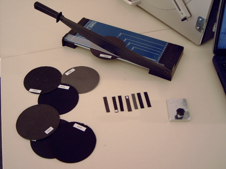
Cut the samples

The samples should be cut in small stripes 1 cm wide and 8 cm long by using a knife or a pair of scissors. It is important to have a constant width along the beam which can be ensured by using a plate shear.

Clamping the samples

Insert adjustment tool into the MPM platform.

Note

The precise adjustment of the free length of the beam is very important for an accurate measurement.

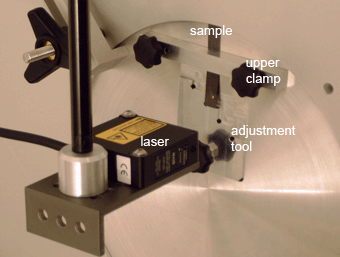
Open the two screws at the clamping beam. Small springs will move the clamping beam away from the platform. The adjustment tool provides 5 slots with different length comprising 15, 20, 30, 40, 50 mm. The sample can be inserted into the small gap and pushed down until the lower end of the sample will hit the edge of the slot. The longer the beam length is the lower the resonance frequency is. It is recommended to keep the resonance frequency between 20 and 100 Hz.

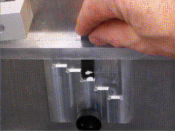
Finally, fasten both screws at the clamping beam alternatively and remove the adjustment tool.

Adjustment of the laser

The laser beam of the displacement sensor has to be adjusted to the lower end of the sample where the displacement is maximal. The vertical position can be adjusted by using the laser rod but the horizontal position (depending on the selected slot of the adjustment tool) can be adjusted by selecting the optimal hole provided on the laser ground plate.

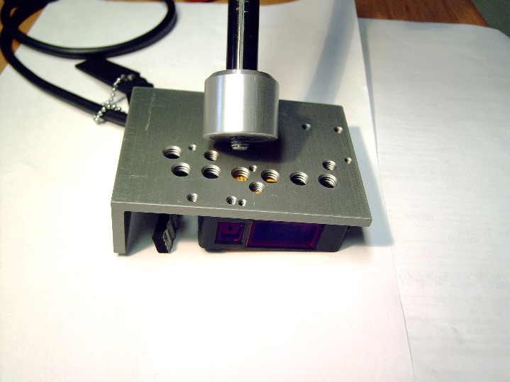
Some laser sensors require a white diffuse reflecting target surface which can be realized by making a small dot of white ink on the sample. We recommend to use laser sensors (e.g. G 32) usually intended for measurements on tweeters and telecommunication drivers because the sensitivity is high and the peak-to-peak displacement is sufficient.

Adjust the laser to the center position which allows to measure maximal positive and negative displacement of the sample.

Laser Accuracy Check

After the hardware installation it is required to check the laser calibration. The R&D System Manual describes how to

• Verify the calibration (Hardware Manual - Laser Accuracy Check)

• Calibrate the laser if calibration is not valid (Hardware Manual - Laser Calibration)

A laser with a higher resolution in a measurement range of –2 mm \(\leq x \leq\) +2 mm displacement is recommended for MPM measurements. It is suggested to use a translation stage for laser accuracy checks and laser calibration. The “spacer” used for laser accuracy checks for SPM application doesn’t match with the required range of displacement here. More information for verification and calibration of the laser can be found in the Hardware Manual.

Prepare the Measurement

After starting the application “MPM Automatic” provided in the Windows Start menu under

Start ‣ All Programs ‣ Klippel Analyzer ‣ MPM ‣ MPM Start

the following user interface will be displayed:

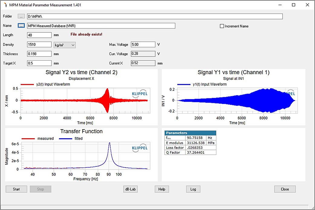
The following input information are requested:

Folder-Button “…”

Select a place where the data should be stored.

Name-Input-Field

Insert a measurement name that is used as database file name

Name-Button “…”

Open a database file to display setup and results

Length

Insert the length of the beam in mm according to the slot used in the adjustment tool

Density

Insert the density of the material sample in kg/m³ or in g/cm³

Thickness

Insert the thickness of the probe in mm

Target X

Insert the peak displacement which should be used as a target value

Max Voltage

Insert the maximal voltage used as upper limit for the voltage adjustment

Increment Name (Optional)

Every new measurement will increase the number appended to “Name”. This helps with measuring many test objects and avoids overwriting your recent data.

Run the Measurement

Press the Start button on the VB application.

Note

If no hardware is connected, a dialog will ask you to connect a device for which you have a valid license to run the operations. Additionally, the dialog allows selecting between multiple devices. You can view the devices and licenses currently installed using db‑Lab: Click the dB-Lab button and select Help ‣ About ‣ File Information.

The application performs a series of pre-measurements running in a loop to automatically adjust the stimulus (voltage and frequency range of the sweep). The instantaneous voltage and the resulting displacement will be displayed during the measurement. If the target displacement cannot be accomplished within 10 measurements a warning will be generated. If the resonance frequency is beyond the allowed limits an error message will be generated and the measurement will be aborted.

The Start button is disabled during the measurement. You may cancel the measurement at any time by pressing the Stop button.

Command Button

Comment

Start

Starts a measurement sequence of pre- and main measurements followed by calculation of results.

Stop

Stops the whole measurement immediately.

dB-Lab

Opens the operation 4 CAL E modulus (Results) in dB-Lab, where you can review setup and results in detail. See Tutorial 1.

Help

Opens the online help.

MAT Output

Opens a form for debugging purposes.

The most important results of the measurements are already displayed after successful finish of the measurement. To view detailed results, you can open the database in dB-Lab.

Results

Interpretation

upper left window

Shows the displacement versus measurement time. Note that there is a distinct peak at the resonance. An asymmetrical shape of this curve may be caused by the laser which limits the signal. Ensure that the laser is adjusted to the center position correctly and the laser is capable of handing the peak displacement.

upper right window

Shows the transfer function \(X(f)/p(f)\) versus frequency. Also in this window should be a distinct peak at the resonance frequency.

lower left window

Shows \(Y1(t)\), the sound pressure versus measurement time at input channel 1.

lower right table

Shows the resonance frequency, Young’s modulus \(E\), loss factor \(\eta\) and \(Q\)-factor in dB. If a malfunction is detected an error or warning message is displayed here.

current voltage

Voltage during the current pre-measurement

current displacement

Peak displacement during the current pre-measurement

\(f_{\text{res}}\)

Modal resonance frequency (see Physics of the MPM)

Young’s modulus \(E\)

Modulus of elasticity in tension or compression

loss factor \(\eta\)

\(\triangle f_{3 \text{dB}}/f_{\text{res}}\)

\(Q\)-factor

\(1/\eta\)

Error \(E\)-modulus

Expected Error from Air load. The Air load creates a bias, decreasing the measured \(E\)-modulus.

Error \(Q\)-Factor

Expected Error from Air losses. The Air load creates a bias, decreasing the measured \(Q\)-Factor.

Note

The graphics in the MPM application can be maximized to the full screen size by using the right mouse button. It is also possible to export and import the curves to other applications via the clipboard. However, it is recommended to view the results in dB-Lab (see Tutorial part 1). Use the button dB-Lab to start the current active database.

Tutorial 3 – Customizing MPM

The measured values of the Young’s modulus \(E\) and loss factor \(\eta\) depend on the following measurement conditions:

Dependency on Peak Displacement

The vibration of the clamped beam becomes nonlinear at higher amplitudes. There are two reasons for this. First the peak displacement is not negligible compared to the length of the beam and the geometry changes during one cycle of vibration. Second, the Young’s modulus \(E\) and loss factor \(\eta\) is based on a linear model but the real material properties behave nonlinear at higher amplitudes of stress and strain. It is recommend to operate the beam at low amplitudes (\(<\) 0.2 mm) where the nonlinearities are negligible.

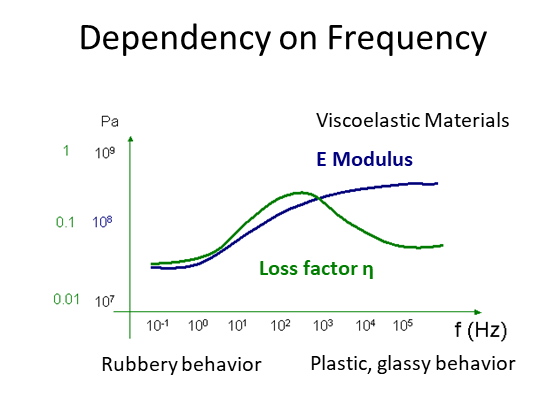
Dependency on Frequency

The measurement technique used in the MPM is based on the measurement of the first mode of the beam clamped on one side. The parameters are valid for this frequency only which should be documented in the following way:

\[E=2000\:\text{MPa}\:@\:f = 90\:\text{Hz}\]

To compare different materials it is recommended to adjust the length of the clamped sample in such a way to get a similar resonance frequency in both measurements.

Dependency on Temperature

The material parameters depending not only on the frequency, but also on the temperature.

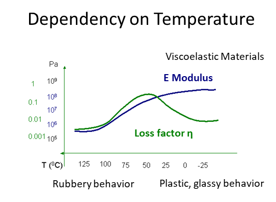
Some materials show a similarity in the dependency of Young’s modulus \(E\) and loss factor \(\eta\) versus temperature and frequency. For example, “viscoelastic materials behave colder at high frequency and warmer at low frequencies.”

Dependency on Humidity

Paper and fabric also have a high dependency on the humidity of the enclosed air. Those conditions should be controlled or at least measured and recorded together with the MPM results.

MPM - Reference

Physics of the MPM

This section gives a short overview on the physical foundations of the used measurement technique.

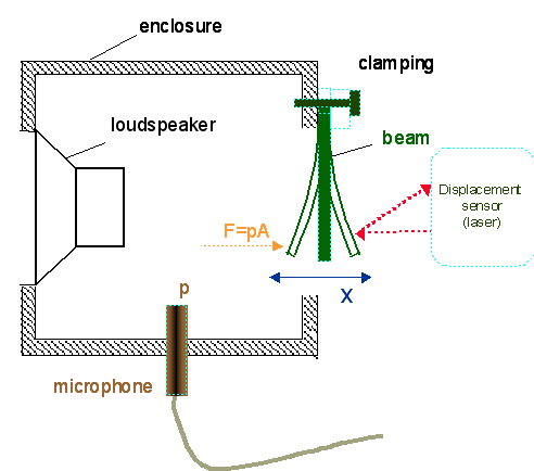
The beam is excited pneumatically by a sine sweep generated by the TRF module. During the sweep the sound pressure \(p(f)\) and excursion \(X(f)\) are measured simultaneously. \(X(f)\) is achieved from a displacement sensor (laser), which is directly mounted on the test box to minimize vibration, offset and other errors. The sound pressure is measured with a microphone which is mounted in the measurement bench. Both sensors are powered by the measurement device.

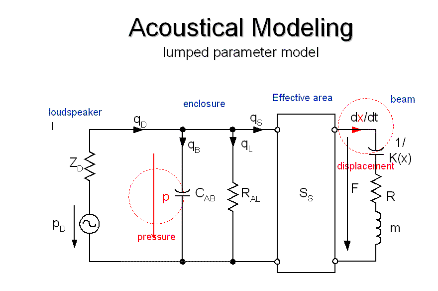
At low frequencies the setup may be modeled by the lumped parameter model shown above. The loudspeaker generates a volume velocity \(q_{\text{D}}\)

\[q_{\text{D}} = q_{\text{B}} + q_{\text{L}} + q_{\text{S}}\]

where the volume velocity \(q_{B}\) flows into the volume of the box, \(q_{L}\) is leaving the box through leaks and the volume velocity \(q_{S}\) produces the force \(F\) exciting the beam under test.

The pressure \(p\) in the box generates a force \(F = S_{\text{S}} \cdot p\) on the sample using an effective area \(S_{\text{S}}\).

The acoustical compliance \(C_{\text{AB}}\) depends on the volume \(V\) of the enclosed air and the static air pressure \(p_{0}\).

The loudspeaker used for pneumatic excitation is modeled by an acoustical impedance \(Z_{\text{D}}\) and a pressure source \(p_{\text{D}}\).

The clamped beam is described by an equivalent circuit using lumped elements. The driving force

\[F = p \cdot S_{\text{S}} = K(x) \cdot x + R(x,v) \frac{dx}{dt} + m \cdot \frac{d^{2}x}{dt^{2}}\]

is the sum of the restoring force \(K(x)\), the force \(R(x,v) \cdot \frac{dx}{dt}\) overcoming the internal losses in the material and the inertia accelerating the mass \(m\).

The measurement of the displacement \(x\) is accomplished by a laser sensor based on the triangulation principle.

The sound pressure inside the box can be measured by using a normal microphone. However, the driving force \(F = S_{\text{S}} \cdot p\) cannot be calculated in absolute values from the measured sound pressure \(p\) because the effective area \(S_{\text{S}}\) of the suspension is usually not known.

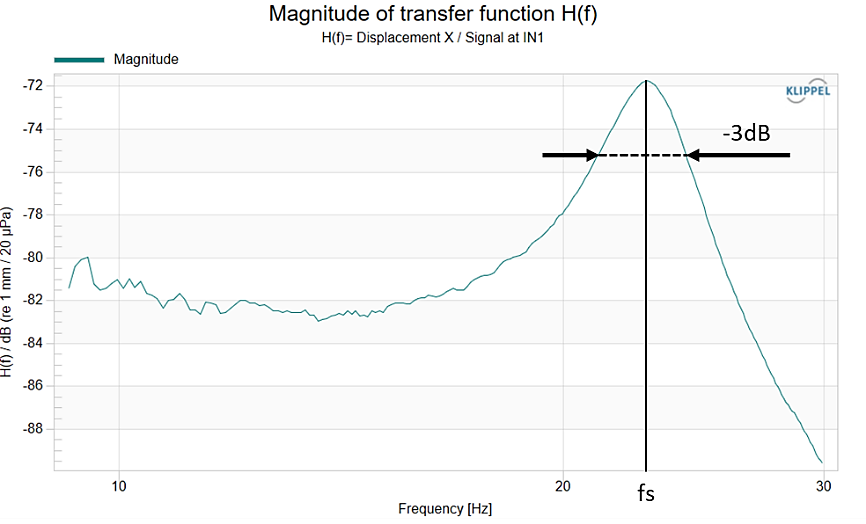
The TRF module calculates the transfer function \(H(f) = X(f) / p (f)\) which is used to determine the modal resonance frequency \(f_{\text{s}}\) and 3 dB bandwidth \(\triangle f_{3 \text{dB}}\). From these values, the geometrical parameters of the beam and its mass the modal Young’s modulus \(E\) and loss factor \(\eta\) are calculated. The calculation is done by using the CAL-module.

The different software components used in the MPM are operated by a special application software called MPM Automatic which hides the complexity of the underlying TRF and CAL module from the user and provides an easy to use interface for the necessary data input and performs all necessary measurements and calculations automatically on a mouse click.

Malfunction and Troubleshooting

Overview

This chapter will provide information that can help you solve common problems that occur with MPM measurements.

If you cannot find a description here that matches your problem, try these options:

Check the release notes Known Software and Documentation Problems that you received with your Distortion Analyzer products. This document contains the most up-to-date information about products and installation procedures.

Second, for diagnostics you can start dB-Lab using the dB-Lab Start button. When you have trouble with setup or results, then you can use the yellow envelope to include the object MPM Automatic into an email to send it to KLIPPEL support.

Error Messages

No proper amplifier output

Symptom

Error message box “No proper amplifier output. SNR lower than 35 dB.”

Remedy

• Check the power state

• Check the gain

• Check cables and connections

Low signal to noise ratio SNR in sound pressure

Symptom

The window \(Y(f)\) in 3 TRF Measurement Sweep reveals a low signal to noise ratio in the sound pressure signal.

Remedy

Check the microphone (position in the box, microphone power enabled, using input IN1 of the Measurement Hardware DA2 or KA3)

Low signal to noise ratio SNR in displacement

Symptom

The window \(Y2(f)\) in 3 TRF Measurement Sweep reveals a low signal to noise ratio in the displacement signal.

Remedy

There are two possible causes

Cause 1: Insufficient laser signal:

• Check the laser displacement sensor (optimal laser type, optimal distance to the target, sufficient reflection)

Cause 2: No sufficient movement of the beam of the material to be tested

• Use a longer beam if material is very stiff.

• Increase Max Voltage (Usually 2 V are sufficient).

Resonance frequency is too low

Symptom

The resonance frequency is too low (\(<\) 20 Hz).

Remedy

Reduce the free length of the beam using a shorter slot in the adjustment tool.

Note

If the laser beam is very short and excitation voltage high, parasitic vibration of the laser may be detected instead of the beam vibration. In this case increase the length of the beam to increase beam vibration over laser vibration.

Resonance frequency is too high

Symptom

The resonance frequency is too high (\(>\) 100 Hz).

Remedy

Decrease the free length of the beam by using a shorter slot in the adjustment tool.

Peak displacement is too low

Symptom

After 10 iteration the desired peak displacement TargetX has not been reached. CurrentX is lower than TargetX.

Remedy

• Check the laser sensor for proper operation

• Increase the free length of the beam: Recommended values: 40 mm \(\leq\) Lenght \(\leq\) 50 mm

• As last remedy, increase Max Voltage, but keep it below 2 V to avoid parasitic laser vibration

Peak displacement is too high

Symptom

After 10 iteration the desired peak displacement TargetX has not been reached. CurrentX is higher than TargetX.

Remedy

• Reduce the free length of the beam. Recommended values: 40 mm \(\leq\) Lenght \(\leq\) 50 mm

• Increase TargetX. Recommended values: 0.1 \(\leq\) TargetX \(\leq\) 0.5

Stop at maximal iteration

Symptom

After 10 iteration the desired peak displacement as defined on the input property page under target displacement has not been realized.

Remedy

Repeat the measurement. If the problem persists then contact KLIPPEL support.

The curves Y1Fund, Y1Noise, Y2Fund, Y2Noise have not the same data length.

Symptom

The curves Y1Fund, Y1Noise, Y2Fund, Y2Noise have not the same length (see input property page in step 4 CAL E module (Results)).

Remedy

Copy and paste the curves of step 3 TRF Measurement Sweep into the input property page in step 4 CAL E module (Results). See Cannot check SNR, missing curve data of for a description of the curves.

Summary file does not exist

Symptom

Unexpected error: The open command failed.

Remedy

Please contact KLIPPEL support.

Warning Messages

Cannot check SNR, missing curve data of

Symptom

One of the curves is not provided for calculation of SNR in displacement or sound pressure.

Remedy

Copy and paste the curves Y1Fund, Y1Noise, Y2Fund, Y2Noise from the original curves of step 3 TRF Measurement Sweep.

Chart \(Y1(f)\):

• Y1Fund = Curve: “Signal Lines”

• Y1Noise = Curve: “Noise floor”

Chart \(Y2(f)\):

• Y2Fund = Curve: “Signal Lines”

• Y2Noise = Curve: “Noise floor”

Cannot store xpeak into summary.txt

Symptom

There is no displacement provided in the input property page in step 4 CAL E module (Results).

Remedy

Use MPM Automatic to avoid this problem or resolve the problem by copying the curve \(y2(t)\) from 3 TRF Measurement Sweep into in_y2.

Cannot write into summary.txt. Invalid in_path

Symptom

in_path is not available on the system or is empty.

Remedy

Use MPM Automatic to avoid this problem or check the in_path parameter in the input property page in step 4 CAL E module (Results).

Low mass: Mass of moving air accounts for approximately

Symptom

Measured material is very thin and light weight, so the moving air has a significant influence on the measurement results. The Error in the moving mass is indirectly proportional to the error in the Young’s modulus \(E\) and additionally affects the \(Q\)-factor.

Note

It is not possible to compensate this error, because this error is generated based on a typical air mass which is not accurate enough for compensation.

Low losses: Losses of air accounts for approximately

Symptom

Measured material has very low losses, so the losses by the air have a significant influence on the measurement results. The error in the measured losses is proportional to the error in the \(Q\)-factor for low errors.

Note

It is not possible to compensate this error, because this error is generated based on a typical air losses which are not accurate enough for compensation.