NRL – Nonlinear Residual Analyzer

NRL - Reference

Overview

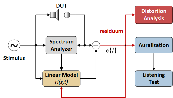
The Nonlinear Residual Analyzer is a tool dedicated to measure active or passive audio systems with music, speech or any other test signal. Based on the monitored signals, the NRL determins the linear transfer function of the device under test adaptively and separates the linear response from distortion components (e.g. non-linear or Rub&Buzz). This combination of modern measurement and listening techniques (auralization) helps to understand and evaluate the sound quality of your audio product.

Typical Setups

External Source

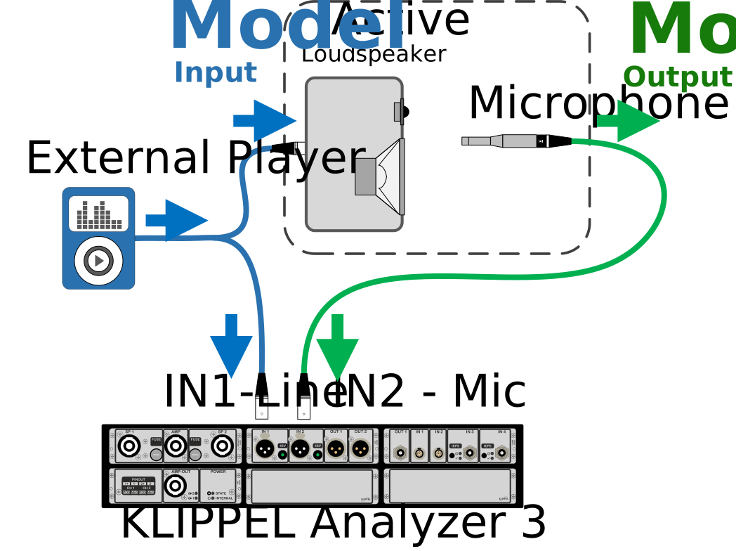
Using an external player, the NRL can be used as a monitoring tool. This measurement setup gives the highest flexibility on the stimulus. Use critical music, vary the volume live and play with filters and DSP.

Internal Stimulus

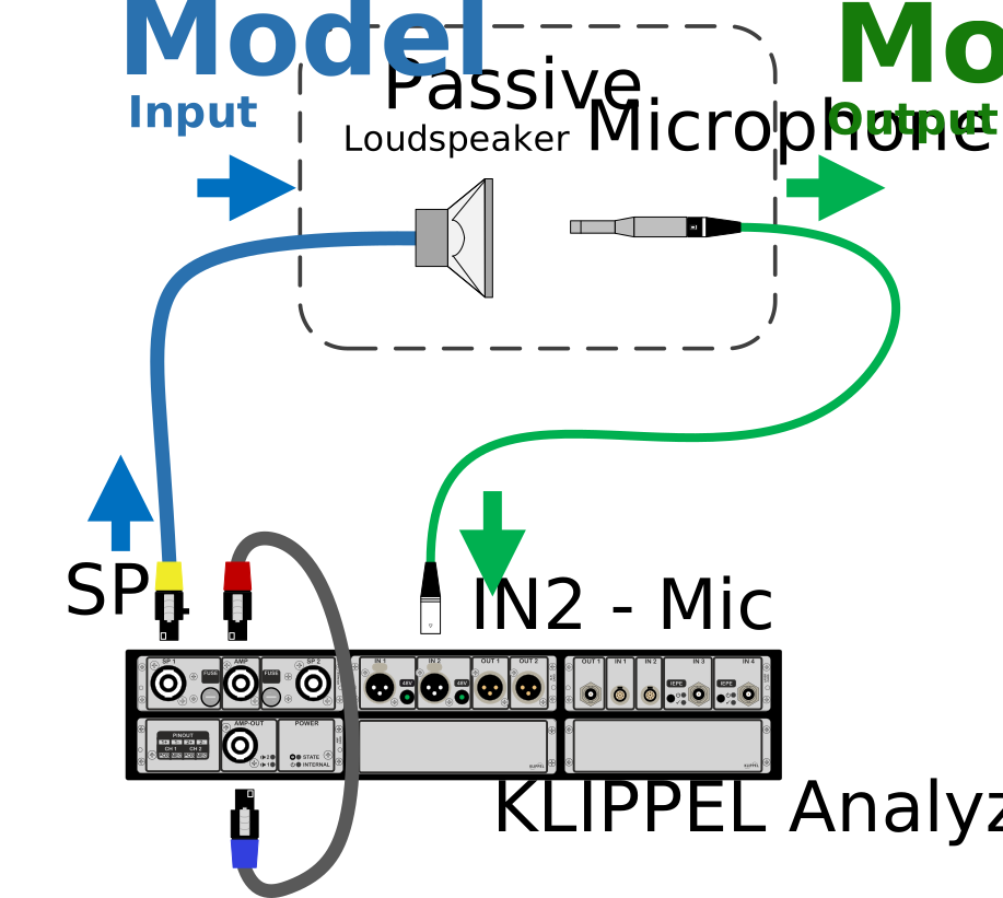
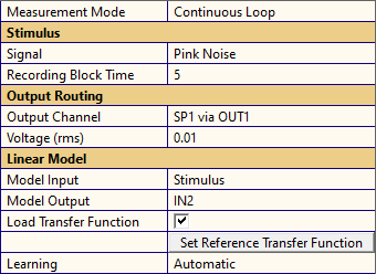
Furthermore, the signal can be played by the KLIPPEL Analyzer 3 hardware. You can use predefined stimuli like pink or white noise or any wav-file (e.g. music). In this setup, the stimulus signal is controlled by the analyzer hardware, which can provide a specified peak or RMS voltage to the device under test.

Persistent Excitation

The NRL modelling algorithm is determining the linear transfer function of the analyzed system (e.g. loudspeaker) adaptively.

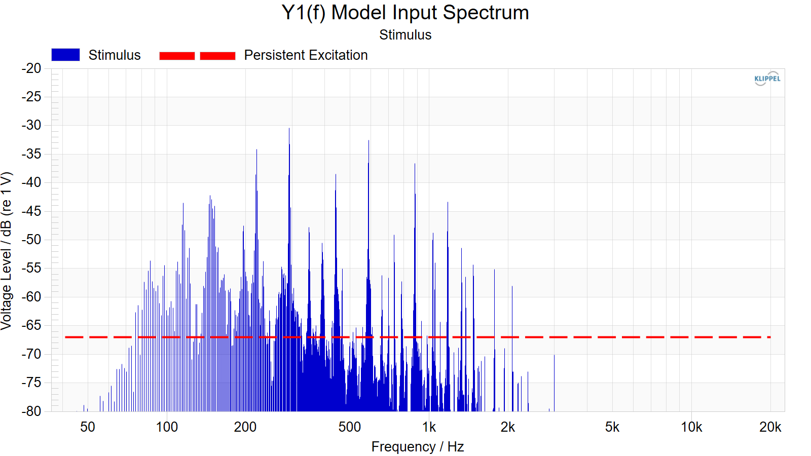
However, times of silence, when input and output is measurement noise, can cause problem for a lot of linear modelling algorithms. To overcome this problem, the NRL automatically analyzes the input level and limits the learning rate, when the input level is below the persistent excitation threshold.

pink noise	piano music

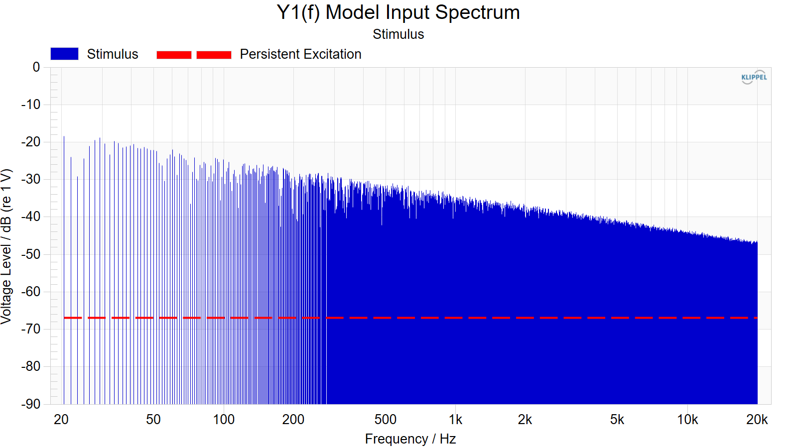
For example a broadband stimulus, like pink noise, excites all frequencies, which ideal for an initial identification and fast learning.

On the other side, piano music can have a narrow band and sparse spectrum, which could be beneficial to analyze certain loudspeaker defects and artefacts, but excites only a fraction of the passband. However, for this example the NRL limits the learning above 2 kHz automatically, which gives maximum robustness. Thus the modelled transfer function is stable and will not be corrupted.

Property Pages

Setup

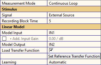
Measurement Mode

Parameter defines how the NRL is performing the measurement. The following option are available:

• Single Measurement: NRL performs a single measurement (for wav-playback the complete audio-file is played once)

• Continuous Loop: Recording is repeated automatically in an infinite loop

Stimulus

Signal

Selection of stimulus signal. The following optiosn are available:

• External Source: Signal is generated by an external player and is NRL is only monitoring the signal

• White Noise: NRL plays a white noise stimulus via the KA3

• Pink Noise: NRL plays a pink noise stimulus via the KA3

• WAV File: NRL plays a wav-file from the hard drive via the KA3

• File

  File path of the wav-file

• Select Channel

  Channel of the wav-file (e.g. left or right channel for a stereo file)

Recording Block Time

Length of a recording block in s.

Note

The NRL is performing a block wise playback and signal analysis.

Output Routing

Output Channel

Selection of the output channel for playback of the stimulus via the KA3.

Voltage (peak)

Output voltage of the stimulus.

• for white and pink noise this value defines the RMS voltage of the stimulus

• for wav-files this value defines the peak voltage of the signal

Linear Model

Model Input

Sensor signal at the input of the linear model. Typically, stimulus signal sent to the DUT.

Available signals are:

• Stimulus(f) (only for internal stimulus)

• IN1(f) Line (optional microphone calibration possible)

• IN2(f) Line (optional microphone calibration possible)

• U(f) Voltage

• I(f) Current

• X(f) Displacement

• Add. Input Gain

  Gain to amplify the input signal of the linear model to ensure persistent excitation. (for External Source only)

Model Output

Sensor signal at the output of the linear model. Typically, microphone signal measured at the output of the DUT.

Available signals are:

• Stimulus(f) (only for internal stimulus)

• IN1(f) Line (optional microphone calibration possible)

• IN2(f) Line (optional microphone calibration possible)

• U(f) Voltage

• I(f) Current

• X(f) Displacement

Load Transfer Function

Loading and storing the modelled transfer function.

On: NRL will continue the modelling with the transfer function of the previous measurement. This can be used to do an initial identification with a broadband excitation (e.g. noise), which is ideal to learn the linear system fast. As a 2^nd step, the measurement can be continued with music, which may have a sparse spectrum.

Off: NRL ignores previous runs and will start the modeling with a flat transfer function.

Set Reference Transfer Function

Button to store the current transfer function of the linear model as a reference.

This reference can be used to analyze modifications on the device under test live (e.g DSP or EQ settings) or to monitor time variant behavior of the DUT (e.g. thermal compression).

Learning

Defines the learning speed of the linear modelling.

• Learning Rate

  Definition of the custom learning rate.

Display

Frequency Range

Maximum Frequency

Maximum displayed frequency in Hz

Minimum Frequency

Minimum displayed frequency in Hz

Transfer function

Normalize to Reference

If checked the Transfer function result graph is showing a relative transfer function based on the reference. This can be used to analyze thermal compression.

Note

To use this option a reference transfer function must be set before.

Result Frequencies

Definition of the displayed frequency resolution of the transfer function. The following options are available:

• Full

• R10 (3 pts/oct)

• R20 (6 pts/oct)

• R40 (12 pts/oct)

• R80 (24 pts/oct)

• Custom

The bandwidth of the R series uses the preferred frequencies as defined in ISO 3, ISO 266 and IEC 61260.

• Frequency Resolution

  Custom frequency resolution in points per octave.

Smoothing

Parameter to smooth the transfer function with a specified bandwidth.

Spectrum

Band Integration

Parameter to display integrated spectra for a defined bandwidth. The following options are available:

• Full (no integration)

• R10 (3 pts/oct)

• R20 (6 pts/oct)

• R40 (12 pts/oct)

• R80 (24 pts/oct)

• Custom

The bandwidth of the R series uses the preferred frequencies as defined in ISO 3, ISO 266 and IEC 61260.

• Bandwidth

  Custom integration bandwidth of spectra

Weighting

Parameter to display the spectra of acoustic signals A-weighted.

Auralization

Select Signal

Selection of the signals to be auralized.

• Gain Residuum

  Gain to amplify or reduce the residual signal.

Export Folder

Folder in which the auralized wav file should be exported.

Export as wav

Button to start the export of the auralized signals

Open Export Folder

Button to open export folder in the explorer

Result Windows

Waveforms

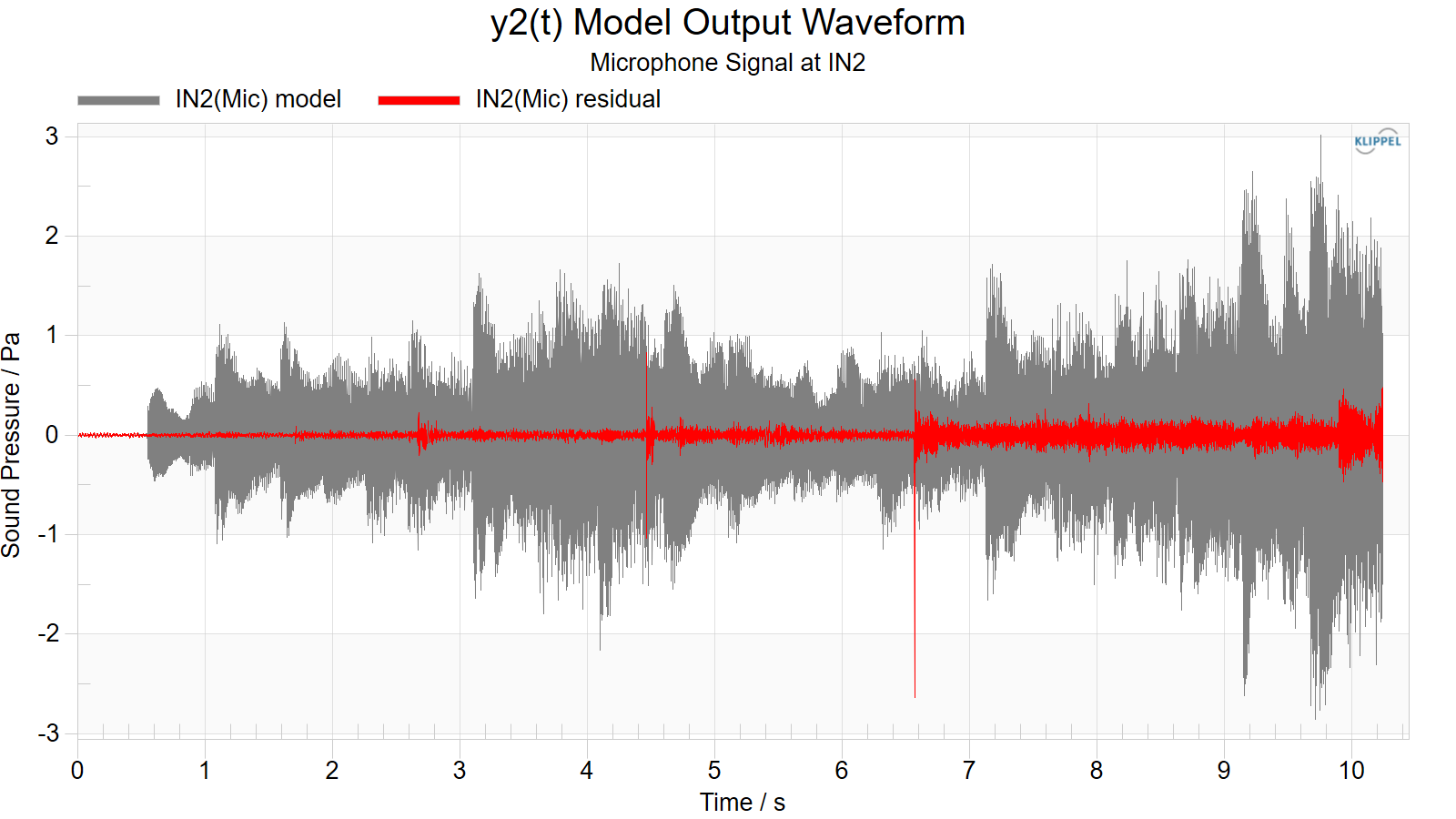
The NRL is simultaneously measuring 2 signals which are displayed in the waveform graphs.

In addition to the sensor data, the graph y2(t) Model Output Waveform includes the identified linear signal (model) as well as the isolated distortion signal (residual).

Note

For a perceptual evaluation, these signals can be exported as wav files via the Auralization tab of the Property Page.

Spectra

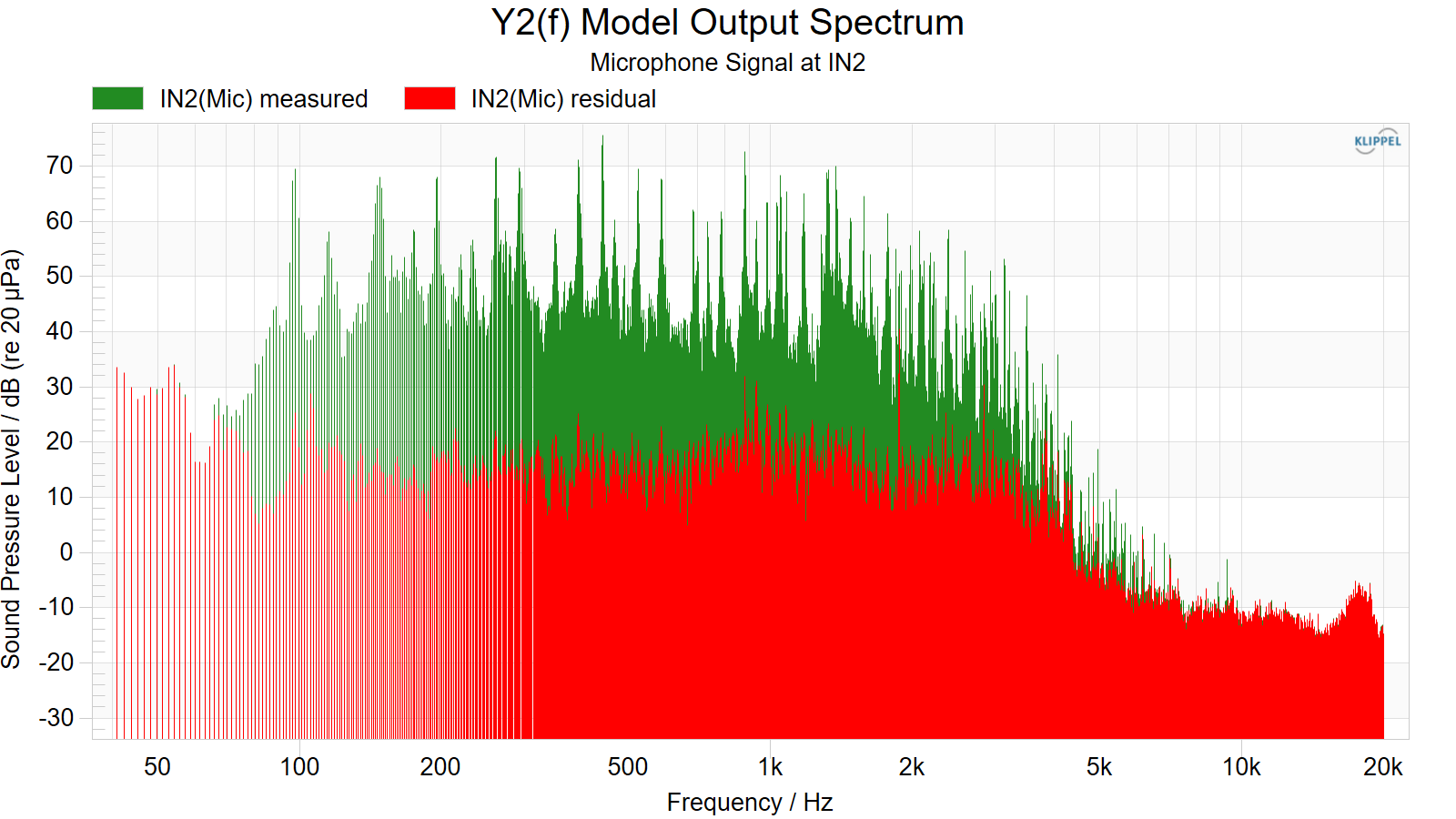
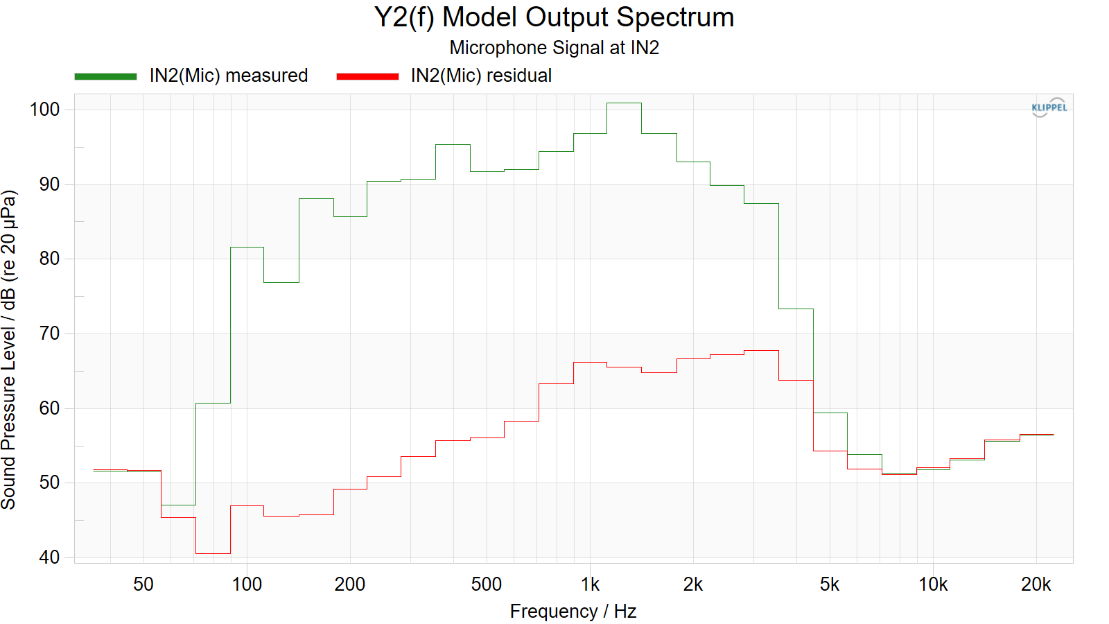
The result windows show the RMS spectra of the captured signals.

The spectra \(Y(f)\) are based on the Fourier transform of the signals (stimulus or any monitored signal).

For all monitored signals, the displayed magnitude is calculated using

\[L_{y}\left( f \right) = 20 \cdot \lg\left( \frac{\left| \underline{Y} \left( f \right) \right|}{\sqrt{2}} \right)\:\text{dB}\]

Every signal can be displayed with different resolutions e.g. Full (top) or R10 with 3^rd octave resolution) (bottom). The bandwidth can be defined in Display tab of the Property Page.

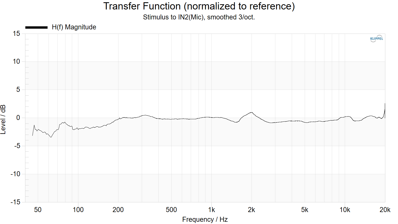
H(f) Transfer function

Shows the transfer function of the identified linear system. In order to monitor time variant behavior (e.g. compression), a reference transfer function can be set.

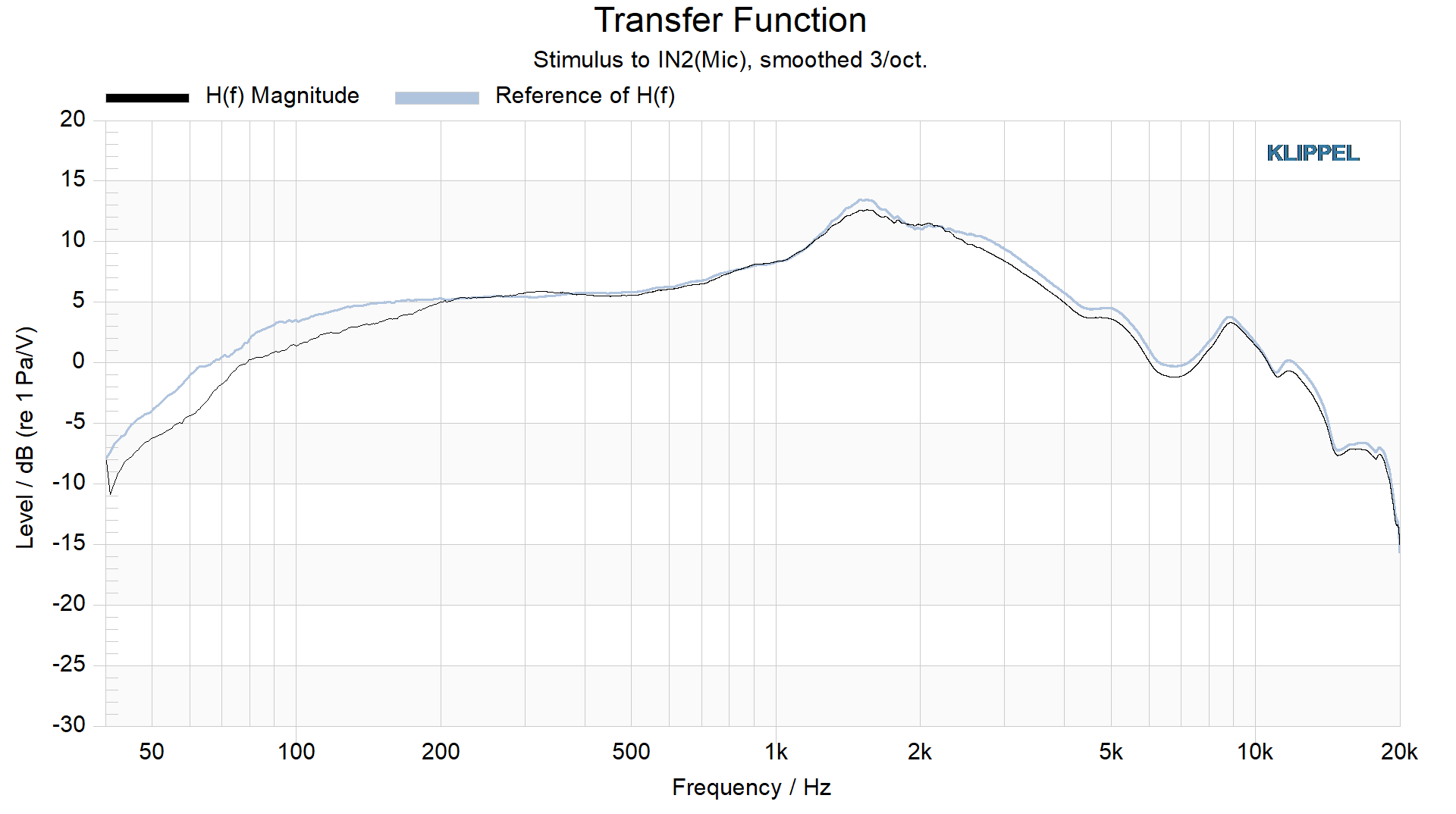
In addition, the transfer function can be normalized to the reference to analyze relative changes.

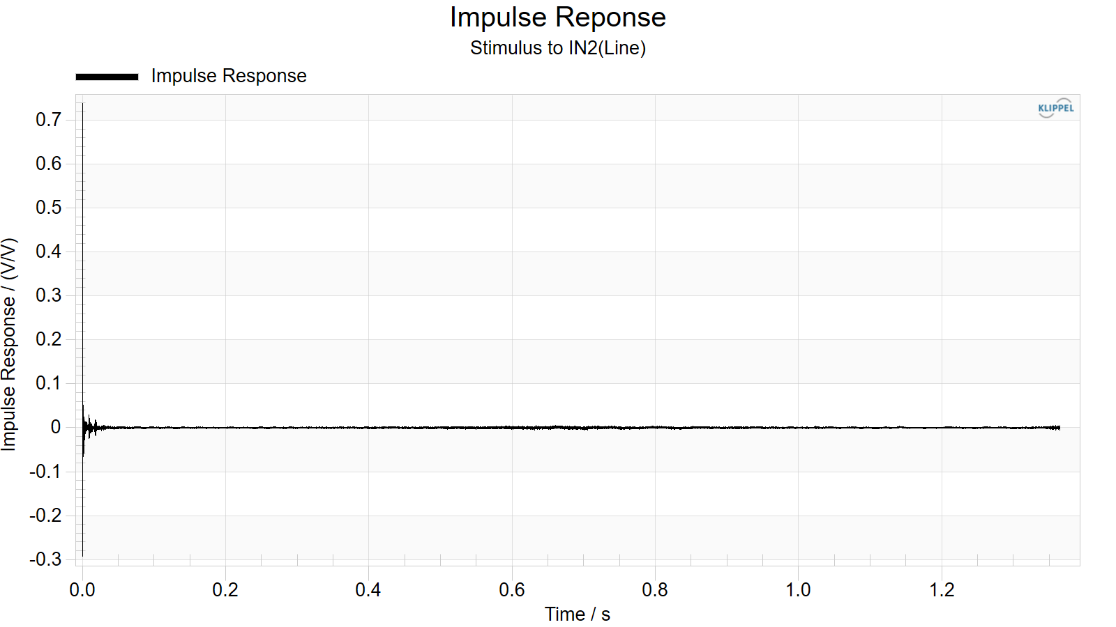
Impulse Response

The result window shows the impulse response of the identified linear model. The impulse response is calculated using the invers Fourier transformation of the captured transfer function \(H(s,t)\).

\[h\left( t \right) = \mathcal{F}^{- 1}\left\{ H\left( s \right) \right\}\]

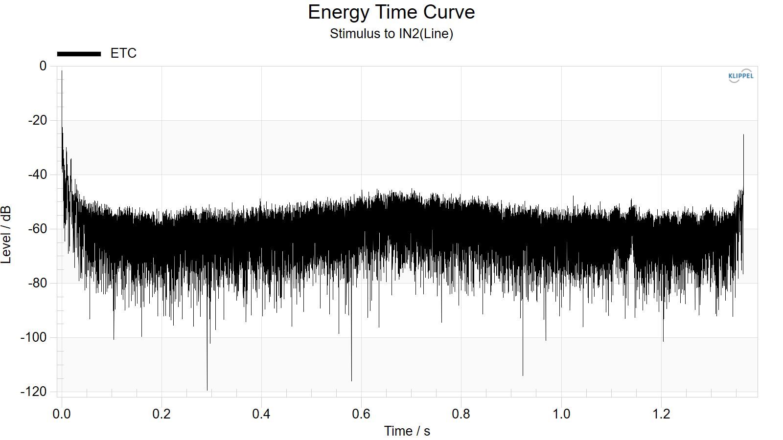
Energy-Time Curve

The energy-time curve (ETC) is the envelope of the impulse response given in dB.

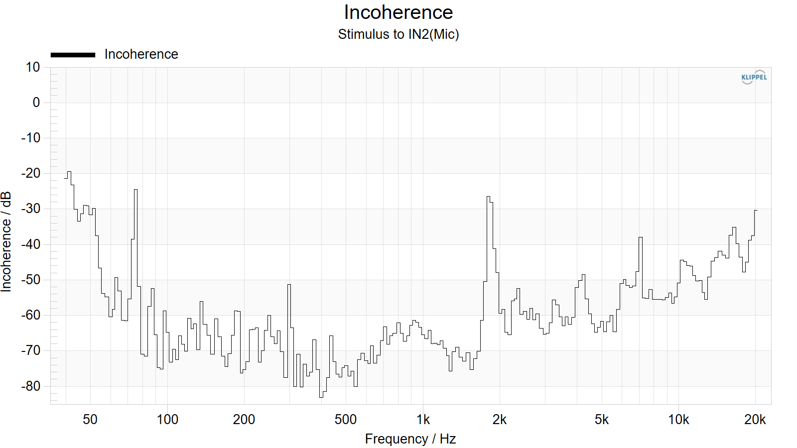
Incoherence

The coherence

\(C_{\text{xy}}(f)\ \) is a statistical parameter that examines the linear dependency between two signals \(x\) (e.g. generator output) and \(y\) (analyzer input, typically DUT output) of a system over frequency.

\[0 \leq C_{\text{xy}}(f)\ \leq 1\]

The incoherence is simply derived from the coherence by the difference to one and it can be displayed as a level in dB

\[10 \cdot \lg\left( 1 - C_{\text{xy}}(f)\ \right)\: \text{dB.}\]

For audio system testing, the incoherence is a very universal tool to evaluate non-linear signal distortion (e.g. harmonics, IMD) generated by the DUT for any broad band test signal.

Note

In addition to distortion and DUT noise, any uncorrelated signals such as sensor noise or ambient disturbance also reflect in the incoherence. Therefore, ensure that the test level is high enough, that the stimulus spectrum is dense and that only the pass-band of the DUT is tested to ensure sufficient SNR and meaningful Incoherence reading at any frequency.

Envelopes

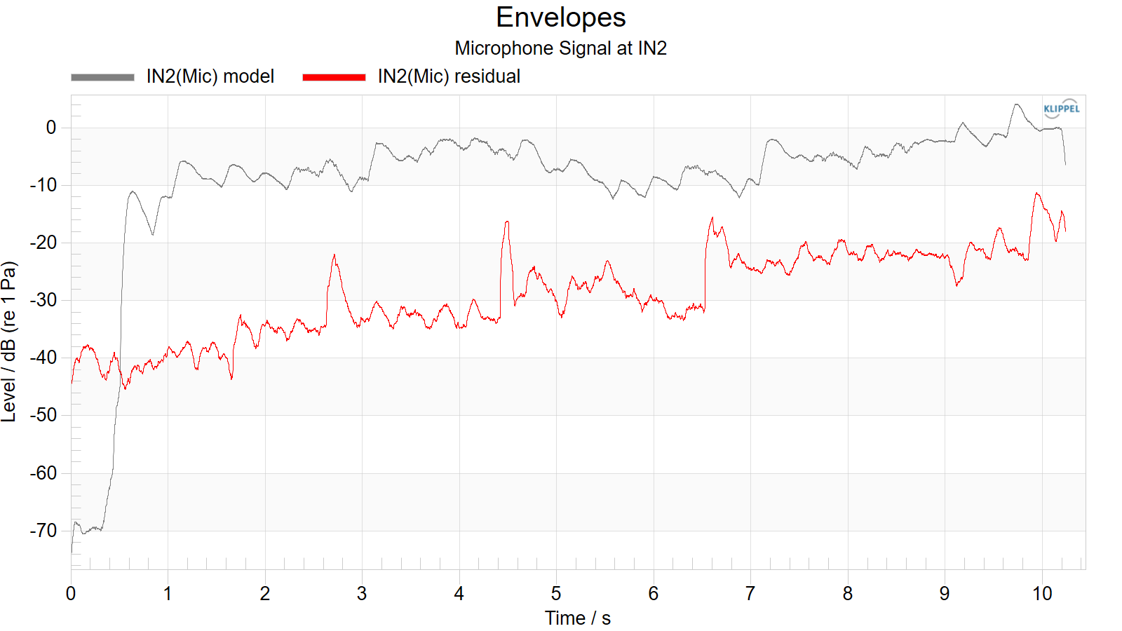
The graphs shows the envelopes of the linear and residual signal displayed in dB. These measures are the base for the distortion analysis.

Absolute Distortion

The distortion window displays absolute peak and RMS values of the linear and the distortion signal.

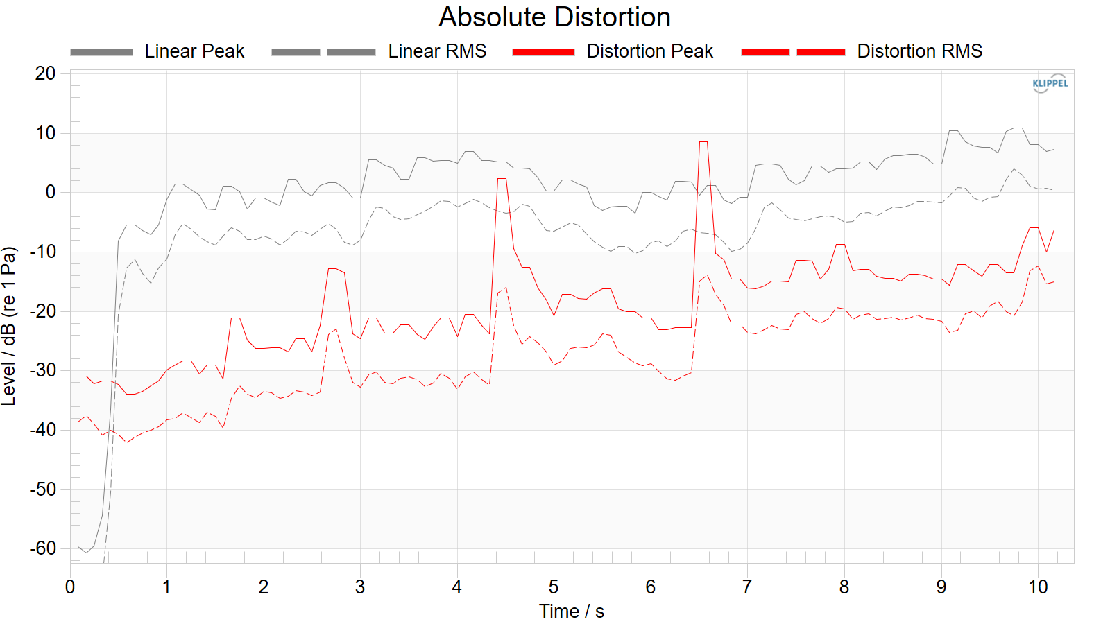
The peak distortion level helps to identify instantaneous distortions, whereas the mean level reveals dominant nonlinear distortion active over long time. The peak and RMS values are calculated based on the envelopes.

Relative Distortion

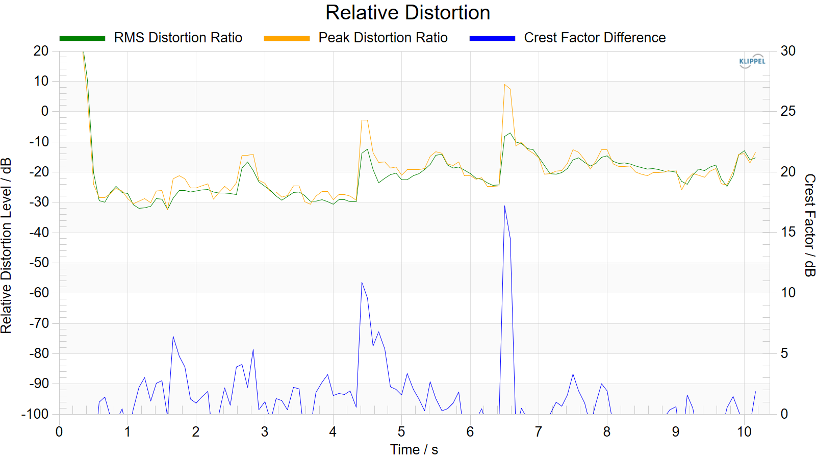
The graph shows the relation of the distortion signal versus the linear signal. If a sufficient signal to noise ratio is available (e.g. the excitation signal is significant louder than the noise floor), these values give an overview on the amount of distortion components in the measured signals.

In addition, the graph is showing the crest factor of both linear and distorted signal. In case of impulsive distortion (e.g. Rub & Buzz) the residual signal typically shows a high instantaneous crest factor. Such a click can be easily detected by the crest factor difference \(\mathrm{\Delta}C\) calculated by:

\[\mathrm{\Delta}C = C_{\text{lin}} - C_{\text{dist}}\]