
PP – Post Processing Task#
PP - Tutorial#
The Post Processing (PP) Task is an auxiliary task providing an expanding range of means or process, combine or evaluate measurement results from other tasks or external data sources.
It does not perform any measurement but may add new results (single values or curves), limit calculation options and verdicts.
Currently supported Processing options:
Two Inputs:
Difference of measured curves (e.g., Frequency Response), single values (e.g., Average Level) and absolute data (curve or single value)
Maximum Deviation of the difference curve
Mean Deviation of the difference curve
Single Input:
Calculation of maximum, minimum, mean or RMS values of user defined bands of a measured curve (e.g., Frequency Response).
Search of x-axis values where the maximum or minimum band values are located (e.g., Frequency value of Impedance peak).
More processing options will be added in future software versions. In case a particular option is important for your application, please contact KLIPPEL support and raise a feature request.
Inserting the task#
To add the Post Processing Task to your task sequence:
Select a QC test and login as Engineer
Open Property Page Tasks
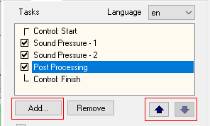
Use the Add button to include the Post Processing Task in the test sequence. It is available in the script folder Modules. The default location is:
%ProgramData%\Klippel\QC\Scripts\Klippel\QC\Modules\postprocessing.task
Make sure the new task is arranged after all tasks that provide data for processing. Use the arrow buttons to move the task within the sequence.
Note
When adding a new task, any reference data will be deleted.
Application Examples#
In this section, several examples are introduced that show the application of this task.
Stereo Headphone Application (Difference of Frequency Response Curves)#
- Setup
- Result
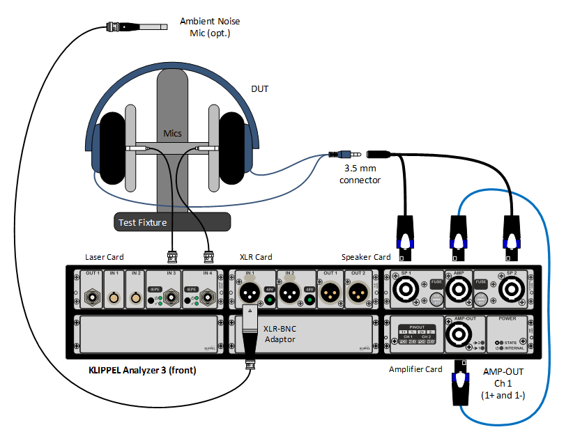
Stereo Headphone Test Setup (wired, may be also wireless, e.g. Bluetooth®)
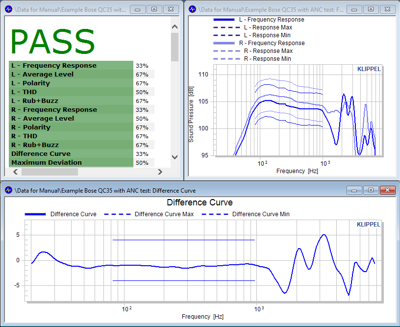
The deviation of frequency response curves between left and right ear channel may be easily calculated using the Post Processing Task. In addition, the maximum deviation at any frequency may be calculated and checked against limits.
Active Noise Control (ANC) Headphone Performance#
- Setup
- Result
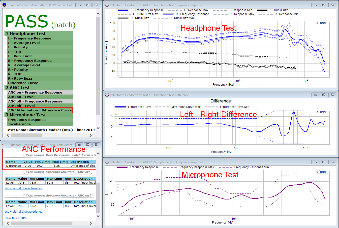
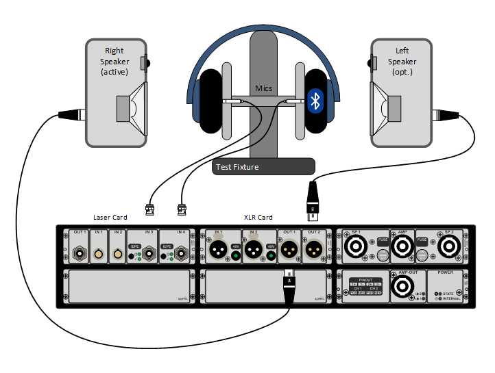
Stereo ANC Headphone Test Setup (operated wireless by Bluetooth®, may be also wired)
The performance of active noise cancellation effects can be measured by a two-step test.
In a first step the average level as a reference without ANC is measured in a defined frequency band. The typical test signal is (pink) noise, that is radiated by two or more speakers simulating a typical environment. Two microphones mounted in a test fixture record the passively attenuated noise level. For such measurements the Spectral Analysis (SAN) task can be used.
For the second step the active noise cancellation is activated and adds especially at low frequencies considerable higher noise attenuation. The achieved ANC performance is the difference between both levels from step 1 and 2 for each channel (left and right) individually.
In this example the average levels are compared, hence no curves are available but the ANC performance is available as a single value result in a table (in the example almost 10 dB in a frequency range from 80 Hz to 500 Hz). Clearly the frequency dependent performance can be tested as well using input spectrum instead of the average level.
Maximal Distortion in Multiple Bands#
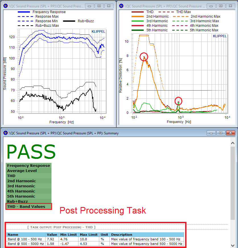
The maximal distortion value may be easily calculated in multiple bands using the Post Processing task . The calculation can be applied to any distortion curve (THD, 2:sup:`nd` Harmonic…) at the frequency bands defined in the parameter page.
In the following example, the max. THD is calculated in 2 different bands:
Low frequency band: from 100 to 500 Hz
High frequency band: from 500 Hz to 5 kHz
Minimal Impedance of a Bass Reflex System#
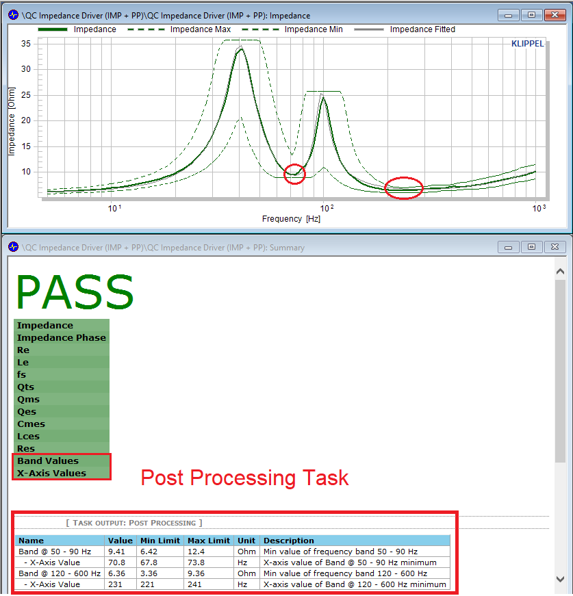
The minimal impedance value as well as its frequency may be easily calculated using the Post Processing Task. In the following example, the impedance curve of a vented box system is measured. An approximation to the vented box resonance and its impedance (minimal value between the both peaks), as well as the minimal impedance from transducer resonance frequency are calculated and checked against limits.
Note
For a better calculation of the vented box resonance frequency, please refer to the Impedance task, which offers an accurate Thiele/Small parameter fitting including the vented box resonance frequency obtained in this example.
PP – Reference#
In this chapter all parameters of the Property Page Tasks are described.
Section Configuration#
- Processing
Main parameter to configure the whole post processing task according the number of inputs:
Two Inputs
Single Input
The following data formats are supported:
Frequency Response
Impedance
Other Curve
Measured Value
Absolute
Use and combination of the input data depends on the processing and results. Details for each type are given below.
Note
In case of different frequency axis of input data, the axis of data#2 is interpolated to the frequencies found in data#1. The difference is calculated in the overlapping range of the frequency axis only.
- Frequency Response / Impedance
These input data are predefined curves as they are the most often curve types for difference option. Thus, only the task which measured the curves, need to be defined.
- Other Curve
Any other curve which is provided by measurement tasks can be used for post processing. Measure and task name must be defined. If no measure or task with the defined name can be found, a list with all available curves and tasks are listed in the error message:
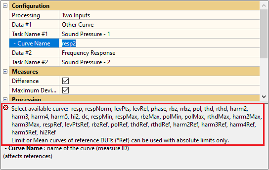
Note that limits (
*Max,*Min) and reference DUTs mean curves (*Ref) are available after calculating limits only. Thus, they are not available yet for the actual limit calculation process. This is the reason, why those curves can be processed with absolute curves only.Note
The labels for results are not identical with the displayed labels. Internal names are used to specify the data in a unique way.
- Measured Value
Any measured single value (e.g. average level from SPL task) can be used for post processing. Values can be combined with curves. The frequency axis of the curve is used for the result.
If two values are processed, the result is shown in chart Summary. No curve is available.
- Absolute
Any curve can be specified. If two inputs are processed, the frequency axes must overlap. A value shall be specified as a single number.
Note
For dynamic values or curves from external sources, the External Devices (EXD) task may be used to read value from devices or files. They are then available as Curves (see Other Curve) and can be used for processing.
Section Results#
Processing Option Two Inputs#
Two results are available and can be activated:
Difference Curve#
In most cases the result of the difference option will be of curve type and is displayed in Chart Difference. If the result is a single value, the difference will be displayed in a table in Chart Summary.
Limits can be applied.
Maximum Deviation#
The maximum deviation provides the simple max value of the difference. It can be used to assess the absolute peak value of the difference result curve. It is available for curve type only. The Difference Measure must be activated to use the Maximum Deviation Measure.
Limits can be applied.
Mean Deviation#
The mean deviation provides the mean or RMS value of the difference curve. It is available for curve type only. The Difference Measure must be activated to use the Mean Deviation Measure.
Limits can be applied.
Processing Option Single Input#
Two results are available and can be activated:
- Band Values
Calculates the maximum, minimum, mean or RMS values of the user defined bands in processing parameter Band Definition. Results and limits are displayed in a table in Chart Summary.
- X-Axis Values
Searches the x-axis values where the maximum or minimum values calculated in Band Values modes max or min are located. X values and limits of each band will be added to the results table in Chart Summary.
Section Processing#
Processing Option Two Inputs#
- Max, Mean Deviation – F min
Lower frequency limit for Maximum and Mean Deviation results.
- Max, Mean Deviation – F max
Upper frequency limit for Maximum and Mean Deviation results.
- Mean Deviation - Mode
Mean Deviation calculation mode:
Mean
RMS
- Mean Deviation – Data Type
Data type of difference curve required in Mean Deviation result:
Linear
Level (dB): data is interpreted as logarithmic level (dB) data. Mean value is calculated after converting the curve into linear data (antilog). Afterwards, the result is converted again into a logarithmic value (dB).
Processing Option Single Input#
- Band Definition
Definition of bands used in Band Values result. A numeric identifier ID can be set optionally.
Format 1 (without ID):
[freq1-min freq1-max
 freq2-min freq2-max
 ...       ...      ]
Format 2 (with ID):
[band1-ID freq1-min freq1-max
 band2-ID freq2-min freq2-max
 ...      ...       ...      ]
- Band Values - Mode
Band Values calculation mode:
Max
Min
Mean
RMS
- Band Values – Data Type
Data type of input curve required in Mean and RMS calculation modes:
Linear
Level (dB): input data is interpreted as logarithmic level (dB) data. Band values are calculated after converting the input data into linear data (antilog). Afterwards, the results are converted again into logarithmic values (dB).
- Band Values – Unit Y Axis
Unit of Band Values is required if input data Data #1 is Other Curve. This unit is displayed in results table in Summary window and is used in post processing tools as Yield Statistics (YST) and Statistics (STAT).
- Band Values – Unit X Axis
X-Axis unit of Band Values is required if input data Data #1 is Other Curve and result – X-Axis Values is activated. This unit is displayed in results table in Summary window and is used in post processing tools as Yield Statistics (YST) and Statistics (STAT).
Section Display#
Processing Option Two Inputs#
- Diff – Ymax / Ymin
For the chart Difference, the Y-axis may be restricted to a user specified range in order to ensure a constant part of the curve and ease the optical appearance of the difference curve for operators.
- Custom Color of Difference Curve
A user defined color may be specified in case multiple Post Processing Tasks are within a test sequence.
Limits#
Activate the Limit Mode on Property Page Limits to access the limit parameters. Limit parameters are available for the activated results only. See the QC User Manual for details in chapter Test Configuration / Limit Calculation.
Processing Option Two Inputs#
- Difference Curve
Available limit calculation modes are:
Shifting Limits
Statistics (Standard Deviation), also combined with Shifting Limits
Absolute (Absolute Limits), also combined with Shifting Limits
Alignment of Limits to level or best fit
Jitter
- Maximum Deviation
Available limit calculation modes are:
Shifting Limits
Statistics (Standard Deviation)
Absolute (Absolute Limits)
- Mean Deviation
Available limit calculation modes are:
Shifting Limits
Statistics (Standard Deviation)
Absolute (Absolute Limits)
Processing Option Single Input#
- Band Values and X-Axis Values
Available limit calculation modes are:
Shifting Limits
Statistics (Standard Deviation)
Absolute (Absolute Limits)
Supported formats of Shift and Sigma (Statistics) Masks, as well as Absolute Min and Max Parameters:
If ID is not available in Processing parameter Band Definition:
Single row: limit applied to all bands.
Same number of rows as Band Definition: each limit row is applied to its corresponding row of Band Definition.
In addition to previous formats and if band ID is available in Processing parameter Band Definition:
One row including ID for each band limit to be applied. In next example, no limit is defined for the 2nd band (band2-ID), which results in a VOID verdict for this band:
Band Definition:
[band1-ID freq1-min freq1-max
 band2-ID freq2-min freq2-max
 band3-ID freq3-min freq3-max]
Shift Mask:
[band1-ID band1+shift band1-shift
 band3-ID band3+shift band3-shift]
