DIS – Distortion

DIS – Distortion#

Overview#

This measurement module performs a comprehensive distortion analysis. It measures the fundamental, harmonic, intermodulation and DC component versus voltage and frequency of the excitation signal.

Based on the Analyzer hardware unit two signals may be recorded in parallel and analyzed in the post processing. Voltage and current at speaker terminals as well as displacement and any external sensor signal may be used for Distortion (DIS) measurements.

During the measurement driver protection is provided. The measurement is interrupted if the increase of voice coil temperature and/or the total harmonic distortion in the measured signals exceeds specified limits.

DIS Tutorial#

This tutorial makes you familiar with the DIS module.

The tutorial is divided into three parts.

In the first Viewing DIS Results we will show you how to view DIS results already stored in the web example database. Short background information on distortion generation is given.
The next part of the tutorial Performing a new DIS provides a save step-by-step recipe to measure harmonic distortion in sound pressure and displacement.
In the final section Customizing DIS we discuss modifications of the setup parameters to use more powerful features and to improve the performance of the measurement. Intermodulation measurements are described and hints for excitation setups depending on the measurement target are given.

In the chapter DIS Reference you will find a detailed description of the result windows and the configuration of the property pages.

Viewing DIS Results (Part 1)#

Example data used in this manual is stored in the Web Example database. If not downloaded already, get it from the latest R&D release and open the web-based database.

Measurement Results#

The example measurement analyzes harmonic distortion excited by a sweep over 20 to 200 Hz in frequency and over a level range of 1 to 4 V. Since distortion are effects of the nonlinear behavior of loudspeakers they always should be measured for multiple frequencies and multiple levels. The DIS module allows specifying both sweeps within one measurement.

The default result windows show the total harmonic distortion, 2^nd and 3^rd order harmonic distortion and the fundamental component of the excitation tone. All components are measured with a microphone and shown in dB / SPL.

Note

Please note, that all changes of measurement setup data will clear the example measurement data since result and setup information must be kept absolute synchronously. This is not valid for display setup data. It is recommended to work with a copy of the example database.

Step by step instructions are given to get a first impression of the variety of DIS results.

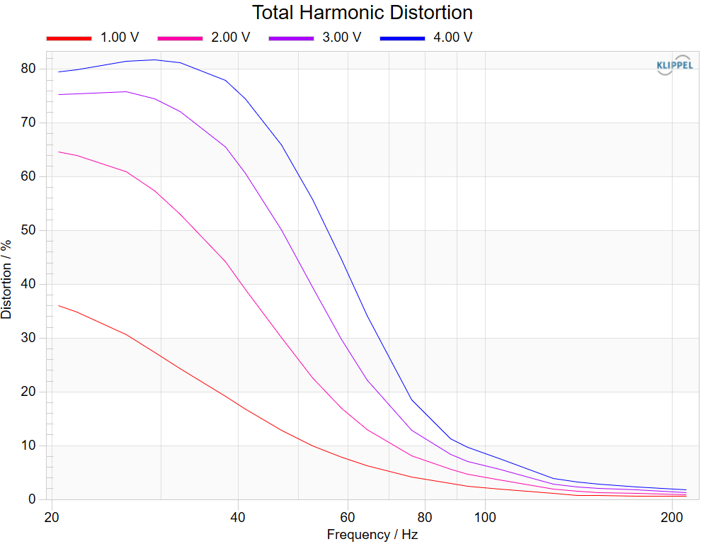
For very low frequencies the Total Harmonic Distortion is above 80 %. This is due to a very high excitation level and mechanical limiting of the suspension system. The dominant contribution comes from 3rd order harmonic. The cause for these high values is the nonlinear stiffness. The symmetrical shape produces 3^rd order distortion at low frequencies. The 2nd order harmonic component is also relatively high and is produced by the asymmetrical shape of thestiffness characteristic of this driver (may be investigated from the LSI operation results of the same Example Speaker 2).
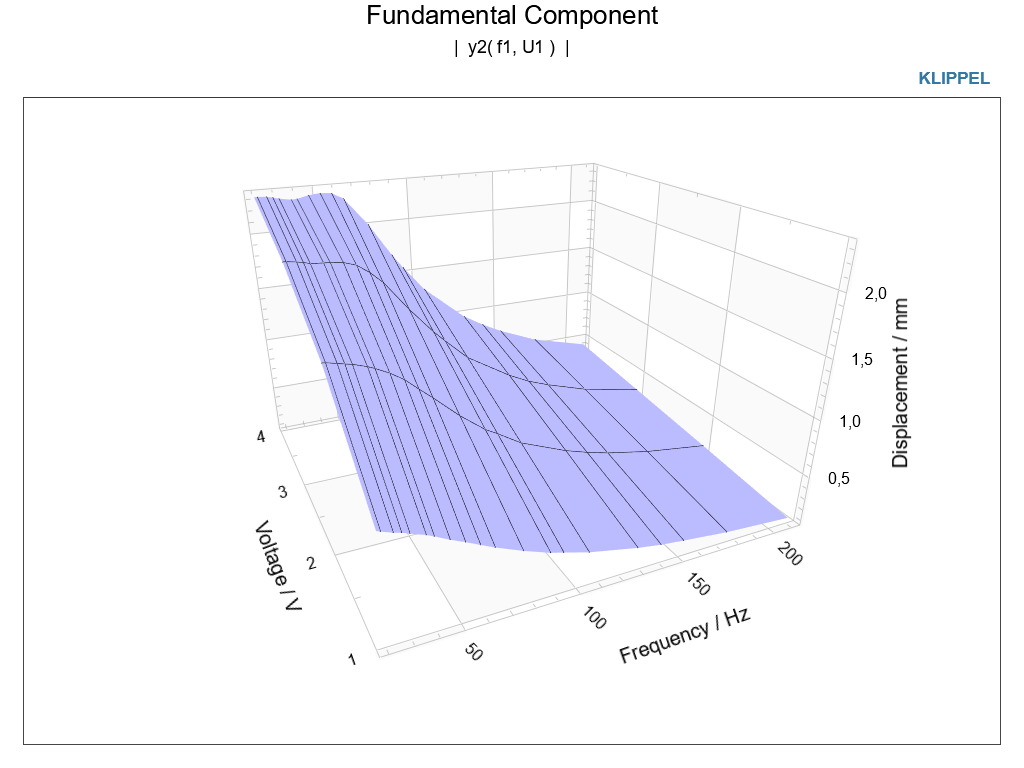
Go to the property Page DISPLAY and modify the Plot Style to 3D plot. Change also the State signal to Displacement X.

Confirm with Enter. Looking at the fundamental component the 3‑dimensional graph of frequency and voltage sweep response is shown. At high voltages and low frequencies, the mechanical compression is clearly visible. The excursion can’t rise proportional with excitation voltage since the suspension limits. However, the basic property of displacement dependent on frequency is also visible. From DC to resonance frequency the amplitude of excursion is almost constant and falls down with 12 dB/octave above resonance frequency.

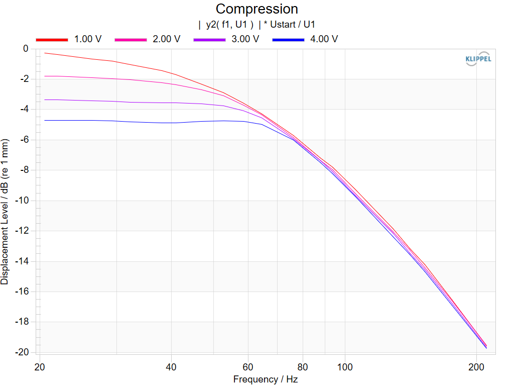
Switch Plot Style back to 2D and open the window Compression from the result windows list. The above discussed mechanical compression of the fundamental component is clearly visible. Here the fundamental component is linearly downscaled according to the voltage levels. In other words, the increase of voltage is compensated. For a linear system all curves must lay over each other since the output signal of a linear system rises with the same gain as the input signal does. For 4 V excitation at low frequencies, the fundamental component is compressed by almost 5 dB.
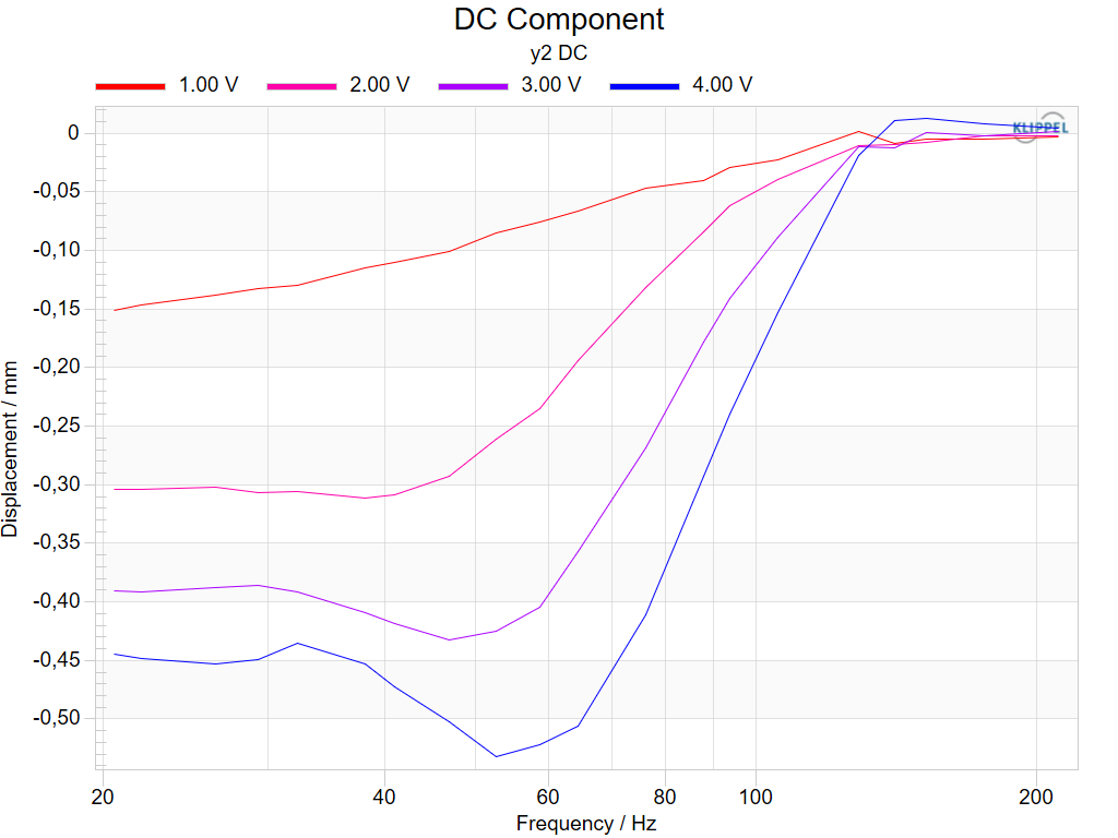
Open the result window DC Component from the result windows list. Here the dynamically generated DC component of the driver is shown. Dependent on frequency and level the AC part of the excursion due to the (pure) AC excitation is superimposed by a DC part. This DC part is generated by the nonlinear characteristics of the driver. In this example the stiffness is not symmetrical. This shifts the momentary rest position to negative displacements (towards the magnet structure of the driver, moves in).
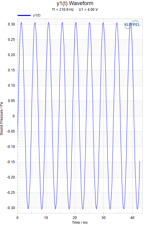
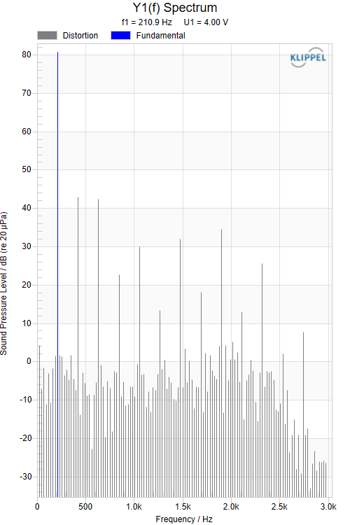
Open the result windows Y1(f) Input Spectrum and y1(t) Input Waveform and look at the spectral components and the time signal of the sound pressure signal. In order not to inflate the database size the spectra and waveforms are stored only for the last sweep point (rather than for all sweep points). The spectrum and time signal you look at is therefore the data for the last sweep point measured. Since the displacement and therefore the harmonic distortion is low for higher frequencies, the time signal looks very sinusoidal. However, in the spectra clearly the harmonic components are visible.

Note

The magnitudes given in all spectral representations are RMS magnitudes. (i.e. \(\text{peak magnitude} / \sqrt{2}\)). For consistency reasons displacements are given in mm (RMS). The corresponding peak displacement is calculated by multiplying the given displacement by \(\sqrt{2}\) . An exception is the DC component where the RMS value is equal to peak.

Especially for comparing the DC component with the fundamental (which is given in RMS) care must be taken to consider an additional factor of \(\sqrt{2}\) .

Performing a new DIS (part 2)#

This part of the tutorial will guide you to perform a new measurement using the DIS module. At the beginning a short overview over the setups is given. With a step by step guide a first measurement of the harmonic distortion of SPL in the near field as well as in the displacement will be performed and the results will be analyzed.

Requirements#

For performing the guided measurement, you need the following requirements:

Klippel Analyzer unit, Power Amplifier, Cable
Microphone (for Distortion Analyzer version 1.x also microphone power supply) with known sensitivity, cable from microphone to Klippel Analyzer unit input (XLR/BNC) for SPL measurements
USB capable PC, Software: dB-Lab, DIS module.
Test Loudspeaker (woofer) with \(f_{\text{s}}\) about 50 – 150 Hz mounted rigidly in Laser Stand

Connect Hardware#

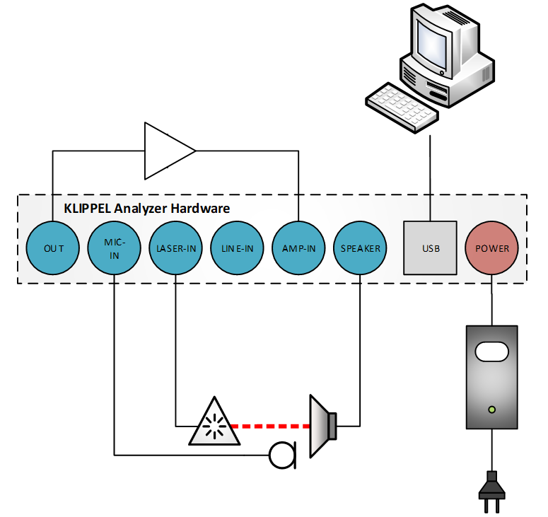
Connect the Hardware as described in the Hardware Manual (Chapter 1.2 for KA3 and chapter 1.3 for DA1/DA2). Depending on the method you use, you have to connect laser or microphone.

Note

Make a dot with white ink (correction fluid) on the diaphragm and adjust the laser to this point. Alternatively, you can use white adhesive tape that can be removed easily after the measurement. See also section 2.2 Laser Displacement Sensors in chapter Hardware of the manual for more information.

Creating a New Operation#

If you don’t have measured anything with the analyzer, please refer to the dB-Lab manual for creating a new operation, using measurement templates and navigating within databases.

It is good practice to perform all own measurements in a separate database, not to use the example database. If necessary, create a new database and insert a new, empty object (using the empty object template). Give this object an appropriate name, e.g. DIS first measurements. Then insert a new DIS operation using the operation template DIS 3D Harmonics. You may also rename the operation name. Press OK to confirm the selection.

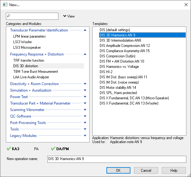
Here you can also see all other prepared templates for DIS operations (more templates may be added in a further update, please check). In the bottom line a reference to the application as well to an application note is given. In our example AN 9 deals with Harmonic Distortion Measurement. We recommend doing the guided measurement given in this tutorial first to get a basic understanding and later to work on the Application Note 9.

Setup Data#

First open the property pages to look at the setup for Harmonic Distortion measurement.

Measurement Setup#

Property Page INFO:

Here a short description is given to specify the measurement. This information may be used for report generation and templates for other measurements with similar setups..

Property Page DRIVER:

The geometry and rated values of the driver should be specified here. This page is valid for all operations of the same object, these are object specific properties. All other pages are operation related and valid only for the actual measurement operation.

Property Page STIMULUS:

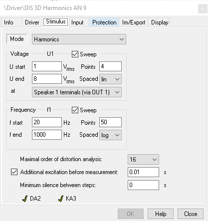
The Property Page STIMULUS specifies the frequency and voltage sweep as well as the mode of distortion measurement. Here Harmonics has been selected. Because Speaker 1 terminals were selected, the voltages specified are the voltages applied to speaker terminals (amplifier output voltages). Before the measurement an automatic amplifier check determines the amplifier gain and sets the output levels accordingly.

Warning

You must set the excitation level accordingly to your speaker under test. The given maximum voltage may damage your driver. Please start with lower voltages and increase step by step the voltage level, until considerable distortion are measurable.

Property Page INPUT:

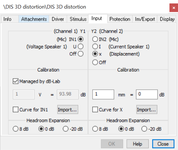
On the Input property page, the hardware routing for two parallel input channels has to be selected. For Harmonic Distortion Measurements the SPL is the most important and therefore selected. A microphone has to be connected to input channel 1 (IN1).

Note

Please note that hardware versions 1.x of the Distortion Analyzer require an additional microphone power supply.

Property Page PROTECTION:

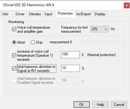
The PROTECTION page allows defining several protection limits in order to ensure safe operation of the driver. Since the DIS module measures Large Signal properties of the driver the protection should be always enabled.

Note

Temperature and distortion components rise not linear but with at least second order of the excitation voltage. Using no protection, the driver may easily be destroyed. It is the responsibility of the user to set adequate limits.

Property Page IM/EXPORT:

The IM/EXPORT page allows copying setup data to the clipboard (export) as well as importing setups from different measurements (others DIS and SIM operations). You may also check the data with the built-in clipboard viewer.

Property Page INPUT:

In the INPUT page the sensitivity of the connected sensors must be specified. As the Laser sensor is factory calibrated, the microphone must be software calibrated by the user. If you have calibrated a microphone and stored the sensor calibration file, you can simply select the file in the sensor menu and leave the checkbox Managed by dB‑Lab checked. If you want to override the calibration for this operation, uncheck the checkbox and enter the microphone sensitivity in the group Calibration (on the left-hand side for input IN1 and on the right-hand side for input IN2). Enter for instance 0.034 V = 94 dB for a sensitivity of 34 mV/Pa.

Display Setup#

Property Page DISPLAY:

The DISPLAY property pages do not affect the measurement but only the representation of the results. You may change all settings also after performed measurements. 3D- or two 2D- graphical representations and the signal to be analyzed (one of the two chosen in the INPUT Property Page) may be selected.

To modify scaling, colors or labels please double click on the graph and change the settings.

There is also a context sensitive menu (right mouse button) for each graphical window available to copy and paste curves, enable cross cursor functionality, marking measured points as well as exporting graphs and data to several formats. For more details, please refer to the dB-Lab manual.

Start Measurement#

Please make sure before measuring that the hardware is connected correctly and that the excitation voltage is specified at the driver terminals and not too high for your driver (property page STIMULUS).

Start measurement by pressing Run .
After some (silent) initial tests (where the amplifier gain, the amplifier distortion and the DC voice coil resistance are measured) you will hear the measurement sweeping through the specified frequency-voltage points. At the very bottom of the dB-Lab window the measurement progress will be shown.
In case of any problems, you may pause the measurement by pressing Pause .

The measurement will be canceled if you press Cancel .

Wait until the measurement has finished.
The measurement will automatically finish and return to the standby mode (icon visible). Please wait until all result windows has been updated.

Viewing and checking results#

Please open the default windows of the operation by double click on the operation name in the object tree window.

Select the Fundamental + Harmonics graph from the result window list (click on the checkbox left from the result name). Check first the fundamental, if there is a correct SPL frequency response signal shown. If not, please refer to the Malfunction and Troubleshooting at the end of the DIS-manual.

Note

Please note that in these windows only the last (and highest) voltage level over frequency is shown.

Check also the 2^nd and 3^rd harmonic distortion. If possible, please compare the results with your traditionally used measurement system. Please ensure identical excitation levels and conditions (microphone position) etc. Make sure that the sensitivity of your microphone is correctly specified in the INPUT property page.
A good test for a valid measurement is to check the time and frequency characteristics. Please open the result windows y1(t) Input Waveform and Y1(f) Input Spectrum. They show the waveforms and spectra for the last sweep point. In order to keep the size of the database reasonably small the waveform and spectra for the other sweep points are not stored.

Check the noise of the microphone signal. The fundamental and the first harmonics should be at least 40 dB above the noise level. You may compare your spectra with the spectra shown in the Tutorial part 1 in case of uncertainties. The time signal should be not distorted by noise. However, if measuring high nonlinear distortion, the time signal may not be sinusoidal anymore.
Open the property page DISPLAY. Make sure that the State Signal is set to Signal at IN1 in order to show the sound pressure signal. The default setup shows the data in 3D. However, for the beginning it might be better to visualize it in 2D versus Frequency.
While the Fundamental + Harmonics was given for the highest excitation level only, the Fundamental is given for all excitation levels. Open the result window Fundamental. If you have driven the loudspeaker into nonlinear range, you should see the compression effect due to displacement limiting. At very low frequencies increasing the input voltage will not result in proportional increase of output SPL. Since a logarithmic sweep (in voltage) is used, the same factor between successive voltage levels is set. You may also open the result window Compression to see the normalized drop in SPL of higher excitation levels.
Open the result windows 2nd Harmonic Distortion and 3rd Harmonic Distortion. Here you have the distortion components given in percent of the fundamental.

Note

Please note that at higher frequencies the properties of the environment have a strong influence on the results. External noise, reflections as well as cone modes may distort your measurements.

Please read in addition to this first guided measurement the tutorial section 3. There a lot of hints and application specific information is given. We recommend to perform several measurements with customized setups and working on the DIS related application notes.

Note

The stimulus signal of the DIS module is kept synchronous to the FFT size. This implies that only frequencies can be used that are multiples of \(\triangle f = f_{\text{sample}} / N\), where \(N\) is the signal length in samples. The program automatically maps all frequencies specified by the user to the closest multiple of \(\triangle f\). See section Difference between specified and applied frequency in chapter Malfunction and troubleshooting for further information.

Customizing DIS (part 3)#

In this part of the tutorial, we discuss modifications of the setup parameters to use more powerful features and to improve the performance of the measurement.

How to Protect Drivers#

There are two basic protection features in the DIS module (property page PROTECTION). The first one is the temperature monitoring. Between test tones a short measurement at fixed frequency and level is performed to sample voltage and current to analyze the increase of \(R_{\text{e}}\) and therefore the temperature increase (with known voice coil material specified in property page DRIVER). There is no interaction of the temperature and the distortion measurement. Having the voltage information at the speaker terminals (independent on the input signal setting) this allows checking the amplifier gain. A warning will be generated, if the amplifier gain varies during the test considerably.

Note

Please note that the temperature is sampled in between the measurement sweep points. That means that it only recognizes exceeding of the temperature limit after the sweep tone, which heats the driver. Careful setups must be chosen by the user (no too large steps in the voltage sweep) to prevent destruction.

The second protection is limiting the maximal harmonic distortion for each input signal. This measure may protect the driver mechanically. For very low frequencies where the suspension limits the drivers output high harmonic distortion are generated and may be detected e.g. in SPL or displacement.

How to Protect Drivers Connected to a Crossover#

The test measurement for temperature monitoring can be performed with different test frequencies. The frequencies may be selected by Frequency for Test in property page PROTECTION. Select a test frequency that is in the pass band for the particular driver that you want to protect. The frequency may be located near or at the roll off region of the crossover filter. However, ensure sufficient excitation for the measurement. Do not attenuate the voltage more than 6 dB.

Speed up Measurement#

There are several ways to speed up the measurement:

The measurement can be speeded up considerably if Monitoring is switched off in property page PROTECTION. In this case the voice coil temperature is not measured and no thermal protection is provided. Furthermore, it is not checked if the amplifier gain is constant during the measurement.
If you want to measure only harmonic distortion and no intermodulation distortion use the Harmonics Mode in property page STIMULUS. A simultaneous measurement of harmonic and intermodulation distortion will take considerably more time than a sole harmonic measurement.
If you intend to measure only one signal switch off the other channel in property page INPUT.

How to calibrate sensors?#

Pleas refer to Hardware manual section Sensor Handling.

How to Load a Microphone Correction Curve?#

The normalized microphones frequency response, as it is typically provided by the microphone manufacturer or calibration laboratory, could be used as a microphone correction curve. The measured input spectrum will be divided by the microphone correction curve to compensate for its frequency response. Thus, the correction curve is subtracted from the measured response curve in dB.

The correction curve may be specified

as magnitude curve versus frequency in dB or
as magnitude (in dB) and phase (in degree) curve versus frequency.
it must be normalized at the frequency the sensitivity was specified (typically 250 or 1000 Hz).

Open the property page INPUT. Select (Mic) IN1 if you want to connect the microphone to input IN1 (alternatively select (Mic) IN2 if the microphone is connected to IN2).
Press the Import… button in the corresponding group Calibration. This will open a dialog where you can import the microphone correction curve. Press the Load… button and load the file with the correction curve (see description of the required format below).

The required format for the correction curve is quite simple. It is the same format generally used within the KLIPPEL R&D System for importing or exporting curves from or to the clipboard. Each curve is represented by two columns of ASCII numbers. The columns are separated by blanks. Rows are separated by line breaks. The first column contains the \(x\)-values (frequency), the second column contains the \(y\)-values (correction in dB); see example below. Each row represents a base point of the curve. The fractional part of the \(x\)- and \(y\)-values must be separated by a dot, comma is not allowed. Any external text editor can be used to type in the two columns. If you select them with the mouse and press Ctrl + C they are copied to the clipboard. Alternatively use the clipboard editor provided by dB-Lab. It is activated by choosing View | Clipboard in the menu. Between the base points the curve is interpolated linearly. Outside the base point range, the value of the first and the last base point is used respectively (extrapolated).

Example#

The curve consists of the following the five points:

(20 Hz, -0.3 dB), (1 kHz, 0 dB), (2 kHz, 0.1 dB), (5 kHz, 0.3 dB), (10 kHz, 0dB)

The corresponding clipboard format is:

How to Load Correction Curves for Other Input Signals?#

Correction curves for the voltage, current or displacement signal are loaded in the same way like microphone correction curves (see above). Instead of selecting the microphone signal select Us, Is or x in step 1.

How to Cope With Time Delay?#

To ensure steady-state measurement conditions a pre-excitation duration can be specified in property page STIMULUS. The pre-excitation is activated by selecting Additional Excitation Before Measurement. To cope with time delay, use a pre-excitation of 0.1 seconds (corresponding to up to about 30 m microphone distance).

How to Cope With Creep?#

The creep effect can cause a considerable time constant in the displacement. In some cases, it will take up to 1 second and more until the displacement signal reaches steady-state. To ensure steady-state measurement conditions set Additional Excitation Before Measurement in property page STIMULUS to about 1 sec. You may also check the steady state condition by performing several measurements with different pre-excitation constants. Check for deviations in the DC component of the Displacement.

How to View Waveforms and Spectra?#

In order not to inflate database size the complete waveform and the according spectra are not stored in the database. However, inspecting the waveform or the spectra for specific measurement points is often quite useful. During the measurement waveform and spectra can be viewed for the most recent sweep point.

If you pause the measurement by pressing Pause , the waveform and spectra are shown in the result windows y(t) Input Waveform, Y1(f) Input Spectrum for channel 1 and y2(t) Input Waveform, Y2(f) Input Spectrum for channel 2.

After the measurement has finished the above result windows will show the waveform and spectra of the last sweep point. If you want to view the waveform and spectra for a particular sweep point, you can repeat the measurement for this single sweep point.

Press Run .

A message box will pop up where you select Single Point Measurement and the voltage and the frequency of the sweep point you are interested in. After the measurement has finished waveform and spectra are shown for the selected sweep point. The results (distortion components and distortion measures) obtained during the complete sweep will be updated with the results of single point measurement. This provides furthermore a convenient way to correct stray results.

Note

Re-measuring points will not be accurate if due to high excitation levels the temperature of the driver was considerably higher than for the new single point measurement. In this case you have to run the complete sweep and to pause for the point of interest.

How to Copy Stimulus Settings From or To SIM#

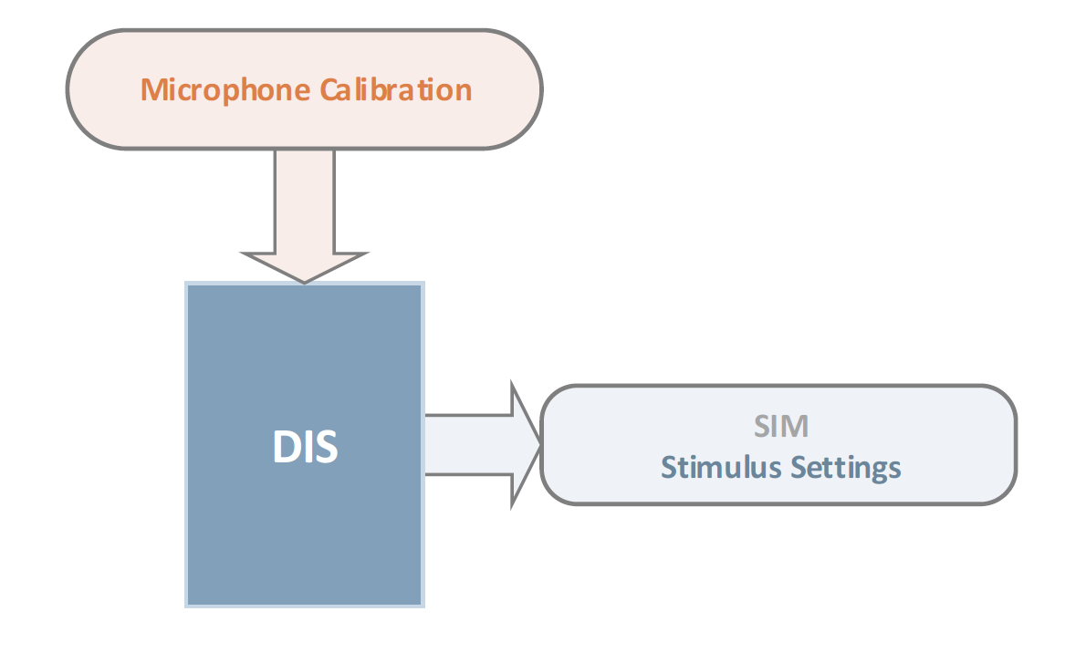
The DIS and the SIM modules may be considered as twins. Many result windows and setup parameters correspond to each other. A common application is to simulate a speaker and to compare the simulation results to the results measured with DIS. For this the same voltage-frequency sweep must be used. The Stimulus settings of SIM can easily be copied to DIS:

Open property page IM/EXPORT of a SIM operation and press Export to Clipboard .
Open property page IM/EXPORT of a DIS operation and press Import from Clipboard .

To copy the settings from DIS to SIM press first the Export button in DIS and then the Import button in SIM.

Nominal Versus Measured Voltage#

In the property page STIMULUS the nominal voltage sweep is specified. Although the amplifier gain is measured there are always small deviations from the specified voltage level.

Note

Please note, that in all result windows the specified voltage is used, not the actual measured one. In normal applications this will not result in larger errors.

However, if the voltage gain of the amplifier deviates from that measured one at the specified frequency (the pilot tone frequency of the temperature detection is used) considerable errors may occur. This may happen e.g. at very low frequencies (power amplifier high pass) or at very high frequencies (power amplifier low pass). Please make sure that your power amplifier has a sufficient bandwidth for your DIS measurements.

How to Switch 2D / 3D#

Open the Property Page DISPLAY and select either 3D or 2D versus frequency or versus voltage. Almost all graphs are controlled by this switch. However, the result window Fundamental + Harmonics is always a 2D plot.

Linear / dB y‑axis of Result Windows#

The user can adjust the spacing of the \(y\)-axis for the result windows

Fundamental
Harmonic Distortion
Difference Intermodulation
Summed Intermodulation and
Peak + Bottom

in property page DISPLAY. First, a linear (Lin) or a logarithmic (Log) spacing can be chosen. If Auto is selected the representation of the \(y\)-axis values depends on the spacing of the voltage sweep selected in property page STIMULUS (Voltage U1: Spaced). For a linear voltage sweep the \(y\)-axis values will be spaced linearly whereas for a logarithmic voltage sweep the \(y\)-axis values will be given in dB. This way amplitude compression effects can be visualized if 2D and versus f1 is selected in property page DISPLAY. In case of no amplitude compression the curves for different sweep voltages are equidistant. Any compression will alter the distance between the curves. The \(y\)-axis spacing (Lin/Log/Auto) can be selected independently for Y1 and Y2.

Note

Results will always be plotted in dB if Signal at IN1 or Signal at IN2 is selected in property page DISPLAY as these signals are normally microphone signals.

Add Comments#

The INFO property page allows the user to change the name of the measurement and to add a comment to the measurement. Comments may be included in the report file and are used for operation and object templates in all derived measurements.

DIS Reference#

Measurement Technique#

DIS module supports one or two sine tone excitation signals only. Both, amplitude and frequency may be stepped in a user defined range.

Signal Generation#

A two-tone signal defined by

\[U\left( t \right) = U_{\text{1}}\sin\left( 2\pi f_{\text{1}} \cdot t \right) + U_{\text{2}}\sin\left( 2\pi f_{\text{2}} \cdot t \right)\]

is an optimal excitation signal to measure harmonic, difference-tone and summed-tone intermodulation components. The frequencies \(f_{\text{1}}\) and \(f_{\text{2}}\) and the voltage \(U_{\text{1}}\) and \(U_{\text{2}}\) may be specified by the user. They may be varied automatically to perform frequency and voltage sweeps.

Excitation#

Frequency Sweep#

The user can choose between a single point measurement performed with constant and a series of sequential measurements performed for different values of \(f_{\text{1}}\). The user has to specify the start value \(f_{\text{start}}\) and the end value \(f_{\text{end}}\) for the frequency \(f_{\text{1}}\) as well as the number of intermediate points spaced linearly or logarithmically.

Voltage Sweep#

The user can choose between a single point measurement performed with constant and a series of sequential measurements performed for different values of \(U_{\text{1}}\). The user has to specify the start value \(U_{\text{start}}\) and the end value \(U_{\text{end}}\) for the Voltage \(U_{\text{1}}\) as well as the number of intermediate points spaced linearly or logarithmically. The voltage \(U_{\text{2}}\) of the second tone is coupled to the voltage \(U_{\text{1}}\) of the first tone and the user specifies the ratio \(U_2 / U_1\).

Measurement Modes#

Measurement of Harmonics#

The user can choose between the different measurement modes. The Harmonics mode is used to measure the harmonic components of tone \(f_{\text{1}}\). The second excitation tone is switched off. This reduces the amplitude of the excitation signal \(U(t)\) and avoids interference between harmonic and intermodulation components.

Measurement of Intermodulations#

In the Harmonics + Intermodulation (f1) and Harmonics + Intermodulation (f2) modes summed-tone and difference-tone intermodulation components (centered around \(f_{\text{1}}\) and \(f_{\text{2}}\) respectively) are measured additionally to the harmonic components of \(f_{\text{1}}\). No harmonic components are measured if the mode Intermodulations (f1) is selected. There are three different modes to specify the frequency \(f_{\text{2}}\) of the second tone:

The frequency \(f_{\text{2}}\) is held constant during frequency sweep of \(f_{\text{1}}\). This mode allows to generate very critical stimuli for most transducers. Selecting \(f_2 < f_1\), \(f_{\text{2}}\) may represent a bass tone producing large voice coil displacement and \(f_{\text{1}}\) represents any audio component (voice) in the pass band of the transducer.
The distance \(f_2 - f_1\) between both excitation frequencies is constant during the frequency sweep of \(f_{\text{1}}\). This mode produces difference intermodulation at the same frequency independent of \(f_{\text{1}}\).
The frequency ratio \(f_2 / f_1\) is held constant between both excitation tones. Selecting \(f_2 > f_1\) and using a fractional ratio (e.g. 5.5) this mode avoids interference between the harmonic and intermodulation distortion components.

Measurement of Total Harmonics + Noise#

The THDN mode is for measuring the harmonics and the total harmonics + noise. The measurement is excited by tone \(f_{\text{1}}\). The second excitation tone is switched off. The sample frequency is held constant for all sweep points to get comparable measurement conditions.

Post Processing#

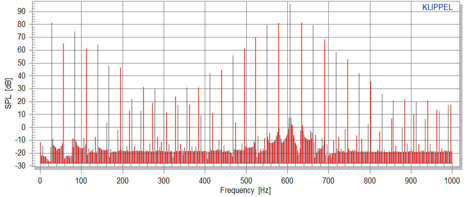
The driver variables in steady state condition are subject to a FFT analysis. Using frequencies \(f_{\text{1}}\) and \(f_{\text{2}}\) of the excitation tones at values consistent with the FFT length, additional windowing of the time signal can be omitted. This reveals the spectral components without any smearing effects.

Property Pages#

After activating DIS you can open the property pages. These pages present the setup parameters for measurement and result analysis.

INFO Page#

The INFO page allows the user to change the name of the measurement and to add a comment to the measurement (comments may be included in the report file).

DRIVER Page#

The DRIVER page contains special transducer parameters that have to be provided by the user.

Surface area: \(S_{\text{d}}\)

Effective projected surface area of the driver diaphragm
Diameter: \(d_{\text{d}}\)

Diameter of round effective radiation surface
Impedance: \(Z_{\text{n}}\)

Nominal impedance of the driver
Input Power: \(P_{\text{e}}(\text{max})\)

Maximum nominal input power
Material of voice coil: The kind of material (copper, aluminum) used for the voice coil has to be specified if known.

This information is used to identify the increase of voice coil temperature from the variations of the voice coil resistance.

STIMULUS Page#

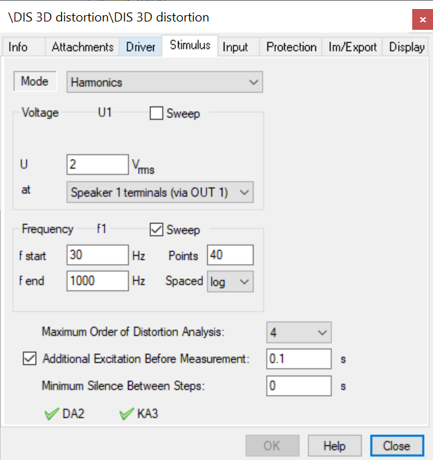
The STIMULUS page gives access to the parameters used for controlling the voltage and the frequency of the excitation signal. An “array” of voltage-frequency points can be specified. The DIS will sweep through this array and measure the distortion for each voltage-frequency point.

Mode#

There are five different measurement modes. (\(n\) denotes the maximal order of distortion analysis)

Harmonics:

Harmonic distortion are measured only. Maximum sweep frequency \(f_{\text{end}}\) is \(80\: \text{kHz} / n\)

(Distortion Analyzer 2: \(40\: \text{kHz} / n\)).

Harmonics + Intermodulations (f1):

Harmonic and intermodulation distortion centered around the excitation frequency \(f_{\text{1}}\) are measured. Maximum sweep frequency \(f_{\text{end}}\) is the minimum of \(80\: \text{kHz} / n\) and \(80\: \text{kHz} - (n-1) \cdot f_2\)

(Distortion Analyzer 2: \(40\: \text{kHz} / n\) and \(40\: \text{kHz} - (n-1)\cdot f_2\).

Harmonics + Intermodulations (f2):

Harmonic and intermodulation distortion centered around the excitation frequency \(f_{\text{2}}\) are measured. Maximum sweep frequency \(f_{\text{end}}\) is the minimum of \(80\: \text{kHz} / n\) and \(80\: \text{kHz} - (n-1) \cdot f_2\)

(Distortion Analyzer 2: \(40\: \text{kHz} / n\) and \(40\: \text{kHz} - (n-1)\cdot f_2\).

Intermodulations (f1):

intermodulation distortion centered around the excitation frequency \(f_{\text{1}}\) are measured. Maximum sweep frequency \(f_{\text{end}}\) is the minimum of \(80\: \text{kHz} / n\) and \(80\: \text{kHz} - (n-1) \cdot f_2\)

(Distortion Analyzer 2: \(40\: \text{kHz} / n\) and \(40\: \text{kHz} - (n-1)\cdot f_2\).

THDN:

Harmonic distortion and total harmonic distortion + noise are measured only. Maximal sweep frequency \(f_{\text{end}}\) is \(80\: \text{kHz} / n\)

(Distortion Analyzer 2: \(40\: \text{kHz} / n\)).

Voltage U1#

If Voltage U1 Sweep is selected the loudspeaker will be measured sequentially for several voltages of the first excitation tone. The user can specify the first voltage \(U_{\text{start}}\), the last voltage \(U_{\text{end}}\) and the number of points covered by the voltage sweep (Points) as well as the spacing (linear or logarithmic) of the sweep points (Spaced).

Voltage U1: at Speaker Terminals#

If this option is selected the specified stimulus voltage is the voltage at the speaker terminals (connected to output Speaker 1 or Speaker 2). Prior to the main measurement the gain of the amplifier is measured at 375, 750 or 2250 Hz without load. Then the excitation level is adjusted according to the measured gain. The test frequency can be selected in group Monitoring on property page Input. In order to apply the specified voltage to the driver the amplifier gain must not be changed during a running measurement!

Note

The voltage applied to the speaker terminals will usually be slightly smaller than the specified one. This is because the amplifier gain decreases if a load is connected.

Note

When using the headphone wiring adaptor set provided by KLIPPEL (see Hardware Manual – Accessories – Headphone Wiring), both Speaker output terminals will be fed by a single amplifier channel. The second amp channel is not connected in this case. Therefore, you need to physically swap SP1 and SP2 connectors to be able to test both left and right headphone channels, sequentially. Consequently, make sure to always set Voltage U1 to Speaker 1 terminals (via OUT 1) when using the headphone adaptor set.

Voltage U1: at OUT 1#

If this option is selected the specified stimulus voltage is the voltage at the output connector OUT 1.

Note

If an amplifier is used and at OUT 1 is selected the specified stimulus voltage is the voltage at the amplifier input. The level of the amplifier output signal can be considerably higher than the specified level and can possibly destroy your speaker! Please make sure that no amplifier is connected.

Voltage: U2/U1#

\(U2/U1\)

The voltage \(U_{\text{2}}\) of the second excitation tone is coupled to the voltage \(U_{\text{1}}\) of the first tone. The ratio \(U_2 / U_1\) has to be specified in dB.

Frequency f1#

If Frequency f1 Sweep is selected the loudspeaker will be measured sequentially for several frequencies of the first excitation tone. The user can specify the first frequency \(f_{\text{start}}\), the last frequency \(f_{\text{end}}\) and the number of points covered by the frequency sweep (Points) as well as the spacing (linear or logarithmic) of sweep points (Spaced).

Note

If monitoring is activated, the specified starting frequency may not be realized (another frequency close to the specified start value may be used). Activating monitoring will cause the DIS measurement to optimize the internal stimulus frequencies in a way that the speaker may be protected optimal.

Frequency f2#

There are different ways to specify the frequency \(f_{\text{2}}\) of the second excitation tone:

\(f_{\text{2}}\): The frequency of the second excitation tone is held constant during the sweep of \(f_{\text{1}}\). This mode allows to generate very critical stimuli for most transducers. Selecting \(f_{\text{2}}\) < \(f_{\text{1}}\), \(f_{\text{2}}\) may represent a bass tone producing large voice coil displacement and \(f_{\text{1}}\) represents any audio component (voice) in the pass band of the transducer.
\(f_{1} - f_{2}\): The distance \(f_{\text{2}}\) \(-\) \(f_{\text{1}}\) between both excitation frequencies is held constant during the sweep of \(f_{\text{1}}\). This mode produces difference intermodulation at the same frequency independent of \(f_{\text{1}}\).
\(f_{1} / f_{2}\): The ratio \(f_{\text{2}}\) / \(f_{\text{1}}\) is held constant during the sweep of \(f_{\text{1}}\). Selecting \(f_{\text{2}}\) > \(f_{\text{1}}\) and using a fractional ratio (e.g. 5.5) this mode avoids interference between the harmonic and intermodulation distortion components.

Maximum Order of Distortion Analysis#

distortion will be measured and calculated up to the specified order (2, 3, …, 16).

Additional Excitation Before Measurement#

To ensure steady*state state measurement conditions the driver can be pre*excited before the main measurement. This feature is used for instance to cope with time delay and suspension creep (see part 3 of Tutorial). The pre-excitation is activated with the adjoined checkbox and the duration can be specified by the user. The driver is pre-excited before every voltage-frequency sweep point with the same stimulus signal as used for main measurement.

Minimum Silence Between Steps#

Defines a pause of the stimulus playback between two steps. This can be used to cool down the loudspeaker.

Device Measurement Capabilities#

On the bottom of the Property Page are two indicators displaying the possibility of measuring with the configured stimulus with either the DA2 or the KA3. If the symbol next to the device is a green tick, the measurement is executable. If the symbol is a red cross the device is not able to execute the measurement. For more information about the reason, click on the device name.

INPUT Page#

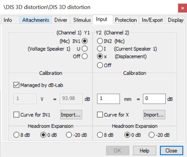
Y1#

Specifies the signal that is acquired on the first channel. IN1 is the signal at the connector as specified in the KA3 Signal Configuration, or the IN1 connector of the Distortion Analyzer hardware (usually a microphone). Us is the voltage at the terminals of the driver connected to the Speaker 1 or Speaker 2 connector. If you choose Off no signal is acquired on channel 1. This way the measurement can be speeded up.

Y2#

Specifies the signal that is acquired on the second channel. IN2 is the signal at the connector as specified in the KA3 Signal Configuration, or at the IN2 connector of the Distortion Analyzer (usually a microphone). Is is the current at the terminals of the driver connected to the Speaker 1 or Speaker 2 connector. X denotes the signal from the laser displacement sensor. If you choose Off, no signal is acquired on channel 2. This way the measurement can be speeded up.

Calibration#

If the check box Managed by dB‑Lab is selected, the selected microphone sensor calibration file is used. You can override a given sensor calibration file by unchecking and setting custom values.

Clicking the Import… opens a dialog where the calibration curve for the corresponding signal can be imported (see section How to Load a Microphone Correction Curve in part 3 of the Tutorial). If a valid curve is imported the button will be labeled Edit… and opens a dialog for editing the calibration curve. For each physical signal (IN1, IN2, \(U_{\text{s}}\), \(I_{\text{s}}\), \(X\)) a separate calibration curve \(H_{Cal}(f)\) can be imported and stored in the database. The measured spectra \(Y_{1}(f)\) , \(Y_{2}(f)\) are divided by the calibration curve

\[Y_{\text{cal}}\left( f \right) = \frac{Y\left( f \right)}{H_{\text{cal}}\left( f \right)}\]

for all signal lines \(f\), if the adjoined check box Curve for is selected. If the check box is not selected, the measured signal is left unchanged. The calibration curve can be used to compensate frequency dependency of the hardware. This way the frequency dependency of the current sensors or of a microphone can be eliminated. Microphone manufacturers usually provide a reference curve that shows the frequency dependency of the microphone. To use that curve as calibration curve transfer it to the clipboard see section How to Load a Microphone Correction Curve in part 3 of the Tutorial and click Import… . Furthermore, the whole signal path can be included in the compensation. For instance, to compensate the current measurement replace the driver by a calibrated resistor. The measured spectrum \(J_{\text{s}}(f)\) can then be used to generate the calibration curve.

Headroom Expansion#

Headroom expansion for first or second channel respectively. The headroom for data acquisition can be increased by 8 dB to cope with very large signals that exceed the normal operational range. To increase the measurement accuracy for very small signals the headroom can be decreased by 20 dB as well.

PROTECTION Page#

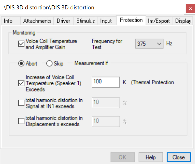
Monitoring: Voice Coil Temperature and Amplifier Gain#

If selected a test measurement is performed after each voltage*frequency sweep point. This way the increase of voice coil temperature and the amplifier gain are monitored. The results of the temperature measurement are shown in result window Delta Tv. Deselecting Monitoring will speed up the measurement.

Frequency for Test Measurement#

The user can choose between three different frequencies for the test measurement. This is quite useful if several drivers are connected via a crossover. In this case a particular driver can be selected for temperature monitoring (e.g. a tweeter) by selecting a test frequency that is in the pass band for the driver.

Abort / Skip#

If Abort is selected the measurement is aborted after one of the protection limits is violated. In case Skip is selected and the protection limits are exceeded for some excitation voltage \(U_1 = U_{\text{lim}}\) then all subsequent sweep points with the same excitation frequency and voltage \(> U_{\text{lim}}\) will be skipped. Skip can only be selected if also Monitoring is selected.

Increase of Voice Coil Temperature Exceeds#

The user can specify an upper limit for the increase of voice coil temperature. In case the adjoined checkbox is activated the measurement is skipped or aborted if the limit is exceeded. This provides a convenient way to protect the driver thermally.

Total Harmonic Distortion Exceeds#

The user can specify an upper limit for total harmonic distortion in the signal acquired on channel 1 or channel 2 respectively. In case the adjoined checkbox is activated the measurement is skipped or aborted if the limit is exceeded. Mechanical malfunction (like voice hitting the back plate) produces harmonic distortion in sound pressure or displacement. Using a limit of say 10 % for those signals the driver can be protected mechanically.

IM/EXPORT Page#

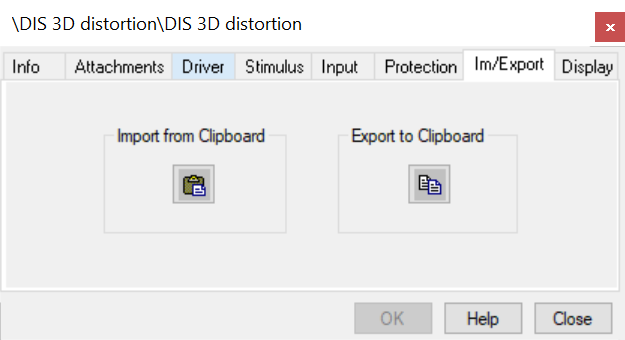
All DIS setup parameters can be imported from and exported to other DIS operations:

Export whole DIS setup to the clipboard

Import whole DIS setup from the clipboard

Furthermore, the stimulus parameters (settings of the voltage-frequency sweep) can be exported to and imported from SIM operations. To do so, press the Export button. Open the SIM operation and press the Import button in property page IM/EXPORT. All setup parameters of interest are now read from the clipboard into the SIM operation.

All modules supporting DIS import and export functionality are documented in the section Supported Modules for Im/Export.

DISPLAY Page#

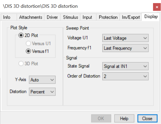
Plot Style: 2D#

If selected all 3D result windows are switched to 2D*mode. The distortion can be plotted either versus excitation voltage \(U_{\text{1}}\) (versus U1) or versus excitation frequency \(f_{\text{1}}\) (versus f1). The windows will be empty if no voltage sweep was performed and versus U1 is selected or if no frequency sweep was performed and versus f1 was selected.

Plot Style: 3D#

If selected the distortion are plotted versus excitation voltage and frequency. The windows will be empty if either no voltage sweep or no frequency sweep was performed.

Plot Style: Y-axis#

This combo box is for adjusting the spacing of the \(y\)‑axis of the result windows

Fundamental
Harmonic (n)
Diff. Intermod (n)
Sum. Intermod (n) and
Peak + Bottom.

First, linear (Lin) or logarithmic (Log) spacing can be chosen. If Auto is selected the spacing is chosen automatically. In order to visualize the effects of power compression, automatic spacing is selected according to the spacing of the voltage sweep selected in property page Stimulus. In case of no power compression simulation results for different drive levels will be displayed as equidistant curves. Any power compression will disturb this equidistant spacing. The \(y\)-axis spacing (Lin/Log/Auto) can be selected independently for signals Y1 and Y2.

Plot Style: Distortion#

This combobox controls the display of the relative harmonic and intermodulation distortion. The relative distortion can be displayed either in Percent or in dB.

Voltage U1#

Determines sweep voltage \(U_{\text{1}}\) for which the results are to be shown in the result windows

Table Components,
Table Signal Characteristics,
Harmonics, % and
Fundamental + Harmonics.

In order not to inflate database size the complete waveform and the according spectra are not stored in the database. However, if you want to view waveform and spectra for a particular sweep point you can repeat the measurement for this single sweep point. After the single point measurement has finished the waveform and spectra for the selected sweep point can be viewed.

Frequency f1#

Determines sweep frequency \(f_{\text{1}}\) for which the results are to be shown in the result windows Table Components and Table Signal Characteristics.

In order not to inflate database size the complete waveform and the according spectra are not stored in the database. However, if you want to view waveform and spectra for a particular sweep point you can repeat the measurement for this single sweep point. After the single point measurement has finished the waveform and spectra for the selected sweep point can be viewed.

State Signal#

Determines the signal (channel) for which the results are to be shown. The user can choose between the two signals (Signal at IN1, Signal at IN2, Voltage at terminals, Current at terminals, Displacement) selected for measurement in property page IMPUT.

Order of Distortion#

Determines the order of distortion (2, 3,…, \(n\)) for which the results are to be shown in result windows

Harmonics (n),
Diff. Intermod (n) and
Sum. Intermod (n).

\(n\) is the Maximal order of distortion analysis specified in property page Stimulus.

Result Windows#

Table Distortion Components#

This result window lists the harmonic and intermodulation distortion components in magnitude and phase as well as the distortion measures for the signal and the sweep point selected in property page DISPLAY.

Table Signal Characteristic#

This result window gives an overview of the properties of the signals measured for the sweep point selected in property page DISPLAY.

Harmonics Distortion#

The second-order harmonic component

\[d_{\text{h2}} = \frac{p\left( 2f \right)}{p_{\text{RMS}}} \cdot 100\%\]

and the third-order harmonic distortion

\[d_{\text{h3}} = \frac{p\left( 3f \right)}{p_{\text{RMS}}} \cdot 100\%\]

are defined in percent where \(p_RMS\) is the true RMS-value of the analyzed signal. The distortion can either be displayed in percent or in dB (0 dB = 100 %). This selection is made in property page DISPLAY.

THD Total Harmonic Distortion#

The IEC standard 60268 defines the total harmonic distortion

\[d_{\text{ht}} = \frac{\sqrt{{p\left( 2f \right)}^{2} + {p\left( 3f \right)}^{2} + \cdots + {p\left( \text{nf} \right)}^{2}}}{p_{\text{RMS}}} \cdot 100\%\]

in percent where \(p_RMS\) is the true RMS-value of the analyzed signal. The distortion can either be displayed in percent or in dB (0 dB = 100 %). This selection is made in property page DISPLAY.

2^nd Harmonic Distortion#

The second-order harmonic component

\[d_{\text{h2}} = \frac{p\left( 2f \right)}{p_{\text{RMS}}} \cdot 100\%\]

is defined in percent where \(p_RMS\) is the true RMS-value of the analyzed signal. The distortion can either be displayed in percent or in dB (0 dB = 100 %). This selection is made in property page DISPLAY.

3^rd Harmonic Distortion#

The third-order harmonic distortion

\[d_{\text{h3}} = \frac{p\left( 3f \right)}{p_{\text{RMS}}} \cdot 100\%\]

is defined in percent where \(p_RMS\) is the true RMS-value of the analyzed signal. The distortion can either be displayed in percent or in dB (0 dB = 100 %). This selection is made in property page DISPLAY.

2^nd Intermodulation Distortion#

The IEC standard 60268 defines the second-order modulation distortion (centered on frequency \(f_{\text{1}}\))

\[d_{\text{2}} = \frac{p\left( f_{1} - f_{2} \right) + p\left( f_{1} + f_{2} \right)}{p\left( f_{1} \right)} \cdot 100\%\]

in percent. If \(f_{\text{1}}\) and \(f_{\text{2}}\) are exchanged in the above formula it defines the second-order modulation distortion centered around frequency \(f_{\text{2}}\). The distortion can either be displayed in percent or in dB (0 dB = 100 %). This selection is made in property page DISPLAY.

3^rd Intermodulation Distortion#

The IEC standard 60268 defines the third-order modulation distortion (centered on frequency \(f_{\text{1}}\))

\[d_{\text{3}} = \frac{p\left( f_{1} - 2f_{2} \right) + p\left( f_{1} + 2f_{2} \right)}{p\left( f_{1} \right)} \cdot 100\%\]

in percent. If \(f_{\text{1}}\) and \(f_{\text{2}}\) are exchanged in the above formula it defines the third-order modulation distortion centered around frequency \(f_{\text{2}}\). The distortion can either be displayed in percent or in dB (0 dB = 100 %). This selection is made in property page DISPLAY.

THDN Total Harmonic Distortion + Noise#

The total harmonic distortion + noise is calculated using the following relationship

\[d_{\text{THDN}} = \frac{\sqrt{p_{\text{RMS}}^{2} - p^{2}\left( f \right)}}{p_{\text{RMS}}} \cdot 100\%\]

The distortion can either be displayed in percent or in dB (0 dB = 100 %). This selection is made in property page DISPLAY.

Modulation#

Note

This Feature is available DIS Pro only.

Excited with a two-tone signal the loudspeaker produces modulation distortion caused by amplitude and phase (frequency) modulation. Both modulations will produce intermodulation components at frequencies \(f_1 - (n-1)\cdot f_2\) and summed-tone intermodulation distortion \(f_1 + (n-1) \cdot f_2\) n^th-order centered around the voice tone \(f_{\text{1}}\).

Assessing Frequency and Amplitude Modulation Distortion#

The IEC standard 60268 defines the 2^nd-order modulation distortion (centered on frequency \(f_{\text{1}}\))

\[d_{\text{2}} = \frac{p\left( f_{1} - f_{2} \right) + p\left( f_{1} + f_{2} \right)}{p\left( f_{1} \right)} \cdot 100\%\]

in percent and the 3^rd-order modulation distortion (centered on frequency \(f_{\text{1}}\))

\[d_{\text{3}} = \frac{p\left( f_{1} - 2f_{2} \right) + p\left( f_{1} + 2f_{2} \right)}{p\left( f_{1} \right)} \cdot 100\%\]

in percent. If \(f_{\text{1}}\) and \(f_{\text{2}}\) are exchanged in the above formulas they define the modulation distortion centered around frequency \(f_{\text{2}}\).

Summarizing the 2^nd and 3^rd-order modulation distortion we get the modulation distortion

\[d_{\text{m}} = d_{\text{2}} + d_{\text{3}}\]

Assessing Amplitude Modulation Only#

The distortion of the pure amplitude modulation can be assessed separately by measuring the variation of the envelope of the high-frequency tone \(f_{\text{1}}\) (voice tone).

The envelope \(E[t]\) of the voice tone \(f_{\text{1}}\) is derived from the time sound pressure signal \(p[t]\) by considering the fundamental of \(f_{\text{1}}\) and the summed-tone and difference-tone intermodulation \(f_1 - (n-1) \cdot f_2\) and \(f_1 + (n-1) \cdot f_2\), respectively, with \(2 < n \in\mathbb{N}\).

Calculating the averaged envelope over one period \(T\)

\[\overline{E} = \frac{1}{T}\int_{0}^{\ }{E\left\lbrack t \right\rbrack\text{dt}}\]

We define the RMS-amplitude modulation distortion

\[d_{\text{AMD}} = \frac{\sqrt{\frac{2}{T}\int_{0}^{\ } {\left( E\left\lbrack t \right\rbrack - \overline{E} \right)^{2}\text{dt}}}}{\overline{E}}\]

The modulation distortion can either be displayed in percent or in dB (0 dB = 100 %). This selection is made in property page DISPLAY.

Fundamental + Harmonics#

The fundamental component

\[L = 20 \cdot \log_{10}\left( \frac{p\left( f_{1} \right)}{p_{\text{ref}}} \right)\]

and the n^th-order harmonic distortion (\(n\)=2,3)

\[L_{\text{hn}} = 20 \cdot \log_{10}\left( \frac{p\left( nf_{1} \right)}{p_{\text{ref}}} \right)\]

of excitation frequency \(f\) is expressed in dB using the dB reference value \(p_ref\). \(p_ref\) is calculated using the calibration settings specified in property page INPUT.

Weighted Harmonics (HI-2)#

The DIS-PRO version records the fundamental and the first through tenth harmonics \(p(k\cdot f)\) with \(0 < k < 11\). The harmonics are weighted by 12 dB per octave rising with frequency relative to the level of the fourth harmonic by using the weighting function

\[w\left( k \right) = S^{\log_{2}\left( \frac{k}{R} \right)}\]

depending on the order \(k\), using the slope parameter \(S= 4\cdot (12\text{db}/\text{octave})\) and the referenced harmonic \(R=4\). The HI-2 distortion is the rms-sum of the weighted harmonic

\[L_{\text{HI-2}} = 10 \cdot \log_{10}\left( \frac{\sum_{k = 2}^{K}\left( w\left( k \right) \cdot p\left( \text{kf} \right) \right)^{2}}{p_{\text{ref}}^{2}} \right)\]

The reference amplitude \(p_ref\) is the set to the mean amplitude of the fundamental component in the pass band of the driver.

Please find more information in the application note AN7 Measurement of Weighted Harmonic Distortion Hi-2.

Mtop, Mbottom (IMD)#

The PRO version of the DIS measures the amplitude modulation (called IMD in automotive application) by assessing the variation of the envelope of the high-frequency tone \(f_{\text{1}}\) (voice tone) versus one period of the low-frequency tone \(f_{\text{2}}\).

The envelope \(E[t]\) of the voice tone \(f_{\text{1}}\) is derived from the sound pressure signal \(p[t]\) by considering the fundamental of \(f_{\text{1}}\) and the summed-tone and difference-tone intermodulation \(f+(n-1)\cdot f_2\) and \(f_1-(n-1)\cdot f_2\) respectively, with \(2 < n < N\).

If the envelope \(E[t]\) is constant over the period \(T=1/f_2\) then the high frequency tone is not amplitude modulated. Frequency modulation caused by the Doppler effect will cause no variation of the envelope \(E[t]\) versus \(t\).

The maximal value of the envelope \(E[t]\) over one period T is called top modulation

\[E_{\text{top}} = 20 \cdot \log_{10}{\max_{t \leq t + T}\left( E\left\lbrack t \right\rbrack \right)}\]

The minimal value of the envelope \(E[t]\) over one period T is called bottom modulation

\[E_{\text{bottom}} = 20 \cdot \log_{10}{\min_{t \leq t + T}\left( E\left\lbrack t \right\rbrack \right)}\]

The Top modulation \(M_{\text{Top}}\) is determined by comparing the maximum of the envelope \(E_{\text{top}}\) with the amplitude response \(L_{f_1}\) of the reference measurement (without bass tone)

\[M_{\text{top}}\left( f_{1} \right) = E_{\text{top}}\left( f_{1} \right) - L_{\text{1}}\left( f_{1} \right)\]

The Bottom modulation \(M_{\text{Bottom}}\) is determined by comparing the minimum of the envelope \(E_{\text{bottom}}\) with the amplitude response \(L_{f_1}\) of the reference measurement (without bass tone)

\[M_{\text{bottom}}\left( f_{1} \right) = E_{\text{bottom}}\left( f_{1} \right) - L_{\text{1}}\left( f_{1} \right)\]

Please find more information in the application note AN6 Measurement of Amplitude Modulation.

Fundamental#

This result window shows the fundamental component versus frequency \(f_{\text{1}}\) and/or voltage \(U_{\text{1}}\) for the signal selected in property page DISPLAY. The fundamental can either be displayed linearly in real physical units or logarithmically in dB.

\[L = 20 \cdot \log_{10}\left( \frac{p\left( f_{1} \right)}{p_{\text{ref}}} \right)\]

This selection is made in property page DISPLAY (see section Linear / dB y‑axis of Result Windows in part 3 of Tutorial). The dB reference value \(p_ref\) calculated using the calibration settings specified in property page INPUT.

Calibration Curves#

The window shows the calibration curves \(H_{\text{Cal1}}(f)\) and \(H_{\text{Cal2}}(f)\). The spectrum of the signal measured on channel 1 and channel 2 is corrected with \(H_{\text{Cal1}}(f)\) and \(H_{\text{Cal2}}(f)\), respectively (see section INPUT page Calibration for …).

Compression#

The compression of the amplitude of fundamental component at sweep frequency \(f_{\text{1}}\) and sweep voltage \(U_{\text{1}}\) is defined by

\[C = 20 \cdot \log_{10}\left( \frac{p\left( f_{1} \right) \cdot U_{\text{start}}}{U_{\text{1}}} \right)\]

where \(U_{\text{start}}\) is the starting value of the voltage sweep.

Absolute Harmonic Components#

This result window shows the n^th-order harmonic distortion component versus frequency \(f_{\text{1}}\) and/or voltage \(U_{\text{1}}\) for the signal selected in the property page DISPLAY.

The harmonic distortion component can either be displayed linearly in real physical units or logarithmically in dB

\[L_{\text{hn}} = 20 \cdot \log_{10}\left( \frac{p\left( nf_{1} \right)}{p_{\text{ref}}} \right)\]

This selection is made in property page DISPLAY (see section Linear / dB y‑axis of Result Windows in part 3 of Tutorial). The dB reference value \(p_ref\) calculated using the calibration settings specified in property page INPUT.

Difference Intermodulation#

This result window shows the n^th-order difference-tone intermodulation component (\(n=2,3,\ldots\)) versus frequency \(f_{\text{1}}\) and/or voltage \(U_{\text{1}}\) for the signal and the order \(n\) selected in property page DISPLAY. The intermodulation components are centered on frequency \(f_{\text{1}}\).

The intermodulation component can either be displayed linearly in real physical units or logarithmically in dB

\[L = 20 \cdot \log_{10}\left( \frac{p\left( f_{1} - \left\lbrack n - 1 \right\rbrack \cdot f_{2} \right)} {p_{\text{ref}}} \right)\]

This selection is made in property page DISPLAY (see section Linear / dB y‑axis of Result Windows in part 3 of Tutorial). The dB reference value \(p_ref\) calculated using the calibration settings specified in property page INPUT.

Summed Intermodulation#

This result window shows the n^th-order summed-tone intermodulation component (\(n\) # 2, 3, …) versus frequency \(f_{\text{1}}\) and/or voltage \(U_{\text{1}}\) for the signal and the order \(n\) selected in the property page DISPLAY. The intermodulation components are centered around frequency \(f_{\text{1}}\).

The intermodulation component can either be displayed linearly in real physical units or logarithmically in dB

\[L = 20 \cdot \log_{10}\left( \frac{p\left( f_{1} + \left\lbrack n - 1 \right\rbrack \cdot f_{2} \right)}{p_{\text{ref}}} \right)\]

This selection is made in property page DISPLAY (see section Linear / dB y‑axis of Result Windows in part 3 of Tutorial). The dB reference value \(p_ref\) calculated using the calibration settings specified in property page INPUT.

DC Component#

This result window shows the DC component versus \(f_{\text{1}}\) and/or voltage \(U_{\text{1}}\) for the signal selected in property page DISPLAY. It will be determined by the lowest FFT frequency line, which represents the DC component of the measured signal. It will not be displayed at the spectrum result windows, showing only AC components.

Peak + Bottom#

The result window presents the minimal and maximal values versus frequency \(f_{\text{1}}\) and/or voltage \(U_{\text{1}}\) for the signal selected in property page DISPLAY.

The results can either be displayed linearly in real physical units or logarithmically in dB. This selection is made in property page DISPLAY (see section Linear / dB y‑axis of Result Windows in part 3 of Tutorial). As the result window shows both min and max values it cannot be switched to the 3D display mode.

\(\triangle T_{\text{V}}(t)\) Temperature#

The increase of the voice coil temperature \(\Delta\) \(T_{\text{V}}\) is displayed versus frequency \(f_{\text{1}}\) and/or voltage \(U_{\text{1}}\).

y1(t) Input Waveform#

After pausing or finishing the measurement the window shows the waveform of the signal acquired on channel 1 (see section How to View Waveforms and Spectra? in part 3 of the Tutorial).

y2(t) Input Waveform#

After pausing or finishing the measurement the window shows the waveform of the signal acquired on channel 2 (see section How to View Waveforms and Spectra? in part 3 of the Tutorial).

Y1(f) Input Spectrum#

After pausing or finishing the measurement the window shows the spectrum of the signal acquired on channel 1 (see section How to View Waveforms and Spectra? in part 3 of the Tutorial).

Y2(f) Input Spectrum#

After pausing or finishing the measurement the window shows the spectrum of the signal acquired on channel 2 (see section How to View Waveforms and Spectra? in part 3 of the Tutorial).

Supported Modules for Im/Export#

Malfunction and Troubleshooting#

Overview#

This chapter will provide information that can help you solve common problems that occur with the Distortion Analyzer and the DIS module. The software generates a variety of warnings automatically if the signals are badly conditioned or a malfunction state is detected. Some information may be neglected but it is always recommended to find out the cause of the problem.

If you cannot find a description here that matches your problem, try these options:

Check the Malfunction and Troubleshooting section of the dB-Lab documentation.

Check the file readme.txt that you received with your Distortion Analyzer products. This document contains the most up-to-date information.

Contact us via support

Error and Warning Messages#

Primary data is already available#

Measurement results will be deleted if the corresponding setup parameters are changed. This way results and setup parameter are kept consistent. If you want to perform a new measurement while preserving the old results, please create a new operation. The setup parameters of the old measurement can be conveniently copied to new operation with the Copy and Paste buttons that you find on property page IM/EXPORT (see above).

WARNING: Stimulus is applied to OUT 1#

This warning will be generated if Voltage: at OUT1 is selected in property page STIMULUS. In this case the stimulus voltage specified in property page STIMULUS is the voltage at the output connector OUT 1. If an amplifier is used this voltage is the voltage at the amplifier input. The level of the amplifier output signal can be considerably higher than the specified level and can possibly destroy your speaker! Please make sure that no amplifier is connected if you select Voltage: at OUT1.

No proper amplifier output#

Cause:: The DIS tests the amplifier before the main measurement. If the amplifier is switched off or if the test signal is not transmitted properly (e.g. low amplifier gain or insufficient SNR), this error occurs.
Remedy:: Check the amplifier. Increase the amplifier gain. Check the connection and the cables in the hardware setup. Is the amplifier input connected to OUT1? Is speaker cable connected to the speaker output specified in property page STIMULUS?

Desired voltage sweep cannot be realized#

Cause:: This error message occurs if no amplifier is used (selection Voltage: at OUT1 in property page STIMULUS) and the desires excitation level at output connector OUT 1 is too high to be realized.
Remedy:: Decrease excitation level to the value shown in the message box. Alternatively use an amplifier.

Significant amplifier distortions#

Cause:: The amplifier is tested before the main measurement is started. The error message is generated if the amplifier produces significant distortion during this test. Limiting of the amplifier is one possible reason
Remedy:: Check the amplifier. If the amplifier is limiting reduce the sweep voltage Uend in property page STIMULUS or use a more powerful amplifier.

Output calibration factor out of range#

This error message occurs if the hardware device is severely de*calibrated. This is a serious problem. Please stop running measurements and contact your local dealer or the KLIPPEL support.

Amplifier gain has changed considerably#

The gain of the amplifier is measured before the voltage/frequency sweep is started. During the sweep a constant amplifier gain is assumed. If the gain is changed during the sweep the measurement stops with the above error message. If using a KA3 this error can also be caused if the sense clamps of the DUT speaker cable are not connected.

Single point measurement failed#

This error message is generated if single point measurement was performed after changing the frequencies \(f_{\text{start}}\), \(f_{\text{end}}\) or the voltages \(U_{\text{start}}\), \(U_{\text{end}}\) of the sweep. The results of the single point measurement cannot be match to the previous results in this case. This error will not occur if you use a recent version of the DIS module.

Increase of voice coil temperature exceeds the limit#

The increase of the voice coil temperature during the measurement exceeds the limit specified for thermal protection in property page PROTECTION. The measurement will be aborted. If you don’t want to protect your driver, switch off thermal protection in property page PROTECTION.

Total harmonic distortion for Y1 exceeds the limit#

The total harmonic distortion in the input signal Y1 (channel 1) exceeds the limit specified for protection in property page PROTECTION. The measurement will be aborted. If you don’t want to protect your driver switch off THD protection in property page PROTECTION.

Total harmonic distortion for Y2 exceeds the limit#

The total harmonic distortion in the input signal Y2 (channel 2) exceeds the limit specified for protection in property page PROTECTION. The measurement will be aborted. If you don’t want to protect your driver switch off THD protection in property PROTECTION.

Signal Y1 is limiting#

Cause:: The signal acquired on input channel 1 is limiting. You can either stop or proceed the measurement.
Remedy:: Increase Headroom Expansion for (Channel 1) Y1 to 8 dB in property page INPUT to 8dB. Alternatively, you can decrease the sweep voltage Uend in property page STIMULUS.

Signal Y2 is limiting#

Cause:: The signal acquired on input channel 2 is limiting. You can either stop or proceed the measurement.
Remedy:: Increase Headroom expansion for (Channel 2) Y2 to 8 dB in property page INPUT. Alternatively, you can decrease the sweep voltage Uend in property page STIMULUS.

High Sensitivity current sensor selected#

High Sensitivity current sensor selected: Voltage at the DUT (speaker) could be lower than specified, due to the used shunt resistor.

Cause:: The current sensing shunt resistor used to get the best possible SNR in the current signal is placed in series to the DUT. Depending on the DUT’s impedance the shunt resistor causes a frequency depending voltage reduction at the DUT.
Remedy:: Select the Low Sensitivity hall effect current sensor, in KA3 / Signal Configuration if voltage reduction should be avoided.

Note

This warning is displayed for KA3 hardware only. It indicates a possible voltage drop due to the current sense resistor. Therefore, the specified voltage may not be realized. See also section Difference between specified and applied voltage.

Further problems#

Difference between specified and applied voltage#

The excitation voltage specified in property page STIMULUS and the voltage applied to the speaker terminals differ slightly. The amplifier gain is measured for the frequency specified in group Monitoring in property page PROTECTION. For safety reasons the driver is disconnected during the gain measurement. Voltage at the amplifier output changes slightly for other frequencies and due to the load of the driver. If you are interested in the exact value of the voltage applied to the driver you can choose the terminal voltage as one of the input signals (select (Voltage Speaker 1) Us in property page INPUT).

Difference between specified and applied frequency#

The stimulus signal of the DIS module is kept synchronous to the FFT size. This way windowing can be omitted while avoiding any smearing effects due to spectral leakage. However, this implies that only frequencies can be used that are multiples of \(\Delta f = f_{\text{sample}} / n\), where \(n\) is the signal length. The program automatically maps all frequencies specified by the user to the closest multiple of \(\triangle f\). The mapped frequencies are used in all result charts and tables. You can check the mapped excitation frequencies \(f_{\text{1}}\) and \(f_{\text{2}}\) in Table Signal Characteristics and Table Components. The Frequencies \(f_{\text{1}}\) and \(f_{\text{2}}\) are mapped very close to the specified values if Frequency f1 Sweep is switched off in property page STIMULUS. If Mode: Harmonics is selected in property page STIMULUS and Monitoring is switched off in property page PROTECTION a DFT algorithm is used instead of a FFT algorithm leading to very close mapping as well.

DIS – Distortion

On this page

DIS – Distortion#

Overview#

DIS Tutorial#

Viewing DIS Results (Part 1)#

Measurement Results#

Performing a new DIS (part 2)#

Requirements#

Connect Hardware#

Creating a New Operation#

Setup Data#

Measurement Setup#

Display Setup#

Start Measurement#

Viewing and checking results#

Customizing DIS (part 3)#

How to Protect Drivers#

How to Protect Drivers Connected to a Crossover#

Speed up Measurement#

How to calibrate sensors?#

How to Load a Microphone Correction Curve?#

Example#

How to Load Correction Curves for Other Input Signals?#

How to Cope With Time Delay?#

How to Cope With Creep?#

How to View Waveforms and Spectra?#

How to Copy Stimulus Settings From or To SIM#

Nominal Versus Measured Voltage#

How to Switch 2D / 3D#

Linear / dB y‑axis of Result Windows#

Add Comments#

DIS Reference#

Measurement Technique#

Signal Generation#

Excitation#

Frequency Sweep#

Voltage Sweep#

Measurement Modes#

Measurement of Harmonics#

Measurement of Intermodulations#

Measurement of Total Harmonics + Noise#

Post Processing#

Property Pages#

INFO Page#

DRIVER Page#

STIMULUS Page#

Mode#

Voltage U1#

Voltage U1: at Speaker Terminals#

Voltage U1: at OUT 1#

Voltage: U2/U1#

Frequency f1#

Frequency f2#

Maximum Order of Distortion Analysis#

Additional Excitation Before Measurement#

Minimum Silence Between Steps#

Device Measurement Capabilities#

INPUT Page#

Y1#

Y2#

Calibration#

Headroom Expansion#

PROTECTION Page#

Monitoring: Voice Coil Temperature and Amplifier Gain#

Frequency for Test Measurement#

Abort / Skip#

Increase of Voice Coil Temperature Exceeds#

Total Harmonic Distortion Exceeds#

IM/EXPORT Page#

DISPLAY Page#

Plot Style: 2D#

Plot Style: 3D#

Plot Style: Y-axis#

Plot Style: Distortion#

Voltage U1#

Frequency f1#

State Signal#

Order of Distortion#

Result Windows#

2^nd Harmonic Distortion#

3^rd Harmonic Distortion#

2^nd Intermodulation Distortion#

3^rd Intermodulation Distortion#