PPP – Programmable Post-Processing

PPP - Tutorial

Overview

The PPP module is built for any user-defined post-processing within dB-Lab. The curves and single values may be either entered manually or imported from any other dB-Lab operation within the same dB-Lab object. It’s also possible to export the calculated results to the setup of other dB-Lab operations.

Getting started

This chapter shows some examples which should simplify the understanding what is possible with the PPP module. Each of these examples could be found in the example database in dB-Lab (210 or higher).

Example 1: Post-process Temp.-Coefficient for LSI

The LSI and PWT measurements are using pre-defined temperature coefficients for the temperature calculation out of the measured Re values. If you are using a very special voice coil material with other temperature coefficient than that of copper or aluminum then you may use the PPP module for re-calculating the temperature curve.

Therefore, the measured Re curve can be automatically imported from the LSI (or PWT) measurement and processed in the PPP operation.

Here is a short step-by-step instruction how to set the properties of the PPP module for this application:

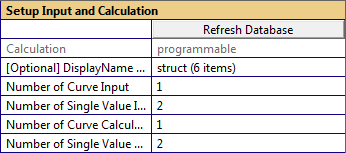
1. In the first category at property page Input you have to define the number of curve and single value inputs as well as the number of calculations. All following categories in the UI will be shown accordingly.

   For this example you need 1 curve input (the Re curve of the LSI measurement), 2 single values (the new temperature coefficient and the reference resistance) and several calculations (see below).

   
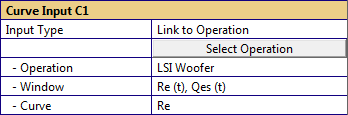
2. The first curve input is used to import the measured Re curve from the LSI measurement. Therefor the Input Type is set to Link to Operation and the parameters Operation, Window and Curve are set accordingly.

   
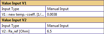
3. Both single value inputs are used as manual inputs of constants. Therefor both input types are set to Manual Input. You may enter any value here that corresponds to your application.

   
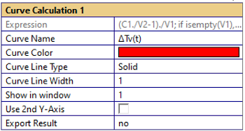
4. The curve calculation at property page Processing calculates the new temperature curve from the imported Re curve regarding the new temperature coefficient and the reference resistance. The equation for the calculation is as follows:
   \[\mathrm{\Delta}T = \frac{\frac{\text{Re}\left( t \right)}{R_{\text{ref}}} - 1}{\alpha}\]
   This curve will be shown in window 1 without exporting it to any other operation.
   
5. Both single value calculations are used to show the two user inputs (reference resistance and temperature coefficient) in the result table for better visualization.

   
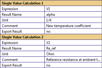
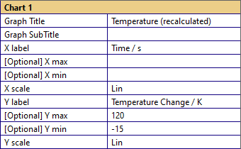
6. The property page Display is used for setting up the properties of the graph result window. The parameters in this section should be self-explanatory.

   

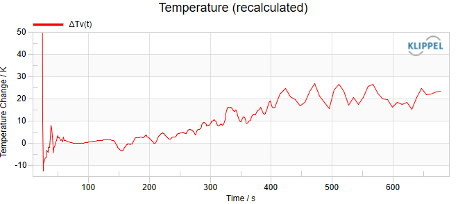
The result window of this example looks like the following:

Example 2: Measurement at defined terminal voltage

Using very long cables between KLIPPEL Analyzer Hardware and the DUT may cause non-constant stimulus voltage at the DUT’s terminals due to the resistance of the cable and the impedance of the DUT (even if 4-wire connection is used). To compensate for this fact, you may shape the stimulus voltage at the output of the measurement device so that it’s constant at the DUT’s terminals. This measurement application is described in the Application Note 41: Measurement at defined terminal voltage accordingly.

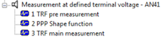
The PPP module is used in this case as the interface between a pre-measurement and the main measurement. The pre-measurement is used to measure the frequency dependent transfer function between the output of the KLIPPEL Analyzer Hardware and DUT’s terminals. From this transfer function the final stimulus shaping will be calculated using the PPP module. Finally, the calculated shaping curve will be sent to the main measurement.

All curves and single values are imported and exported between the different operations automatically, so nothing has to be copied manually.

Here is a short step-by-step instruction how to set up the properties of the PPP module for this application:

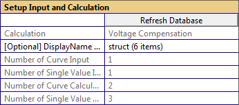
1. In the first category you have to define the number of curve and single value inputs as well as the number of calculations. All following categories in the UI will be shown accordingly.

   For this example you need 1 curve input (the transfer function of the pre-measurement), 1 single value (the stimulus voltage of the pre-measurement) and several calculations (see below).

   
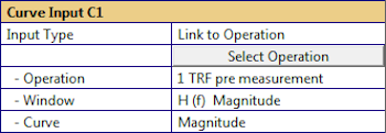
2. The first curve input is used to import the transfer function between KLIPPEL Analyzer hardware and the speaker terminals from the pre-measurement. Therefor the Input Type is set to Link to Operation and the parameters Operation, Window and Curve are set accordingly.

   
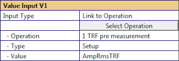
3. The single value input is used to import the stimulus voltage of the pre-measurement. This information is needed for setting the stimulus voltage of the main measurement correctly.

   Selecting the single value works in the same way as selecting the curve inputs. For the single values you have to choose whether you want to import a Setup or a Result value. In this case we are using the type Setup because the stimulus voltage belongs to the setup.

   
4. The first curve calculation only shows the imported curve from the pre-measurement for reference. The Expression in this case is simply “C1” because you only want to show the curve C1 without any post-processing.

   This curve will be shown in window 1 without exporting it to any other operation.

   
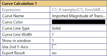
5. The second curve calculation is used for calculating the stimulus shaping curve for the main measurement. It will also be shown in result window 1 besides to the original transfer function.

   Since this curve should be used as stimulus shaping in the main measurement it will be automatically exported via the parameter Export Result. The checkbox keep original Operation is not checked because there is no need for a backup of this operation before changing its setup.

   
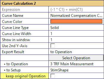
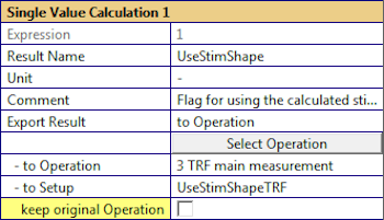
6. The first single value calculation is used to automatically enable the stimulus shaping in the main measurement. Therefor the Expression is simply 1 because it should always be ON independent on any input parameter. The checkbox keep original Operation is disabled again.

   
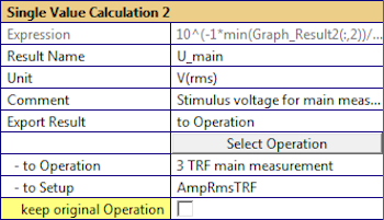
7. The second single value calculation calculates the new stimulus voltage for the main measurement. Due to the fact that the stimulus shaping can only attenuate, the stimulus voltage has to be increased by the amount of attenuation. Again, the new stimulus voltage is exported to the setup of the main measurement automatically.

   
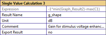
8. This calculation is only for getting a fast overview about the stimulus voltage enhancement between the pre-measurement and the main measurement. It’s more or less an indicator for the cable losses (which also depends on the relation between the DUT impedance and the output impedance of the amplifier). This calculation result will only be shown in the result table and not exported to any other dB-Lab operation.

   
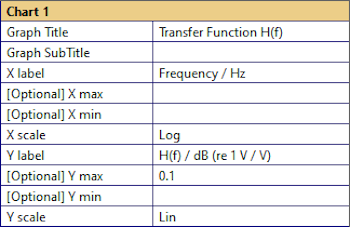
9. The property page Display is used for setting up the properties of the graph result window (both curves are shown in the same graph window). The parameters in this section should be self-explanatory.

   

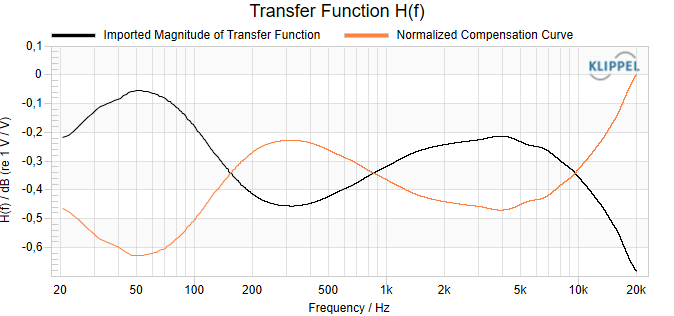
The result window of the PPP operation looks like the following picture. The Normalized Compensation Curve will be automatically exported to the main TRF measurement.

Note

This example is available as free object template in dB-Lab (210.226 or higher) without the need of a valid PPP license.

PPP – Reference

Property Pages

Select the PPP operation in the project window, and click the View properties button. The Property Pages contain the setup parameters and allow import and export of setup parameters and results.

Here is a short summary on the Property Pages and Setup-Categories:

Info

The Info page allows the user to change the name of the measurement and to add a comment to the measurement.

For details, see the dB-Lab Manual.

Input

This property page contains all parameters for setting up the different inputs of the PPP module.

Category: Setup Input and Calculation

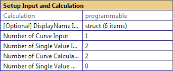
This is the first category that will be shown when creating a new PPP operation in dB-Lab. Here you have to define how many input curves and single values should be available for this operation. Additionally, the number of calculations (results) has to be entered.

The input parameters for the different inputs and calculations will be shown (or hidden) accordingly.

Calculation

This parameter shows the currently defined calculation within the PPP operation. There are some special applications which are coming with the PPP with pre-defined SciLab expressions. You will find a list of these applications in section Programming with the PPP.

Default is “programmable” which means that all expressions have to be user-defined.

DisplayName Input (Optional)

This parameter is used to change the display name of input variables for better visualization. For ex. C1 = ‘TRF’ will change the display name of the input parameter C1 to C1: TRF.

Number of Curve Input

Specify the number of input curves.

Number of Single Value Input

Specify the number of single value inputs.

Number of Curve Calculation

Specify the number of curve calculation results.

Number of Single Value Calculation

Specify the number of Single value calculation results.

Category: Curve Input C1 … C4

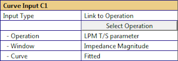
These categories provide all necessary parameters for manual or automatic input of the curve information which should be processed.

Input Type

Choose either “Manual Input” or “Link to Operation”. In case of “Link to Operation” the following 3 parameters will be shown for the automatic link.

• Operation

  Click the button “Select Operation” for choosing the desired dB-Lab operation for automated import. Otherwise you may also enter the name of the dB-Lab operation manually.

• Window

  Choose the desired window within the chosen operation.

• Curve

  Choose the desired curve within the chosen window.

C1 … C4

Manual curve input. possible formats are:

• Real Value

  \[\begin{split}\begin{bmatrix} f_{1} & a_{1} \\ \vdots & \vdots \\ f_{n} & a_{n} \\ \end{bmatrix}\end{split}\]

• Complex Value

  \[\begin{split}\ \begin{bmatrix} f_{1} & a_{1} & \varphi_{1} \\ \vdots & \vdots & \vdots \\ f_{n} & a_{n} & \varphi_{n} \\ \end{bmatrix}\end{split}\]

• with

  • \(f\) … Argument vector (frequency / displacement / voltage / etc.)

  • \(a\) … Amplitude vector (e.g. SPL)

  • \(\varphi\) … Phase vector [Degree]

If you are not familiar with the curve format you can either look to the dB-Lab manual or simply copy a curve from any other dB-Lab operation and paste it manually into the PPP via the Manual Input option. This way you can directly see the format of the pasted curve.

In case of importing curves from a TRF operation there is a special option when selecting the Window. Since the TRF offers some curves in full resolution (e.g. the impulse response) via the property page Im/Export those curves can be found also in the PPP when selecting the window TRF Export Curves.

As inherited property of this module the input curves are interpolated to generate common base points for the different input curves (see category Processing below). Additionally, complex input curves will be converted to complex format with real and imaginary part (e.g. 3+1*i).

Category: Value Input V1 … V2

Same as for the category Curve Input.

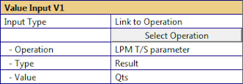
Input Type

Choose either “Manual Input” or “Link to Operation”. In case of “Link to Operation” the following 3 parameters will be shown for the automatic link.

• Operation

  Click the button “Select Operation” for choosing the desired dB-Lab operation for automated import. Otherwise you may also enter the name of the dB-Lab operation manually.

• Type

  Choose whether you want to import a result or a setup parameter from the chosen operation.

• Value

  Choose the desired setup or result parameter.

V1 … V2

Manual single value input.

Processing

Category: Processing

This category contains the selection of the interpolation method which is used to interpolate the input curve data in case of multiple input curves. You have to define whether the input curves have:

• Linear X- and Y-Axis (e.g. time signals)

• Logarithmic X-axis and Linear Y-Axis (e.g. linear voltage signal vs. logarithmic frequency)

• Linear X-Axis and Logarithmic Y-Axis

• Logarithmic X- and Y-Axis (e.g. SPL in dB vs. logarithmic frequency)

Note

The chosen interpolation method is used for all input curves. So, when trying to import multiple curves with different X- or Y-Axis data, you might run into problems.

Category: Curve Calculation 1 … 3

These categories provide the parameters for the post-processing calculations and settings for the result curves. The export of the result curves can also be configured here.

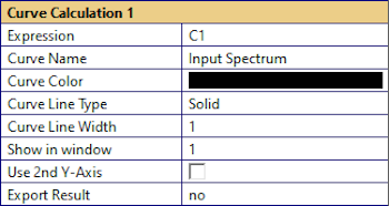
Expression

Any valid SciLab expression as single string or multi-line string could be used for calculation. When using multi-line strings, each line has to be terminated by a semicolon “;”. No equal sign “=” is required within the first line of the expression.

The result must be a 1 or 2 column vector of y-axis values.

• column 1: real part of calculation result

• column 2: imaginary part (optional)

The x-axis information will be automatically extracted from the input curves and is available as the interpolated X-axis of all input curves in the variable X.

Curve Name

Name of the curve that will be shown in the dB-Lab graph window.

Curve Color

Color of the result curve.

Curve Line Type

Type of the result curve. The following options are available:

solid, dashed, dotted, dash-dot & dash-dot-dot

Curve Line Width

Defines the thickness of the result curve

Show in Window

Choose whether the result curve should be shown in graph window 1, 2 or 3. Multiple result curves could be shown in the same graph window.

Use 2^nd Y-Axis

Choose whether you want to show this result curve on the 2^nd Y-Axis in this specific chart. This might be helpful when showing curves with different physical units within the same chart.

Export Result

Choose whether you want to export the calculation result to the setup of another dB-Lab operation. If errors occurred during the calculation, export won’t be done.

• to Operation

  Click the button “Select Operation” for choosing the desired dB-Lab operation for automated export. Otherwise you may also enter the name of the dB-Lab operation manually.

• to Setup

  Choose the desired setup value for automated export.

keep original Operation

Default ON. Normally the chosen dB-Lab operation will be copied before exporting to it because changing a setup parameter within a dB-Lab operation will delete existing measurement results.

Uncheck this box only if you are sure that the operation, which should be used for export, does not contain measurement results or if you change only display parameters (which does not delete results).

All input curves and single values are available with their short names (C1, C2, …, V1, V2) as variables in the SciLab expression. Those variables contain only the complex y-axis information since the x-axis information is available in the separate variable X.

Using separate X-axes for each curve calculation result is possible using the variable X_Result1…3. So, in this case you want to plot the second result curve over a special X-Axis which doesn’t fit the common X-axis, you would have to overwrite the variable X_Result2.

In case of using the 2^nd y-axis the curve color of this curve will be used as the color for the 2^nd y-axis.

Exporting the calculation results is only possible to the setup of other dB-Lab operations within the same dB-Lab object. It is not possible to export the result curves of the PPP operation to any chart of another dB-Lab operation.

Category: Single Value Calculation 1 … 3

In these categories the single value calculations and result visualization can be configured. The single value results may also be exported to the setup of other dB-Lab operations.

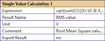
Expression

Any valid SciLab expression as single string or multi-line string that will be used for calculation. When using multi-line strings, each line has to be terminated by a semicolon “;”. No equal sign “=” is required within the first line of the expression.

The calculation result must be a single value (may be complex) or a string.

All variables known from the curve calculation are also available here.

Result Name

Name of the result variable that will be shown in the result table of this operation.

Unit

Unit of the result variable that will be shown in the result table of this operation.

Comment

Any comment that will be shown in the result table of this operation.

Export Result

Same as for Curve Calculation (see above).

• to Operation

  Same as for Curve Calculation (see above).

• to Setup

  Same as for Curve Calculation (see above).

keep original Operation

Same as for Curve Calculation (see above).

Display

Category: Chart 1 … 3

These categories provide all parameters that are necessary for configuration of the result windows. The result windows that are not used will be hidden. Additionally, the parameters for configuration of the 2^nd Y-Axis will be hidden as long as there is no result curve which uses it.

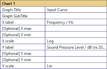
Graph Title

Title of the graph window within dB-Lab.

Graph Sub Title

Subtitle of the graph window within dB-Lab.

X label

Any string that will be shown as label at the X-axis of the graph.

[Optional] X max

Maximum value of the X-axis.

[Optional] X min

Minimum value of the X-axis.

X scale

Choose either linear or logarithmic scaling of the X-axis. Note that logarithmic scaling could not be achieved if X-axis contains values ≤ 0.

Y label

Any string that will be shown as label at the 1^st Y-axis of the graph.

[Optional] Y max

Maximum value of the 1^st Y-axis.

[Optional] Y min

Minimum value of the 1^st Y-axis.

Y scale

Choose either linear or logarithmic scaling of the Y-axis. Note that logarithmic scaling could not be achieved if Y-axis contains values ≤ 0.

2^nd Y label

Same as for the 1^st Y-Axis.

[Optional] 2^nd Y max

Same as for the 1^st Y-Axis.

[Optional] 2^nd Y min

Same as for the 1^st Y-Axis.

2^nd Y scale

Same as for the 1^st Y-Axis.

Im/Export

This property page allows the user to export the whole setup of the PPP operation to the clipboard. This can be used to easily copy the setup to another PPP operation (maybe in another dB-Lab database). In the other operation the setup can be imported from the clipboard as well.

Results

Result Curve 1 … 3

Plots the result obtained from curve calculations 1…3. Each result curve can be renamed and shown in any graph window independently. Additionally, it is possible to use 2 independent Y-Axes in the same chart (e.g. for showing a magnitude [dB] and phase response [degree] in the same chart).

Note

Since dB-Lab can show only two-dimensional curves (only one x-axis and y-axis) any calculated curves containing 3 columns (such as magnitude and phase response in the same curve) will be shown as magnitude response (2^nd column) only! The 3^rd column will not be shown but can be obtained via the manual or automatic export of the PPP module.

Result Table

In the Result Table all results of each single value calculation are shown in a table. All errors and warnings will be shown in this window, too.

Export

Every result curve and single value can be exported in two ways.

1. Clipboard export: Go to property page “Im/Export” of the PPP operation and press the “Export to Clipboard” button. Now the clipboard contains the whole setup and result parameters of the corresponding PPP operation. Simply select the necessary result parameter and copy it wherever you want.

2. Automatic export: It is possible export the calculation results of the PPP operation to the setup of any other dB-Lab operation within the same dB-Lab object. This could easily be used to change for example the stimulus voltage of the next TRF operation which should be performed. Please see the below section for Details how to setup your PPP for automatic export.

Note

Changing the setup of any dB-Lab operation may delete measurement results in this operation!

Automatic Import / Export

This module uses the KLIPPEL Automation Interface for getting and setting the curves and single values from and to other dB-Lab operations. Since the KLIPPEL Automation Interface is also available from other programming languages (e.g. Python, C#, Java) you may also create your own post-processing or automated measurement report, etc.

Please refer to the KLIPPEL Automation Documentation which could be found on the software CD that comes with your KLIPPEL system.

Programming with the PPP

When using the Default PPP operation template in dB-Lab you will get the PPP operation in “programmable” mode which allows you to edit all the SciLab expressions. For running this programmable PPP operation you will need a valid PPP license.

In general, the following variables are available in each expression for processing:

C1 … C4

Containing the interpolated y-axis information of the input curves. Thus, all curves have the same number of rows (they can easily be processed together because they contain equal base points). The X-axis information of all curves will be available as separate variable X and will not be part of the curves C1 … C4.

In case of 3 columns in the curve inputs (assuming 2^nd column as magnitude and 3^rd column as phase information) the input curve will automatically be converted to REAL and IMAGINARY part. Those variables C1 … C4 contain complex values in this case.

V1, V2

Containing the single values that where defined as inputs of the PPP.

X

The x-axis information of all input curves (the 1^st column of each curve) will be used to interpolate all input curves to contain the exact same base points. This is to ensure that all curves can be processed without SciLab error due to different number of rows.

The interpolated x-axis is available as separate variable X and is not part of the variables C1 … C4.

Each of those variables may be used in all the curve and single value calculations.

The output format of the calculation expressions is defined as follows:

• Curve Calculation:

  The calculation result should be a 1 or 2 column vector of the same length as the interpolated x-axis. Since it will be merged together with the interpolated x-axis automatically it doesn’t need to contain any x-axis information. In case of complex (real and imaginary part) values in the calculation result, only the absolute value of the complex vector will be plotted in the chart in dB-Lab. However, the complex values will be available in the curve export over clipboard or the automatic export into another dB-Lab operation (please see the sections above). In case of a 2-column vector in the calculation result (assuming 1^st column as magnitude and 2^nd column as phase information), only the 1^st column will be shown in the dB-Lab chart. The export over clipboard and into another dB-Lab operation will contain all columns.

• Single Value Calculation:

  There are only single row, single column results of scalar or string type allowed as single value results. Thus, it’s not possible showing any matrices as single value result. Complex result values (real and imaginary part) are allowed.

Pre-Defined Calculations

There are some applications which are available with the PPP module as license-free calculations as you may know them from the CAL templates in older dB-Lab versions such as simply adding and subtracting curves in dB-Lab (in dB-Lab 206 or lower). Those applications are available also from the object and operation templates in dB-Lab. You are not allowed to change the SciLab expressions in these pre-defined PPP templates but you may enter any inputs and display parameters as required.

Each of these dB-Lab templates has its own documentation page in widow Documentation. So please have a look to this window when using one of those templates.

Here is a list of all currently available license-free calculations:

Add Curves

Addition of two curves with 2 or 3 columns. Each column will be added separately (“2^nd column plus 2^nd column” and “3^rd column plus 3^rd column”). If only one of the input curves contains 3 columns, the other curves will be filled with zeroes in the 3^rd column.

Calc Bl Asymmetry

Post-Processing for LSI data to get the single value A_Bl (Force Factor Asymmetry) which is not implemented in the LSI but in the LSI3.

Complex Curve Conversion

Conversion from Magnitude and Phase curves to Real and Imaginary part.

Effective Radiation Area (abs. V)

Calculation of the radiation area Sd using a TRF measurement in an enclosure of known volume.

Effective Radiation Area (diff. V)

Calculation of the radiation area Sd using 2 TRF measurements in 2 different enclosures with known volume difference.

EIA 426-B 7.4 Distortion

Calculation of the distortion level according to standard EIA 426-B, section 7.4 from TRF measurement results.

Force Deflection Curve

Calculation of the Force Deflection Curve from the Kms(x) curve measured with LSI.

IEC 60268 20.6 Mean SPL

Calculation of the mean Sound Pressure Level within a defined frequency band according to standard IEC 60268-5 §20.6.

IEC 60268 21.2 Frequency Range

Calculation of the effective frequency range of a loudspeaker according to standard IEC 60268-5 §21.2.

IEC 60268 24.4 Harmonic Distortion

Calculation of the characteristic harmonic distortion according to standard IEC 60268-5 §24.4.

IEC 60268 24.6 Modulation Distortion

Calculation of the characteristic modulation distortion according to standard IEC 60268-5 §24.6.

Recalculate Temp.-Coefficient for LSI / PWT

Post-Processing for LSI and PWT data to get the temperature curve based on a customized temperature coefficient (custom voice coil material).

Response Smoothness

Calculation of the frequency response smoothness.

Separate Suspension

Calculation of the separated stiffness of spider and surround from two different LSI measurements.

Shift

Shifting a curve by a scalar value or multiplying it with a scalar value.

Sub Curves

Subtraction of two curves with 2 or 3 columns. Each column will be subtracted separately (“2^nd column minus 2^nd column” and “3^rd column minus 3^rd column”). If only one of the input curves contains 3 columns, the other curves will be filled with zeroes in the 3^rd column.

Voltage Compensation

Compensation of the frequency dependent voltage drop within long speaker cables using the TRF module.

Extending Functionality

The PPP module is already a very powerful tool which can be used for a wide variety of applications. But as always, there are some functions that are missing. Please refer to the Tools Manual for further information about additional software tools and their functionality.

Malfunction and Troubleshooting

Overview

This chapter provides you with information that can help you solve common problems that may occur with the PPP module.

If you cannot find a description here that matches your problem, contact KLIPPEL support.

Software Messages

Interpolation Failed

Error Message:

“Interpolation Failed”

Reason:

There are no common x-axis points in all input curves. The automatic interpolation of the x-axis values fails.

Solution:

Check your input curves for their x-axis range. Normally they should have at least a small overlapping range.

Wrong Scilab Expression

Error Message:

“Wrong Scilab Expression in Curve / Single Value Calculation”

Reason:

The Expression for this curve or single value calculation is not a valid SciLab expression. The specific error code should be shown in the result table of the PPP module.

Solution:

Check your SciLab expression for errors. It may be helpful to use the SciLab editor (open SciLab 5.4.1 or higher via the Windows start menu) to search for the specific error.

Node is not existing

Error Message:

“Node *** is not existing”

Reason:

The parameter which you want to export the calculation result to is not available over the KLIPPEL Automation Interface.

Solution:

Please contact KLIPPEL support for further help. Send the database and support information with your request.

Cannot merge Graph Result and X-axis

Error Message:

“Cannot merge Graph Result and X-axis”

Reason:

The dimensions of the result curve and X-axis does not match. Check the dimensions of both matrices.

Solution:

Check your SciLab expression. It may be helpful to use the SciLab editor (open SciLab 5.4.1 or higher via the Windows start menu) to search for the specific problem.

Export Failed

Error Message:

“Export of *** failed”

Reason:

The calculation result which should be exported has the wrong format for the desired setup parameter. This may occur when trying to export a curve matrix to a single value parameter (e.g. trying to export a curve to the stimulus voltage in another TRF operation).

Solution:

Check the format and size of the calculation result that should be exported and the setup parameter which you want to export to. You may try to manually copy and paste the calculation result to see what the problem is.