RMA – Rocking Mode Analysis

Overview

RMA – Rocking Mode Analysis

KLIPPEL’s RMA module is dedicated to the analysis of rocking modes in the moving parts of loud­speaker transducers operated in the small signal domain. The module is capable to determine and quantify the root causes that lead to the excitation of rocking modes. It allows to describe, but also explain, the reasons for the symptoms that have been measured using the Klippel Scanning System.

RMA focuses on identification of the three most common root causes of rocking modes of the diaphragm: inhomogeneities of mass, suspension stiffness or motor strength. As input data, it requires distributed vibration data (from SCN or Poly2SCN) and a linear parameter measurement (LPM) of the driver. Assuming rigid body motion of the diaphragm and linear velocity-dependent damping of the suspension, it creates a dynamic model that separates the rocking modes from the piston motion. This model offers extensive diagnostics on the rocking modes including information about their excitation, quantification of the root causes, description of the modal reinforcement at rocking resonance as well as evaluation of their response in absolute terms relative to piston-motion.

System setup

Overview

Here we provide you with a step-by-step instruction for the optimal setup of the Klippel Scanning System SCN for use with RMA. This part assumes that the SCN is already installed and ready to be used. Please find additional instructions for installing related hard- and software in the dedicated manuals for dB-Lab, SCN System, TRF-Module, LPM-Module and in the Klippel Hardware Manual.

List of Components

Minimum requirement for analysis

This minimum requirement applies for data analysis only. With this setup alone, no new measurement data can be collected.

Klippel Software	Description	Specification
RMA Software	Rocking Mode Analysis software module for Klippel dB-Lab	S49
SCN Scanning Vibrometer Analysis Software	Analysis software for vibrometric laser data	C5 (2510-010)

Additional components for measurement

Additional components required to collect measurement data

Measurement device

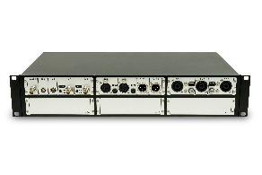
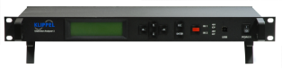
KLIPPEL Analyzer 3 (alternatively Distortion Analyzer 2) is the hardware platform for the measurement modules performing the signal generation, data acquisition and digital signal processing in real time.

For more information check specifications: H1, H3

LPM – Module

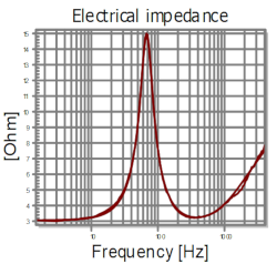
Module to identify the electrical and mechanical parameters of electro-dynamical transducers by measuring the voltage and current at the transducer terminals.

For more information check specifications: S2

TRF

The Transfer Function Module (TRF) measures the transfer behavior of a loudspeaker transducer, along with distortion analysis.

For more information check specifications: S7

Scanning Vibrometer Hardware (SCN)

The Scanning Vibrometer (SCN – “Klippel Scanning System”) performs a non-contact measurement of the mechanical vibration and geometry of cones, diaphragms, panels and enclosures.

For more information check specifications: C5

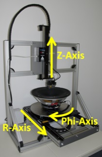
Alternative ways to gather SCN/LPM data

Poly2SCN Module

Module for importing surface vibration data to Klippel SCN format.

For more information check specifications: S45

Hardware setup

RMA does not require hardware setup of its own since its analyses are purely postprocessing of input data which is gathered using other measurement modules (see table above). All hardware-related setup information is covered in the respective manuals of the modules concerned with measurement data acquisition.

RMA Tutorials

Tutorial Overview

These tutorials give step-by-step instruction how to use the Rocking Mode Analysis module (RMA).

• Tutorial 1 – Viewing the results – offers a quick overview of the analysis. It introduces the way the results are presented in RMA after the operation is executed. It is especially useful for new users of RMA.

• Tutorial 2 – Generating RMA results step by step. This tutorial is more in-depth. It describes all steps necessary to determine valid results with RMA. This guides the user though the entire process from scratch, including the measurement.

• Tutorial 3 - Understanding interaction of imbalances - shall offer guidance how the contributions of mass, stiffness and Bl imbalances interact with each other. This allows the user to understand why the results look like they do.

Tutorial 1 – Viewing the results

Open the Example database

Example data used in this manual is stored in the Web Example database. If not downloaded already, get it from the latest R&D release <https://www.klippel.de/go/current-rnd-release> and open the web-based database.

See also

View Results for general information on how to download this database, open and view results in dB-Lab.

Navigate to section “Scanning Laser Vibrometer (SCN, RMA, HMA)””. In the folder “Rocking Mode Analysis (RMA)” select the object “RMA Microspeaker”.

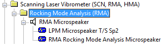
The RMA requires Thiele-Small parameters, which can be conveniently provided through a link with a Klippel RMA operation (users of the Poly2SCN module are also given the option to provide these parameters via manual or clipboard input). Along with that, RMA requires distributed vibration data in Klippel SCN format. The tutorial example SCN data is included in the operation “SCN Data Container RMA Microspeaker”.

Open the operation RMA and review the window Summary

Severity of the rocking problem

The severity of the rocking problem is described by the Relative Rocking Levels RRL, which is the dB difference between the kinetic energy contained in the piston mode (AAL₀) and the energy contained in the rocking mode (AAL₁ or AAL₂). Note that a stable driver in terms of rocking modes accumulates only small quantities of rocking energy and consequently displays a large negative RRL value. As a rule of thumb, drivers showing an RRL below –20dB are usually not critical from a rocking point of view. Drivers with RRL values above that threshold shall be examined more carefully. The higher the RRL, the more pronounced is the rocking motion. In rare cases, drivers can even reach a positive value of the total RRL_T, indicating a very severe rocking problem. In physical terms such result indicates that the mechanical energy associated to the rocking mode at its resonance frequency is larger than for the piston mode at that frequency. Our tutorial example microspeaker transducer shows an RRL of -8.5 dB, which indicates that the rocking is pronounced.

Note

Even a strong rocking resonance might not be clearly visible as a peak in the passband-region of the frequency response. In one-point measurements of vibration displacement/velocity with a laser in the center of the diaphragm, you will measure very close to the crossing-point of the nodal lines of both rocking modes. In acoustical measurements the mode will also be hard to detect due to its very low sound radiation (“quadrature component”).

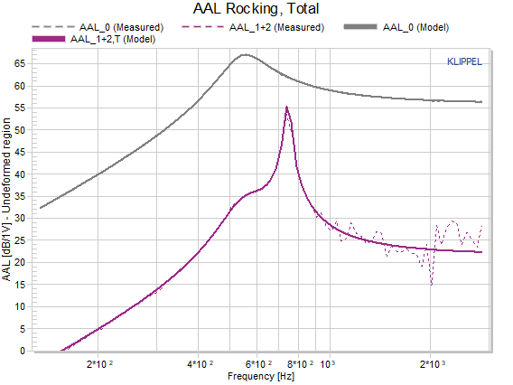
At this point, take a quick side-look at the result window AAL Rocking Mode n which shows similar information to above table, in a visual format: the AAL vibration energy summed up for both rocking modes in comparison to the piston mode. The relative position of the rocking modes in frequency and level relative to the passband and fundamental resonance become directly obvious. The window also provides you a first idea of how well the fitting of the rocking-mode model (purple line) fits with the measurement data (purple dotted line). This can serve as a first indication for how well the overall result can be trusted. More detailed diagnostic information is given in the result window Errors / Warnings. More details about quality assessment of the diagnostic result are given in section Checking the results.

Rocking excitation: Combined Force Ratio

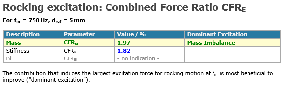
Return to the result window Summary to evaluate the excitation of rocking modes, which is described by the Combined Force Ratio CFR_E (index E = Excitation: Mass, stiffness or motor strength Bl). This value summarizes the magnitude of the excitation forces induced by the root causes, combining both rocking modes. It informs us about which physical parameter (mass, stiffness or Bl) causes the strongest excitation of rocking modes. The CFR is the ratio between the asymmetrical forces producing imbalances and the symmetrical force F = Bl*I acting on the coil.

Note

Cross-modal coupling of the two rocking modes is neglected in the calculation of the CFR, which means that the modes are treated as if they were independent of each other. More details about this are found in the RMA-Reference.

This result is calculated at the geometrical average resonance frequency of both rocking modes. The larger the CFR is, the more excited is the rocking mode. In the example above, there is no indication of Bl asymmetry so that this parameter is excluded from further analysis. Instead, this driver presents a mass imbalance induced excitation force with magnitude 1.97% of the piston mode excitation force. Since it is the largest contribution, it is labelled “dominant” here. Anyhow the imbalance of stiffness induces an excitation force in the same range of magnitude (1.82%) so that both shall be looked at in more detail for improvement of the transducer. Here we shall especially consider the phase relationship for the forces caused by the mass and stiffness imbalances, which will be discussed in detail in Tutorial 3 - Understanding interaction of imbalances.

Root causes: Imbalances

Once the dominant source(s) of excitation is/are identified from the evaluation of forces, we shall investigate the root causes that induced these forces: The Imbalances (=inhomogeneities) in the distributions of mass, stiffness and Bl force factor. The last section of the “Summary” window shows how far the centers of mass, stiffness (and eventually even force factor) are offset from the geometrical center and in which direction.

Hint

Keep a record of the orientation of the driver during the scanner measurement, since the RMA direction angles are referred to the angles of the driver on the turn table.

This information is visually depicted in the imbalance diagram which gives a very valuable indication of where the physical root cause (design-inhomogeneity or manufacturing imperfection) is located on the examined DUT.

Note

The offset values for the center of imbalance from the diaphragm center are approximate values. The reason for this is that they are scaled by the rotational stiffness of the diaphragm (i. e. the rotational “spring-stiffness” that counteracts tilting in the main directions of rocking motion). The latter can though only be roughly approximated by RMA. More on that can be found in the end of the chapter on Imbalances. Anyhow, the indicated direction where the imbalance centers are located are less affected by this.

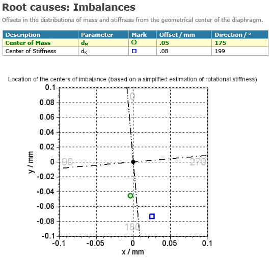
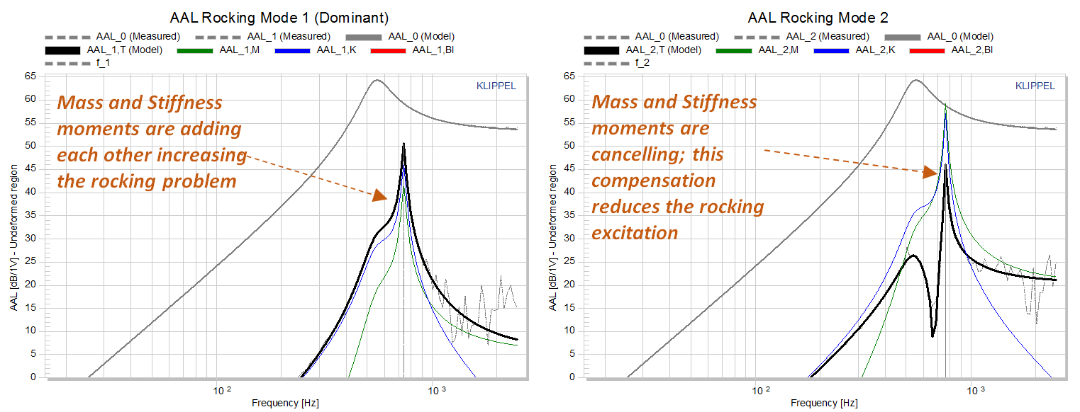
The situation above is an especially interesting case. Here mass and stiffness imbalances compensate each other to large extents along the direction of mode 2 (double-dotted line) due to their opposite phase, whereas they add up in the direction of mode 1 (single-dotted line). If this is not directly intuitive to you, check the AAL Rocking Mode n or the Relative Rocking Levels RRL. For mode 1 the total AAL is larger than the contribution of mass and stiffness imbalances alone and for mode two it is the other way round. A thorough walk through of the interpretation of mode interaction is found in the RMA reference in the chapter about Modal Force Ratio MFR or in Tutorial 3 - Understanding interaction of imbalances.

Open the windows “Rocking Mode 1” and “Rocking Mode 2”

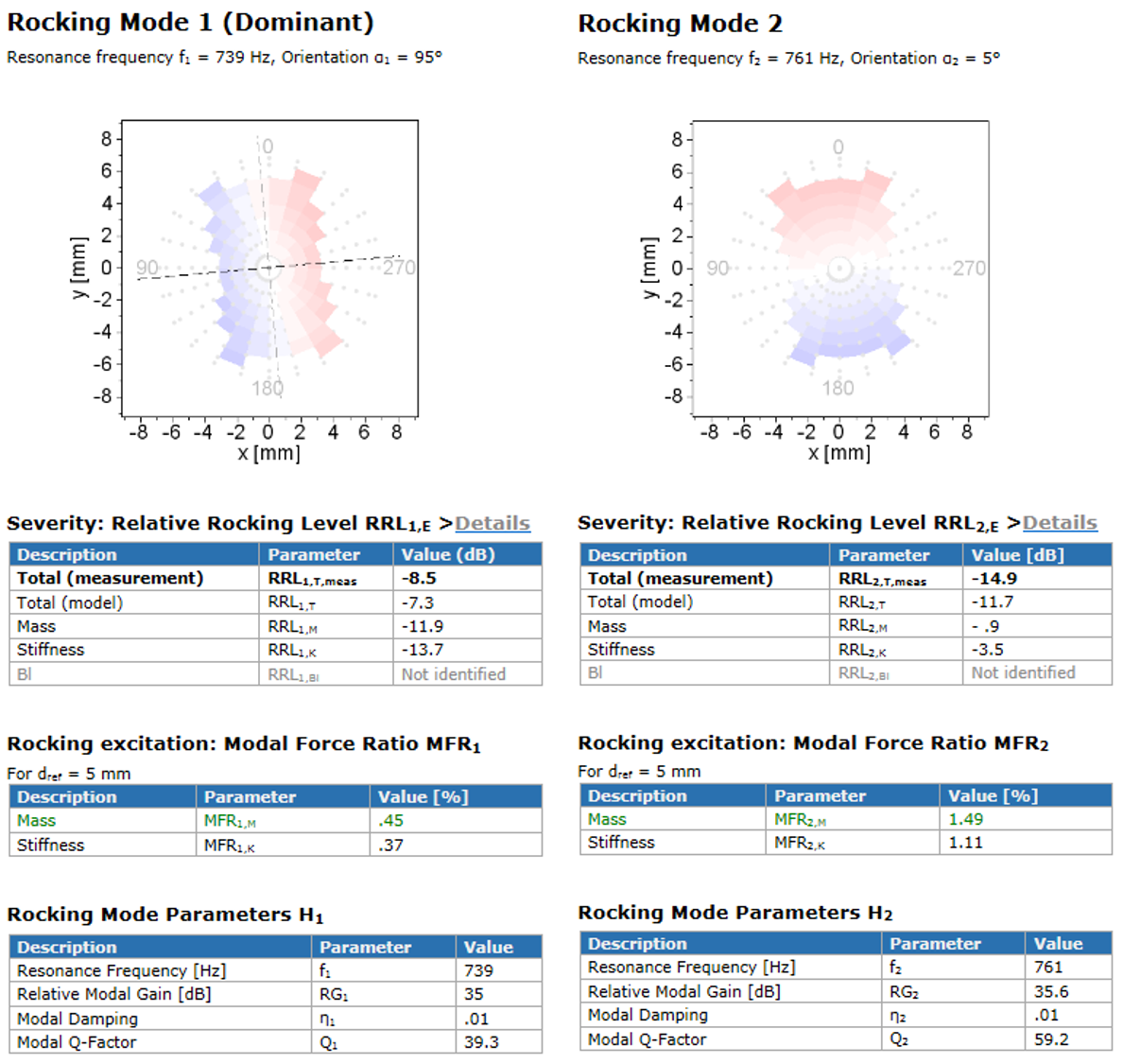
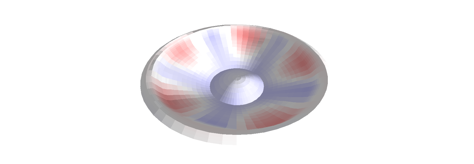
These windows provide details about the two rocking modes individually, including the decomposition into the contribution of different root causes, along with the mode shapes of two rocking modes as color maps. The mode with stronger excitation is labelled with the suffix “dominant”. Since the mode-shapes present their displacement maximum at an angle of 90 degrees relative to each other (>modal orthogonality), the dominant mode is often significantly stronger than mode two. The modal resonance frequencies f₁ and f₂ and angular orientation of the modal maximum are shown in the upper part of the windows. In addition, the direction of maximum modal amplitude is highlighted with a thick black dotted line called α1 and the rotational axis is depicted by a thin grey dotted line. To understand the values given for the Relative Rocking Levels decomposed per root-cause, compare the result-window AAL Rocking Mode n, which is introduced in greater detail in section Checking the results. The Modal Force Ratio MFR table shows the contribution of each root cause in excitation of the modes, relative to the excitation force of the piston mode. The result is presented in percent.

Finally, the Modal Parameter Tables H₁ and H₂ show the modal parameters required to explain the transfer from these asymmetrical forces to the produced output tilting, including the Relative Modal Gain RG, the Modal damping η and the Modal Q-factor Q.

Note

The usually very high Q-factors of rocking modes that explain why relatively small forces in the dimension of few percent of the total voice-coil force are enough to excite these modes to high amplitudes. The reason for this low damping is that the air is only pumped from side to side in the cavity below the membrane during rocking, with no airflow through the narrow magnetic gap, where friction losses would occur otherwise.

Tutorial 2 – Generating RMA results step by step

Measuring LPM and SCN input data for RMA

The SCN measurement data of the microspeaker used in this tutorial is provided in the dB-Lab web example database. If not downloaded already, get it from the latest R&D release <https://www.klippel.de/go/current-rnd-release> and open the web-based database.

See also

View Results for general information on how to download this database, open and view results in dB-Lab.

Navigate to Scanning Laser Vibrometer (SCN, RMA, HMA)Rocking Mode Analysis (RMA)RMA Microspeaker.

In the following, the steps of the scanner setup are described precisely in order to be applied to other drivers.

Step 1: Power on

Power on your measurement hardware including amplifier.

Hint

Before starting the measurement, give the laser some minutes to heat up.

Step 2: Treat the diaphragm-surface

Treat the diaphragm=surface of your transducer so that it is

• Opaque (= non-transparent)

• Bright (= white)

• Matte (= reflecting diffusely)

• free from artifacts like loose particles, fibers or dust.

Note

Detailed information:

1. Ensure a dust-free surface of the diaphragm.

2. Carefully spray or rub the surface with a thin layer of matte white powder.

3. In case that fibers start sticking up, rub the diaphragm carefully and repeat above treatment.

Observe:

For microspeakers and headphones, be very careful not to bias your diaphragm with too much coating. Spray it thin, but still opaque!

Step 3: Start the Klippel SCN software

Start the Klippel SCN software and initiate a new scanning process. Choose menu option “file>perform new scan”. If prompted, choose your desired hardware and follow the instructions for the hardware calibration of the laser axis.

Step 4: Place the transducer in the center of the turntable

After completed laser-calibration, when advised by the software, place the transducer in the center of the turntable, either directly on the plate or on another dedicated support (e. g. Klippel Microspeaker Stand)

Check this:

• Before placing the transducer, make sure that the scanner is at start position for the phi and r axle. [1]

• Assure that the rear side of the transducer diaphragm is vented in the same way as supposed to be in the final application.

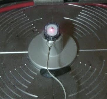
• The diaphragm should be in parallel to the turntable surface, as it can be seen in the picture. [2]

[1]

By default, the turntable shall be centered directly after laser calibration and after a completed scan. In case of doubt you can use the software tool “direct motor control” (press F5 in the scanner software or use the menu “tools”) and click on the house-symbol (“home”).

[2]

The orientation of the transducer on the turntable since it is the reference for all angular information presented by the RMA module. It is good practice to decide on a convention for this that you follow every time. One good option is to always align the electric terminals of the DUT with the direction labelled 180° on the SCN turntable.

Caution

Clamping the transducer can have major influence on the results. Apply only very small forces to the rim of headphone drivers during clamping. Deforming the transducer only slightly will change the strain in the diaphragm which may alter your rocking behavior a lot.

Step 5: Perform an LPM (linear parameter measurement)

Before proceeding with the scan setup – if you have not already done this - perform an LPM (linear parameter measurement), without repositioning the loudspeaker transducer on the turntable.

• Pressing “F4” in the SCN software will launch dB-Lab for you

• If you do not have a database open already, open one or create a new one. Create a new object (> loudspeaker symbol) and choose the template “RMA Rocking Mode Analysis”.

• Edit the properties of the operation “LPM for RMA” (press Alt+Return):

• Frequency: F_max = 10kHz

• Data reduction: 30 points/octave

• Connect your transducer to the highly current-sensitive channel of your KA3 or DA2. Adjust settings of input channel accordingly. [3]

• Go through the following checklist and then run the operation.

• Refine your settings until you reach good quality data. Refer to the LPM documentation if needed.

[3]

For DA2 you do this by physically switching the cable to the respective channel (SP 1: Low sensitivity, SP 2: High sensitivity)

Hint

If the system does not allow you such settings, reduce the amount of datapoints per octave. Anyhow, do not go below 20 points per octave. More points will give better fitting. For the same reason, keep the low frequency limit of the measurement as low as possible.

Note

Checklist for LPM Measurement

The LPM measurement (which provides T/S parameters of the DUT that are required by RMA) can be done either directly before starting the scanner process or directly after finishing it. RMA will read that data directly from the LPM operation which is selected in the RMA property page. (See next chapter)

• Make sure that the scanner is at start position for the phi and r axle. [4]

• Make sure that the loudspeaker transducer is positioned in such a way that the measurement is taken precisely at its center.

• Ensure that this centerpoint of the LPM coincides with the center of the SCN grid that you have defined. This improves the accuracy of the RMA. The ideal result can be obtained if the driver is not moved between the LPM and SCN measurements.

• Before starting your measurement, check the status LED of the laser to ensure that it is operated within its ideal working range. Use manual motor control otherwise.

• Depending on the piston resonance frequency f_s of your driver, the LPM might display a message asking to reduce your maximum frequency F_max in order to improve impedance fitting. Since you need LPM data in the complete frequency span of your SCN, this message can be disregarded.

[4]

By default, the turntable shall be centered directly after laser calibration and after a completed scan. In case of doubt you can use the software tool “direct motor control” (press F5 in the scanner software or use the menu “tools”) and click on the house-symbol (“home”).

Step 6: Read the maximum displacement

Read the maximum displacement that occurred during your LPM measurement, X_LPM,max

• Open your LPM Operation

• Open the result window “x(t)”

• Read the maximum value using the cross-cursor (which can be activated by keyboard shortcut “Q”).

Step 7: Connect transducer to low sensitivity channel

Make sure the transducer is connected to KA3/DA2 low sensitivity channel. For KA3 it can be either done by switching the cable physically like on DA2 or through changing software-routing in dBLab menu Hardware ‣ KA3 ‣ Signal Configuration (Ctrl + Shift + L).

Step 8: Set signal characteristics

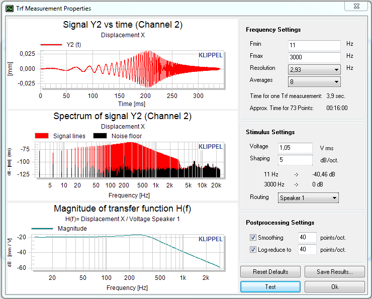
Return to the Klippel SCN software. In the Scanning wizard tab “Setup”, click on “Edit TRF setup” to set signal characteristics. Use your previous knowledge about the driver to check frequency-range.

Frequency Settings

• F_min [5] = 11 Hz (F_min<=f_s/4)

• F_max [6] = 6 KHz (F_max ~= 4*f _rocking,max)

• Resolution [7] = 2.93 Hz

• Averages [8] = 4

[5]

To accurately model the piston mode and distinguish between the root causes for rocking, the frequency range needs to include enough points below the piston resonance frequency f_s of the DUT. F_min should be less than two octaves below f_s.

[6]

For transducers with exceptionally high-frequent rocking mode frequencies, an upper frequency limit of 8 kHz can be appropriate.

[7]

In some rare cases of rocking modes lying very low in frequency, 1.46 Hz can improve fitting.

[8]

In cases of drivers being protected by screens or in vacuum, where the optimal optical access of the laser to the surface is limited, or if S/N ratio is generally low, a larger number of averages improves the signal quality substantially. This setting will prolong scanning time.

Caution

Always check voltage if you change F_max!

The choice of F_max frequency greatly affects the voltage-distribution of your stimulus. Reducing F_max increases the applied voltage at f_s, which could damage your speaker. If F_max is changed, always reset voltage to <1V.

Stimulus Settings

• Shaping: 5 dB/oct (important!)

• Voltage (max): The stated voltage is valid at F_max and shaped relative to that value at other frequencies.

Postprocessing settings

• Activate both smoothing and log reduce

• You should use as many points as possible, but still keep log reduce on

• 40 points/octave are recommended for KA3 (If you are using DA2 you might have to reduce this number)

Hint

How to find a suitable excitation voltage

• It is an iterative process

• Make sure you understand all (!) restrictions below, before (!) applying voltage to your transducer

The stated voltage is applied at F_max. “Shaping” reduces the voltage towards lower frequencies. The largest displacement amplitude appears around piston resonance frequency f_s. You should drive your speaker in the linear range.

1. Make sure that Fmax is several octaves above fs, so that shaping can limit displacement.

2. Ensure that shaping is set to 5 dB/oct. Shaping will help to protect your speaker and at the same time secure a good the S/N ratio.

3. Only after shaping is enabled, start with low voltages (around 1 V) - ensure that you are scanning the centerpoint and perform a test run.

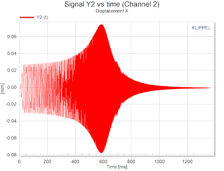
4. Check maximum displacement amplitude in your time-signal (you can read it from the diagram “Signal Y2 vs time” at the top of the window). Compare it to X_LPM,max, the maximum displacement of your previous LPM voltage slowly and gradually and aim for a similar centerpoint-displacement as X_LPM,max. Do not go beyond X_LPM,max*2.

Caution

Too high voltage applied to your speaker can harm your hearing (and DUT).

Step 9: Check signal-to-noise-ratio

Check signal-to-noise-ratio for your TRF measurement properties. Make sure you have connected your loudspeaker transducer to the channel of your measurement hardware with low current-sensitivity.

Hint

How to handle signal-to-noise-ratio

• Using the button “Test” in the TRF Measure­ment proper­ties to perform Test-TRFs on different regions on the diaphragm.

• Pick some points using the motor control (close to the surround, main part of the membrane, steeply inclined part of dust-cap, diaphragm center) and check that S/N ratio is better than 8 dB in the frequency ranges of measurement.

Otherwise, try the following:

• Increase number of averaging steps. This will improve S/N but also increase scan time.

• Carefully adjust your stimulus voltage. Avoid creating excessive distortion.

• Check that your scanned frequency range is well adapted to the needs of RMA. Note that you have to repeat the process of finding a good excitation voltage in case you change F_max.

• Consider improving surface treatment of your membrane according to step 2 above.

• If you regularly run into problems with S/N check that your laser model is well suited for the task. You will find more information about laser models in your Klippel Hardware Manual.

Step 10: Choose Scanning method

Choose Scanning method Vibration and geometry

Select the scanning mode:

• For regular cone-shaped transducers “normal scan” will in most cases be the appropriate scanning mode.

• For micro­speakers and headphones “flat scan” can be a better choice. In doubt, refer to scanner documentation.

Step 11: Define your SCN grid

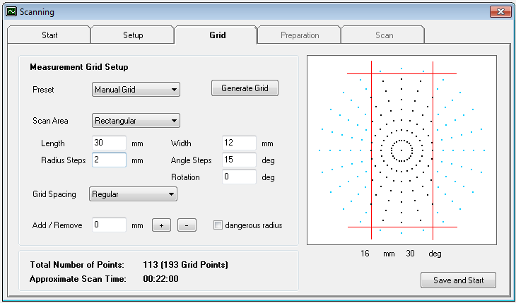
Use the “manual grid” preset to define an appropriate and sparse grid for your driver. First choose the general shape of your driver (rectangular or circular) under “Scan Area”. Then define the scanning grid as follows:

• 6 rows of points between the center of the transducer and the middle of the surround.

• Angle steps 45 degrees

• Remove measurement points in areas of the membrane where the results are not expected to be reliable. (e. g. at very steep inclination angles of the dustcap or at joining lines of several parts)

• You can use both regular grid-spacing or setting “sparse”. Using the former is somewhat more exact, using the latter is faster, especially for microspeakers.

Some motivation for the settings

Rocking mode analysis does usually not require a dense scanner grid. Usually only the suspension parts or the outer parts of the diaphragm are deformed under the forces and moments acting in the frequency ranges around the rocking resonances. A measurement focused on the majority of the center part of the diaphragm that is moving as a rigid piston will provide accurate RMA results.

• A larger number of scan points will improve the signal to noise ratio of the preprocess stage of the RMA.

• All the results provided by the RMA are referred to the coordinate system of the turntable.

• The absolute minimum requirement is to use 3 radial lines in the rigidly oscillating part of the diaphragm (non-deformed area = surround completely excluded). If you choose to include the surround in the scan, use more radiusses.

• You can then detect the actual rigidly oscillating area as described in step 16 below.

• Exceeding the minimum requirement for spatial resolution will improve fitting accuracy.

Hint

How to measure the dimenions with motor control

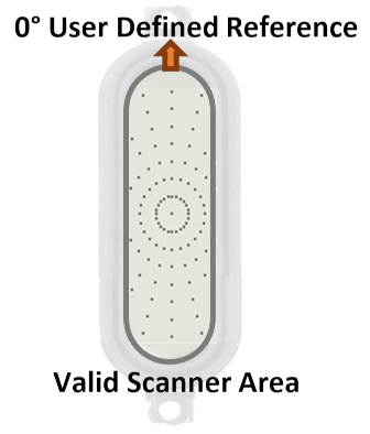
You can measure the dimensions of your transducer using the direct motor control (that can be launched from the “tools” menu of the SCN software or by pressing “F5”). Move the laser beam across your driver using the software buttons and read the coordinates at the bottom of the control window.

Step 12: Start the scanning

Start the scanning process and follow the further instructions by the SCN software.

Hint

Repeat LPM after the Scanning Process

After the scan, we recommend to run another LPM and compare the results. A good practice to make sure that your transducer is fine and your results can be trusted. This step is optional.

Searching for rocking mode problems with the SCN software

The following steps of the tutorial can be done by visualizing the content of SCN Data Container RMA Microspeaker which is found in your dB-Lab Web Example Database. Navigate to Scanning Laser Vibrometer (SCN, RMA, HMA)Rocking Mode Analysis (RMA)RMA Microspeaker. Open the property page and click on Visualize SCN data. After opening it (an SCN license is required), follow the instructions below.

Step 13: Show data “on axis”

Make sure you are showing data “on axis”

• Switch over to tab “radiation analysis”

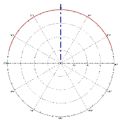
• In the left diagram showing the polar plot, make sure that the directional cursor is set to on-axis-position (0°) [blue dotted line pointing straight up – drag with your mouse to move it if needed.]

• Switch back to tab “animation”.

Step 14: Investigate peaks in the Quadrature Component of AAL

After finishing the scanner measurement, select the SPL decomposition option as follows:

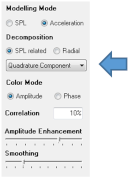
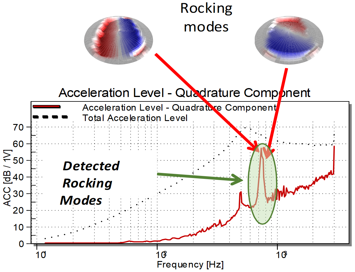
• In the Acceleration Level plot of the quadrature component, look for resonance peaks having AAL level close to the total acceleration level.

• For any suspicious peak, use the animation to check whether the mode-shape corresponds to rocking motion.

• Note down the rocking frequencies that you have identified. You will need these later to determine the correct analysis frequency range in step 21.

Note

Peaks in the quadrature component are the first indicator of the existence of a substantial rocking mode.

These peaks provide information about the magnitude of the rocking problem, but not the root causes. Very often, you will also see only one peak for two rocking modes (which usually lie close together in frequency) and hence not be able to separate them. In all of these cases the RMA module will offer you valuable additional analytics.

Assessing valid geometrical dimensions

Measure the dimensions of the rigid­ly oscillating part of your diaphragm at rocking frequency. The values that we determine here are required as an input parameter to the RMA.

Step 15: For drivers with round geometry

• Determine rigidly moving radius r_rigid.

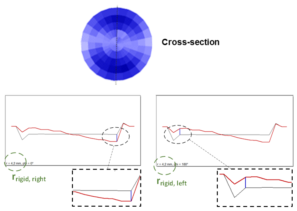
• Switch to tab Radiation Analysis and orient the black dotted line in the direction of the maximal rocking amplitude (where the blue color has maximum intensity).

• Switch to tab Cross-section view and animate the motion. Pause the animation at maximum displacement.

• Locate the outer end of the rigidly oscillating area of your diaphragm. You will see a distinct change of angle there. Click on that point to set a cursor (a blue line appears). Read the radius value in the lower left corner of the animation window.

• Animate the structure again and freeze it in the other position of maximum displacement. Read the respective maximum undeformed radius on the other side of the membrane, again using the cursor.

• If the radius readings on both sides deviate, note down the smaller one.

• Specify r_rigid in the RMA parameter input page (step 20)

Hint

Go to tab Animation in your SCN software to set the cursor at rocking-frequency of the quadrature AAL (as described in steps 14 and 15 above). Animate to verify the rocking motion.

Step 16: For rectangular drivers

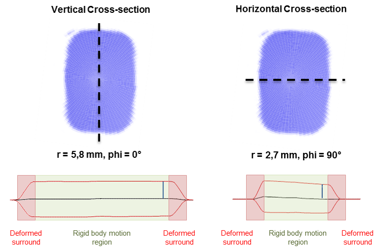
• Determine rigidly oscillating half-length and half-width [9]

• This case applies to our tutorial example.

• Similar to what is described above for round drivers, find the orientation of maximum displacement in the tab Radiation Analysis.

• Go to the tab Cross-section view. In the left inferior part of the animation window, read the radius value that is inside the rigid body motion region as shown in the figure. Repeat the same process for the phi angle = 90° (Horizontal). Note down the determined values for half-length and half-width.

• r_rigid=min(r_rigid,left, r_rigid,right).

• Specify 0.9*r_rigid in the RMA parameter input page (step 20)

[9]

Motivation: To remove noise, we are fitting the model of an oscillating plate to the rigidly tilting part of the diaphragm. All analysis of root causes will be done on this fitted plate model. For the plate fitting it is necessary to identify the main axis of oscillation. If a small error is done in the identification of the angle of the main axis of the vibration mode, then this slightly misrotated plate can - if its size is very close to the actual rigid area of the diaphragm - overlap with the surround for dynamic rocking mode model and the measured LPM. One consequence of this can be large errors in the identification of the root causes (amplitude and direction). The rule of thumb to use 90% of the measured dimensions as input to RMA will remove this risk and keep you on the safe side while staying close to the true rigid dimensions of your DUT.

Caution

For rectangular drivers, you should reduce r_rigid to 90% of its measured value before specifying it in the RMA input page. Using the complete measured “rigid diaphragm” could cause problems.

Make sure that the selected limits (radius, length, and width) do not include the surround, because it will cause a mismatch between the dynamic rocking mode model and the measured LPM!

Step 17: Remove artifact points in the scan

Check the animation of the scanner data for points with unreasonable response: Peaks, dips, dead points.

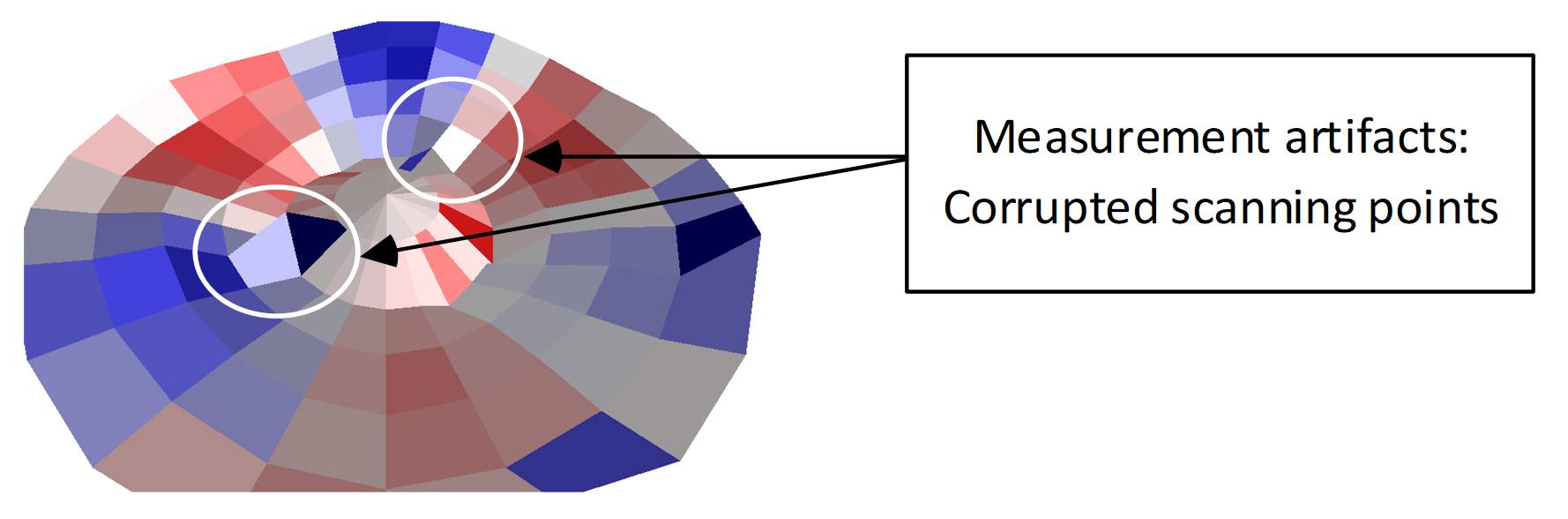
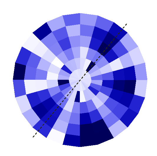
Switch to tab “radiation analysis” and orient the dotted line by dragging it with the left mouse-button pressed down so that it intersects the corrupted point.

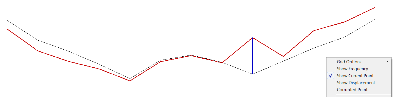
Switch over to cross-section view mark the corrupted point with a mouseclick. Open the context-menu by right-clicking and select “corrupted point”. Continue this process until all corrupted points have been treated.

Step 18: Export the SCN data

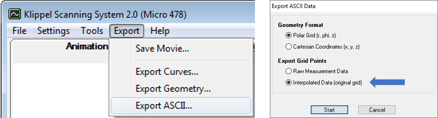
Export → Export ASCII… and select “Polar Grid (r,phi,z)” for the “Geometry Format” and “Interpolated Data (original grid)” for the “Exported Grid Points” options. This ensures that no grid points without data will occur. This will generate a file of type .sce containing all geometry and vibration data. Feed this to RMA.

Note

There are two kinds of .sce files. Those with very small size (<0.1 MB) do not contain the complete dataset and only a link to raw data. RMA cannot read these. Use the export function as described above.

Setting up the RMA operation

The aim of this section is to explain how to set up the RMA Module in a step-by-step instruction. We will follow our microspeaker example from the previous sections.

Step 19: Start dB-Lab

Open up the dB-Lab Web Example Database and navigate to the object Scanning Laser Vibrometer (SCN, RMA, HMA)Rocking Mode Analysis (RMA)RMA Microspeaker.

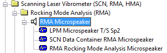
The web example database contains the RMA operation and the LPM Microspeaker T/S.

Step 20: Open the property page of the RMA operation

• Open the property page of the RMA operation -> Input

• Mark the RMA operation in dB-Lab and right-click on it to select “properties” (Shortcut: Press Alt+Return)

• All the input parameters required for running the operation are explained in the following three steps.

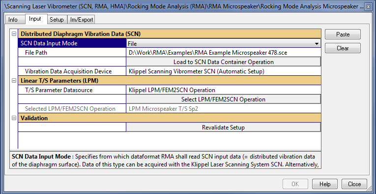
Step 21: SCN and T/S input data

RMA requires vibration data in Klippel SCN format and T/S parameters, which preferably are provided through a linked Klippel LPM operation of the DUT.

Step 22: Specify SCN file and LPM operation

Navigate to input property page tab “Input”.

Distributed Diaphragm Vibration Data (SCN): The *sce file that has been cleaned from measurement artefacts and exported from the SCN interface (step 17/18) should be loaded. There are two ways to provide SCN data to RMA. You can either:

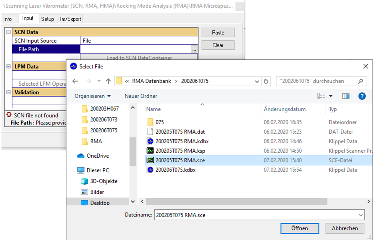
1. Read from an .sce file on your hard disc. Choose option “SCN Input Source ‣ File” in this case and specify the path to your file in the field “File Path”. This will automatically load your data. We recommend to transfer your file into an SCN Data- container (which is optional). To do this, select “Load to SCN datacontainer”.

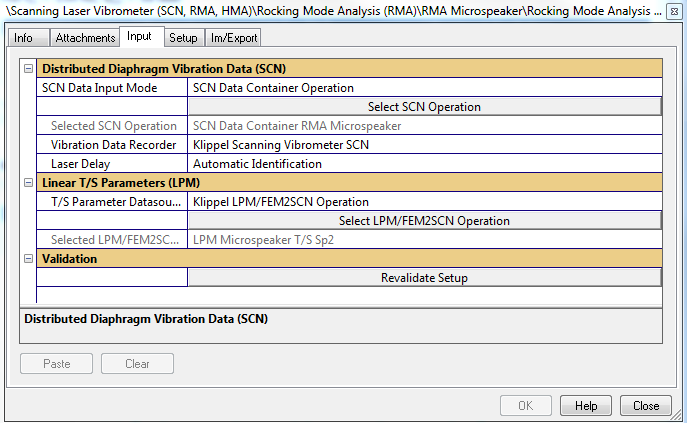
2. (Preferred) From an SCN data container. This makes your data follow along conveniently with your dB-Lab database. Choose option “SCN Data Input Mode ‣ Data Container”. The fastest way to transfer SCN data into a data container is described under option 1 above. You can also create an SCN datacontainer operation manually and load in the data there. Afterwards, link the respective SCN operation to RMA using the button “Select SCN Operation”.

To follow the tutorial example, choose the SCN file provided in “SCN Data Container RMA Microspeaker”

Laser Delay: For accurate modelling of phase, RMA needs information about the delay of the scanning laser signal relative to the voltage measurement. This value can be either determined automatically by RMA or you can specify a known laser delay manually.

LPM Operation: Choose the related LPM measurement containing the linear parameters of your driver. The RMA finds only LPM operations that are placed under the same object (>loudspeaker symbol). To copy the operation there, use CTRL+C and CTRL+V. Afterwards, use the button “Select LPM operation” to specify, which LPM operation shall be used in RMA analysis.

In this tutorial, the operation “LPM Microspeaker T/S Sp2” is chosen.

SCN data from HDD file

SCN Data from Datacontainer

If you have access to a license for the dB-Lab module Poly2SCN, you are given access to choose the option “Other” in the field “Vibration Data Acquisition”. This unlocks the option to specify the amplifier gain in your signal chain, which is useful for measurement devices that do not measure the actual excitation voltage at the loudspeaker transducer terminals. RMA offers an option for automatic amp gain identification, which provides optimal fit of the vibration data with the provided linear T/S input parameters.

The automatic setting will work well in the large majority of cases. Anyhow exact automatic estimation of laser delay is tricky at the relatively low frequencies where RMA operates. It is therefore a good idea to inspect the result of the laser delay estimation (which can be found in result window “Errors/Warnings”) in cases when the “LPM fitting error” is high or when the phase fitting looks unreasonable. Comparing with other RMA operations with good fitting will allow you to extract the laser delay value of your setup, which is very constant. In such cases you can provide this value manually to improve the RMA result.

Several LPM measurements can be done in the object and later the best can be chosen from the list.

Please note: Loading of LPM and SCN data is triggered once, directly after the respective operations have been selected. If data inside these source operations is changed afterwards, RMA will not automatically notice this. Use the button “Revalidate Setup” to trigger a fresh load-in of LPM and SCN source data. This will also update the dependent data (allowable frequency ranges and geometry) that is used in the data consistency checks in the other tabs of the RMA properties. A reloading of data is always triggered automatically once the RMA operation is executed (>green arrow button)

If you have access to a license for the dB-Lab module Poly2SCN, you can also specify Thiele-Small parameters manually or copy it in using our clipboard import.

Step 23: Specify diaphragm geometry

Usually not the entire scanned geometry is used. RMA fits a rigidly oscillating plate to the vibration data. For this, you must make sure to include only the part of the diaphragm into the analysis, that vibrates rigidly (=without deformation).

Step 24: Specify rigidly oscillating geometry

Switch to input property page tab “Setup” Choose the geometry of your DUT > rectangular or circular.

Specify 90% ofthe rigidly oscillating dimensions of the driver. You will need the value for r_rigid that has been gathered in tutorial step Assessing valid geometrical dimensions.

For rectangular drivers specify 90% of the rigidly oscillating length and width to avoid problems with slightly rotated geometries.

The settings stated below apply to our tutorial example and to other rectangular drivers.

• Geometry: Select Rectangular and type the following values:

• Length: 5mm (=0.9*distance from the center of the driver to the end of the rigidly oscillating diaphragm length in [mm])

• Width: 2.9mm (=0.9*distance from the center of the driver to the end of the rigidly oscillating diaphragm width in [mm])

Step 25: Processing frequency settings

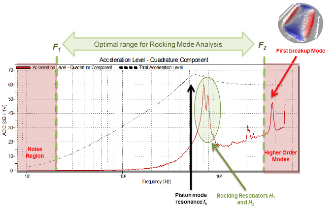
The rocking mode analysis is valid only at frequencies below the first breakup mode of the transducer diaphragm (here the central part of the diaphragm shows major deformation, i. e. the model that assumes a rigid diaphragm will become inexact. Also, we shall not include major noise components, which might be present at the lower end of the measurement frequency scale. For this reason, the frequency range of analysis where these conditions are fulfilled has to be selected by the user. An incorrectly chosen frequency range will reflect in the Spatial SCN plate-fitting error.

Step 26: Specify processing settings

Frequency Limits

The frequency limits [f_min f_max] can be read in the scanner visualization software based on the following criteria:

• Low frequency limit fmin: MUST be always at least one octave below the fundamental resonance frequency (f_s) of the transducer. Recommended: two octaves below. RMA requires low frequency information to differen­tiate between mass and stiffness excitations. Anyhow it should not include high noise level. Recommendation: f_s/4 < f1 < f_s/2

• High frequency limit fmax: MUST be at least 1 octave larger than the most highfrequent rocking resonator peak, BUT has to be less than the first breakup mode. Recommendation: max(f_rocking[1,2])*3 < f2 < 0.9* f_breakupmode1

Exclude Frequency Range

Exclude Frequency Range in Category “Advanced”. [10] You can exclude a certain frequency band that is contained inside the analysis range specified above using this advanced option. This is not necessary in 99% of the cases.

[10]

This option allows exclusion of effects that corrupt data validity in only a small frequency range (breakup-modes, noise artifacts). To avoid that the RMA algorithm confuses parasitic resonance peaks (like structural resonances such from spider, mounting case, etc) with the rocking resonance of the diaphragm. Exclude the respective frequency range from identification by specifying lower and upper limit frequencies. Use this with care since excluding higher order modes this way can affect the phase behaviour that RMA uses to determine the direction of the centers of imbalance. It is preferred to only restrict the frequency range without this option.

Note

Usually the quadrature component of the SPL related decomposition in the scanner software reveals the existence of a substantial rocking mode problem.

Computation speed

This parameter is related to the time required for the RMA to perform the complete analysis. With setting “slow”, the calculation will use the full number of frequency points and geometrical scanned points available in the scanner measurement. A selection of “normal” or “fast” will decrease the number of frequencies used in the identification according to the selection and pick a suitable set of geometrical measurement points if the selected mesh contains more than 140 points.

Note

Selection of faster speeds will reduce the computational time but some considerations need to be taken into account.

1. For rocking resonators exhibiting high Q-factors (undamped systems, Q larger than 20), it is recommended to use setting “slow”, because such peaks require a larger number of frequency points to be accurately Identified.

2. In cases where the rocking resonators are more damped, the computation speed can be set to “normal” or “fast”.

For the example in this tutorial the setting “normal” is sufficient, despite the large Q-factors. The user can run the operation using slow or fast and see the differences.

Starting the operation

Step 27: Run the operation

Once the RMA setup is done and the input parameters introduced, please run the operation by clicking the green arrow button.

The RMA will load the measured data and will perform the required preprocessing and data conditioning to be used in the identification stage.

Checking the results

When the RMA is finished and the operation symbol turned blue, double-click on the operation to see the results. The window will look something like this:

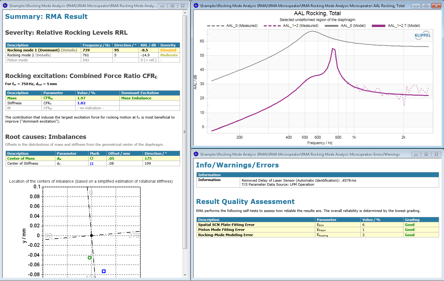
The displayed results present an overview of the most important information for the rocking mode diagnostics of this microspeaker.

Step 28: Check the quality of the fitted system

Check the quality using the result window Errors/Warnings

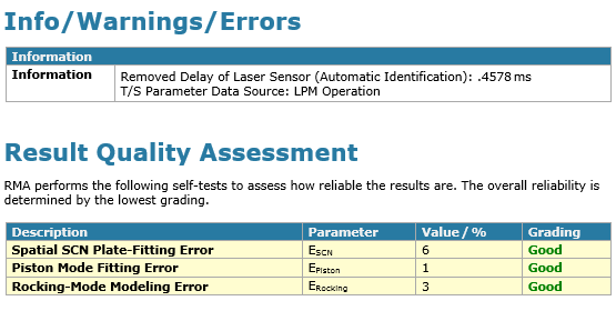
This window provides a summary of the fitting quality in three sections. All of these error measures depend highly on the dimensions provided by the user (the chosen frequency range, the quality of the LPM, and the scanner measurements). More information about the definition of the errors and how to improve the result can be found under Errors / Warnings in the RMA Reference.

Also have a quick look in the SCN software to verify that RMA has correctly identified the rocking resonators seen as peaks in the quadrature component of the scanner measurement. This is simple to see for high Q-factors:

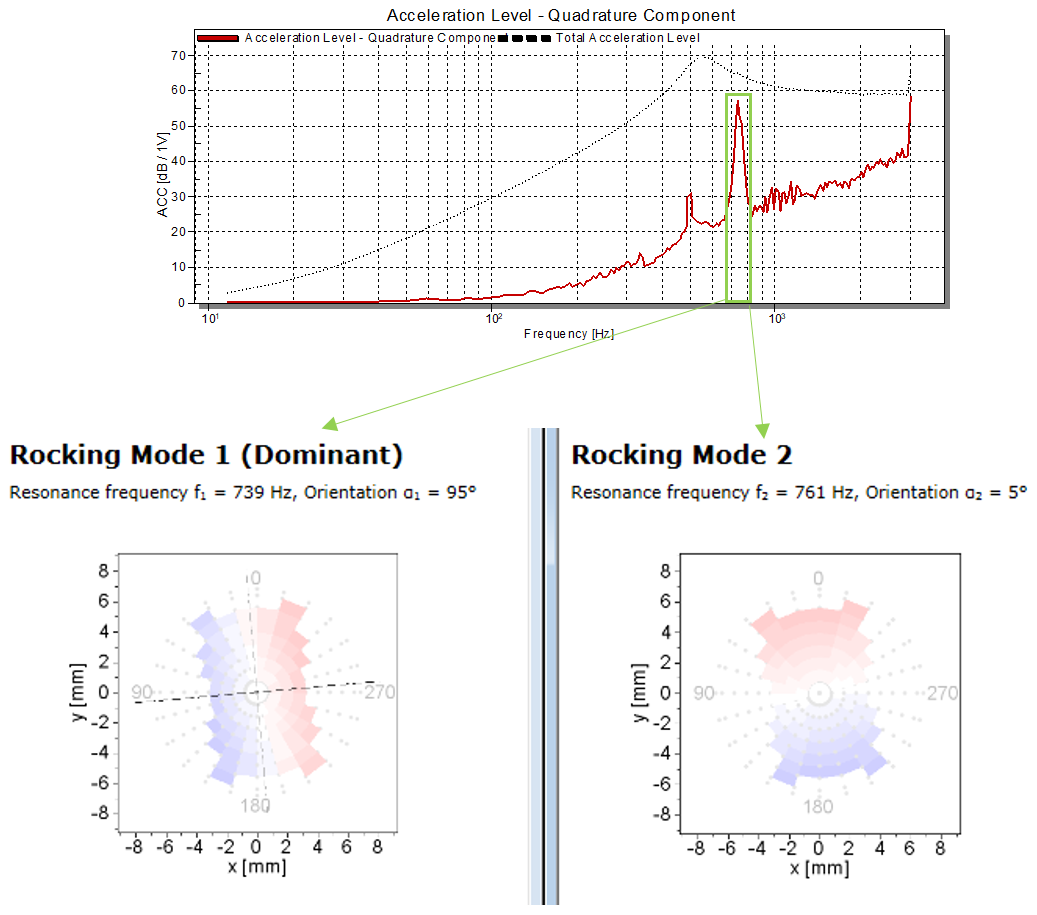
In the example above, both rocking modes are clearly identifiable, at 739 Hz and 761 Hz. Together they form the quadrature component in the SCN software. The rocking resonance frequencies f₁ and f₂ shall be close to those that you find in the SCN. In some cases, RMA will be able to detect separate resonances that are not visible as separate peaks in the AAL plot the SCN software, due to the resolution of its frequency axis.

Open the output windows AAL Rocking Mode 1 and 2

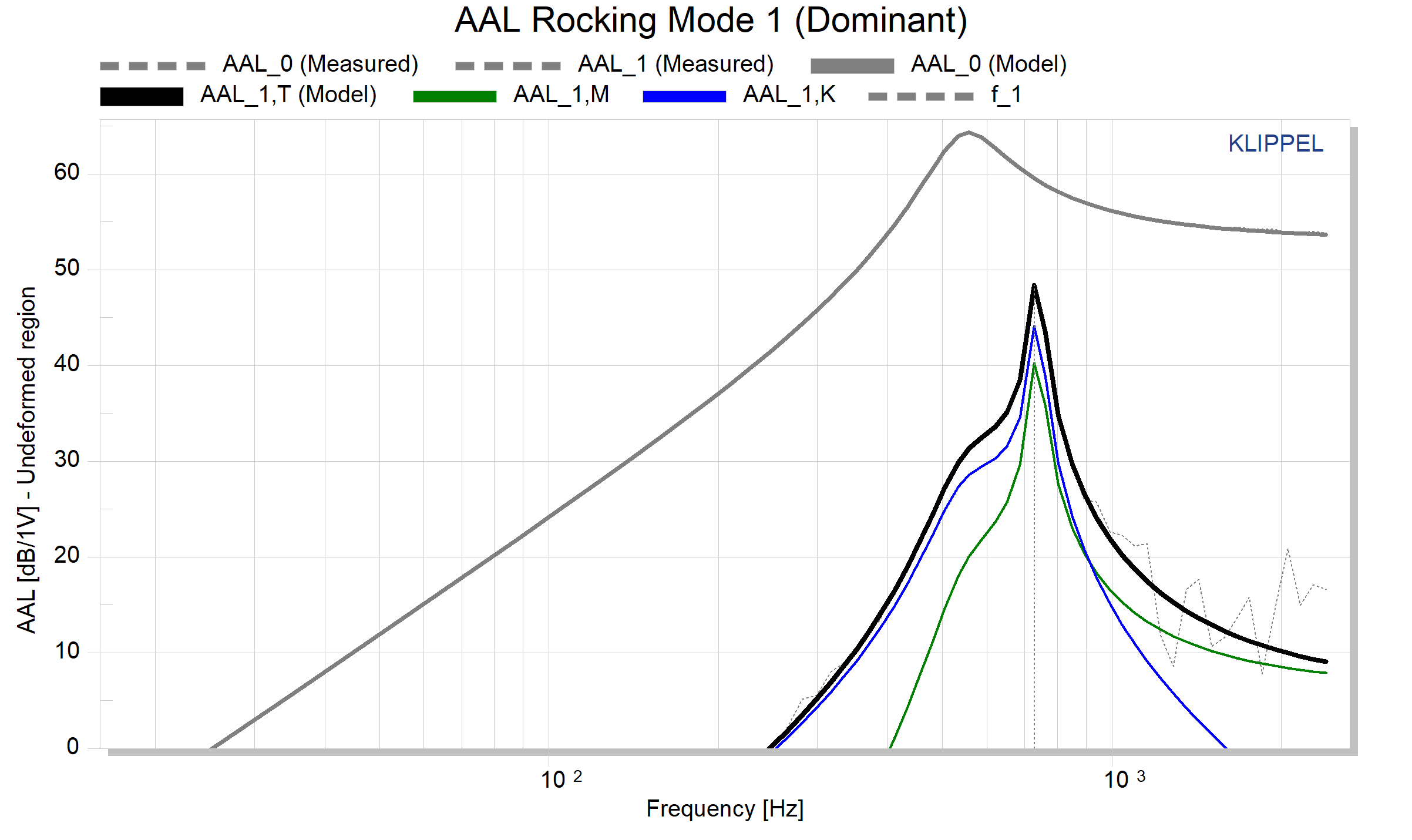
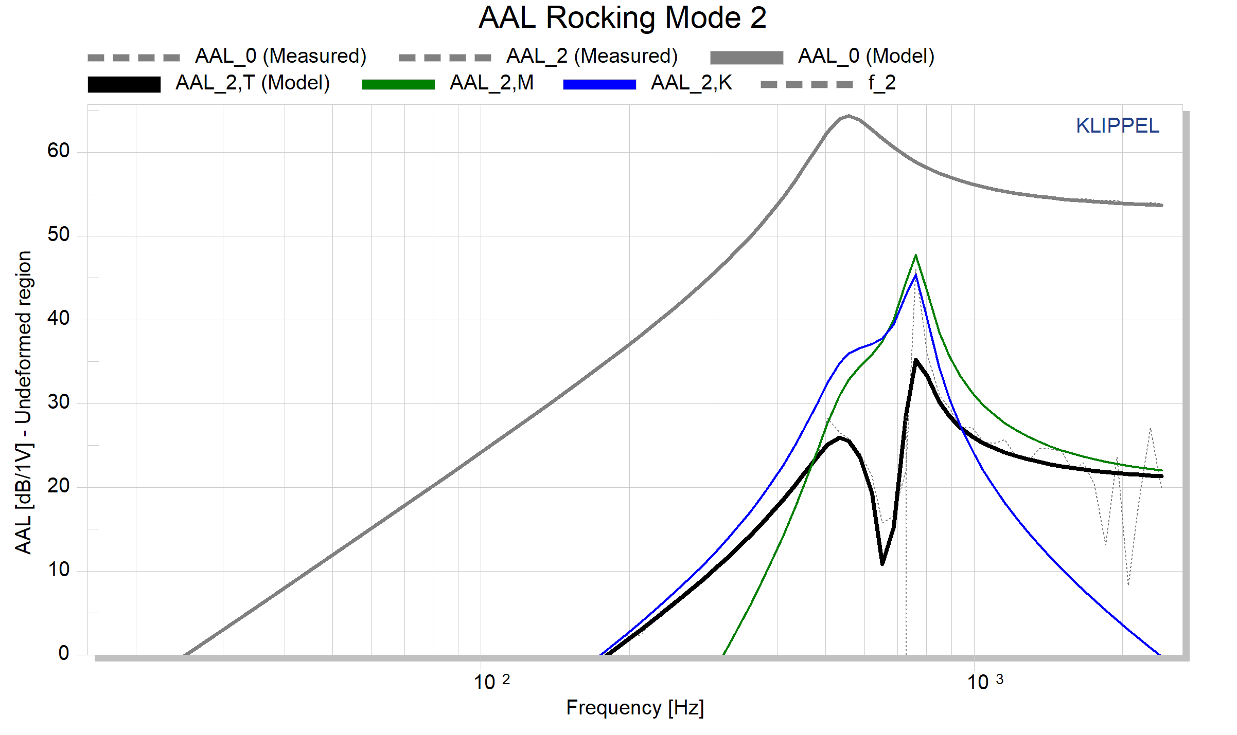
This result window shows the fitting of the model and the measurement for the piston mode of both rocking modes. The Accumulated Acceleration Level AAL₀ (see SCN documentation) corresponds to the piston mode characterized by the linear parameters of the driver. The AAL₁ and AAL₂ correspond to the first and second rocking modes that are identified with the RMA by adjusting the free parameters of the dynamic model. The total modeled curve AAL_T corresponds to the total contribution of the AAL_M mass, AAL_K stiffness and AAL_Bl force factor. These terms are plotted in the respective colors for each physical entity mass (green), stiffness (blue) and Bl (red). Note that the curve for Bl might not be shown, if the algorithm has excluded that entity from identification. If the identification worked well, the AAL curves of the fitted model (thick black lines) match the measured curves (grey dashed lines) tightly.

Open the Fitted Phase window

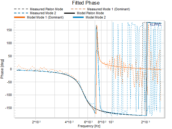
For the RMA, the correct phase fitting of the model variables is crucial for recognition of the physical problems presented in the measurement DUT (Device Under Test). This window shows the fitted phase of the identified model. Note that the differences between the model and the measured data should not be large below the resonance frequency of the driver.

Tutorial 3 - Understanding interaction of imbalances

This tutorial summarizes the interaction of different imbalances on tilting excitation of the diaphragm.

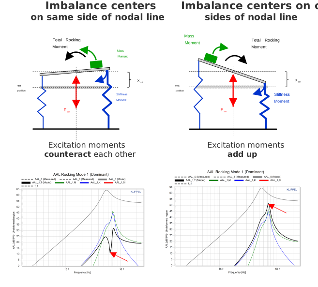
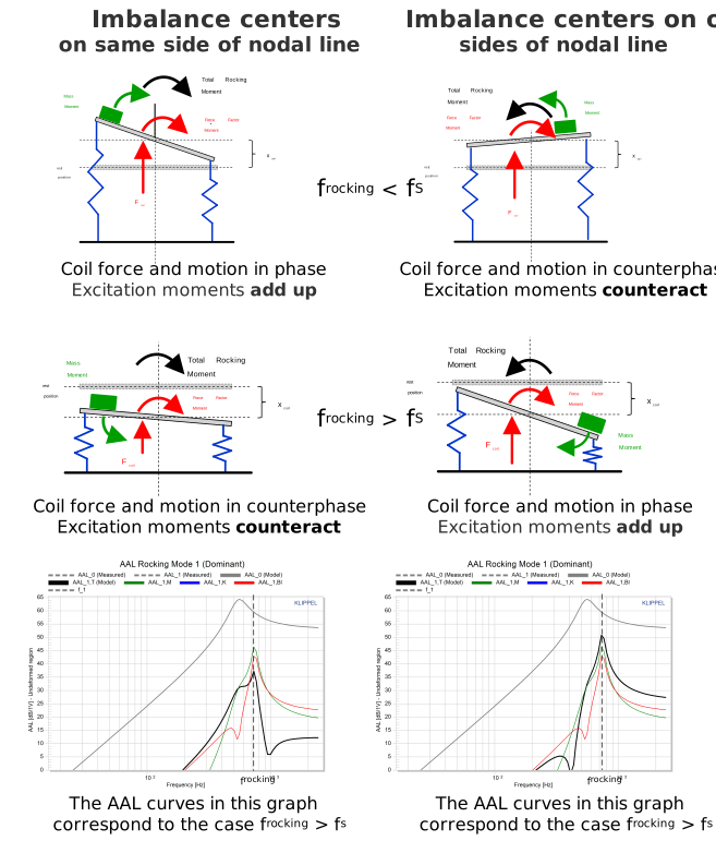
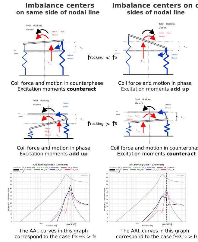
• The AAL curves show the constructive and destructive interference of the contributions from the different mechanical entities.

• The arrows in the motion diagrams correspond to the excitation moments acting around the rotational axis (=nodal line) of the mode.

To see a practical example from a real-life rocking case examined according to this information, please check the reference part of the manual in the section Modal Force Ratio MFR.

Mass and stiffness imbalances

Mass imbalances create rocking excitation forces that depend on the acceleration of the diaphragm (Force = mass * acceleration). Stiffness imbalances create rocking excitation forces that depend on the displacement of the diaphragm (Force = stiffness * displacement). Acceleration and displacement are always 180 degrees out of phase (=opposite sign) both below and above fundamental resonance of the loudspeaker transducer.

Mass and Force Factor (Bl) imbalance

Note

Since the excitation terms or moments of the mass and stiffness are proportional to the fundamental displacement (piston mode), the phase change depends on the fundamental resonance frequency of the driver. This effect is important when one of these two root causes interacts with the Bl term. The total contribution can produce adding or cancelling moments which respectively will increase and decrease the total excitation of the rocking mode below or above f_s.

Stiffness and Bl-imbalances

Note

Since the excitation terms or moments of the mass and stiffness are proportional to the fundamental displacement (piston mode), the phase change depends on the fundamental resonance frequency of the driver. This effect is important when one of these two root causes interacts with the Bl term. The total contribution can produce adding or cancelling moments which respectively will increase and decrease the total excitation of the rocking mode below or above f_s.

Reference

Measurement technique

The displacement in distributed membrane points measured by the laser scanner is the basis for modal analysis showing the direction of the two rocking modes represented by mode angles α₁ and α₂. The free parameters of the lumped parameter model in the modal space are estimated by minimizing the error between measured and simulated data.

General Schematic of RMA

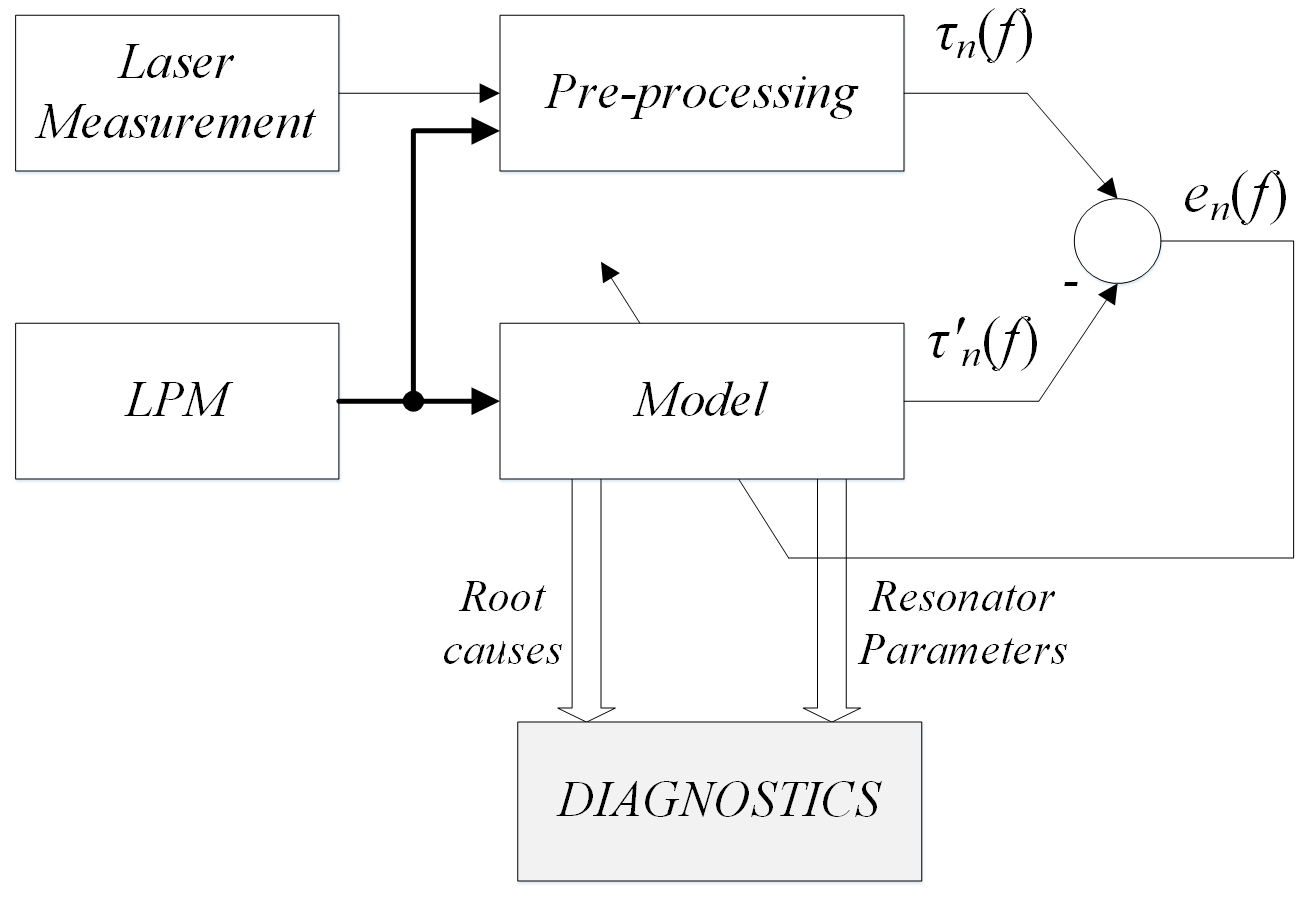
The pre-processing block performs a data reduction: It fits an oscillating plane onto the distributed measurement points, which extracts the rigid body motion component and allows to describe the rocking motion by a set of three modal oscillators. This process provides the measured state variables x_coil, τ₁ and τ₂ (displacement of the piston-mode and tilting angles for the two rocking modes). Using the LPM, RMA removes the excess of phase present in the measured data.

The dynamic model estimates the corresponding simulated states variables x’_coil, τ’₁ and τ’₂ by adaptive adjusting of the model parameters. The difference in magnitude and phase between the measured tilting angle τ_n and the modeled τ’_n is called error e_n (f). This error is minimized for each parameter.

Finally, the model provides two outputs: 1) The excitation terms µ_n,M, µ_n,K, µ_n,Bl describing the tilting moments acting onto the modelled modal resonators. 2) The modal resonator parameters (resonance frequency and damping of the lumped modal resonators. Together they form an ideal diagnostic tool to describe the excitation and response of the rocking modes.

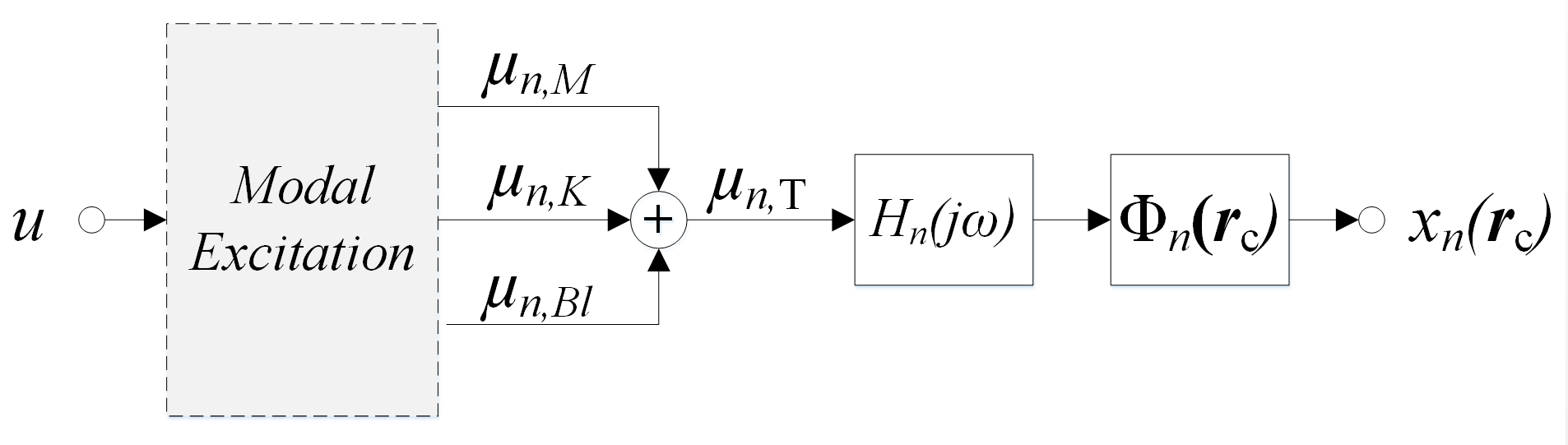
The root cause analysis requires the displacement X_T(jω,r_c) measured with sufficient local resolution at a multitude of points located on the diaphragm surface S_c. This scanning process may be performed providing amplitude and phase information with sufficient spectral information to identify the natural frequency and loss factor with sufficient accuracy. The generation of the rocking modes is described as a modal excitation. The excitation is generated by unbalances in the stiffness, mass and Bl. These imbalances produce the moments µ_n,K, µ_n,M and µ_n,Bl respectively. These tilting moments are added and boosted up with the modal transfer resonator H_n(jω) and produce then the output tilting (transversal displacement). The mode-shape

\[\Phi_{n}\left( r_{c} \right)\]

translates the lumped displacements and tilting angles (caused the mode with index n) into displacement values x_n(r_c) caused by that mode in every point r_c on the surface of the diaphragm. The subindex n = 1,2 denotes the first or the second rocking mode and n = 0 states for piston mode.

Inputs

Distributed Diaphragm Vibration Data (SCN)

Distributed vibration data shall be provided in Klippel SCN format.

Data measured with the Klippel Scanning Vibrometer System SCN shall be exported to *.sce file format by the using the option “Export>Export ASCII> [Geometry Format: Polar grid, Export Grid Points: Interpolated Data (original grid)]. These exported files will contain a full dataset of geometry and vibration data. Files of type .sce with very small size (< 0.1MB) that are not exported this way only contain links to other data files and no complete dataset as required by RMA.

Valid .sce files can also be gathered from other sources using the bridge modules for the Klippel Analyzer System. For data generated with a Polytec LDV, use the dB-Lab module Poly2SCN. See the RMA Specification for more information.

SCN data can be either referenced through specification of the path to the .sce-file or more conveniently by linking an SCN Data Container operation containing the data. The latter option is recommended, since it includes all source data into your dB-Lab database so that it cannot get lost.

Linear T/S Parameters (LPM)

RMA needs a set of linear (“Thiele-Small”) transducer parameters. Especially important are correct values of the electrodynamic coupling factor at rest position Bl, the moving mass Mms and the electrical resistance. Even the overall suspension stiffness linearized for the small-signal range is required with reasonable accuracy. The most accurate and convenient way to gather this data is to perform a linear parameter measurement with Klippel LPM and to link the respective LPM operation to RMA. Choose “Klippel LPM/FEM2SCN”-Operation as T/S Parameter data-source to use this option. Users of our bridge-module Poly2SCN can alternatively provide T/S parameters by hand. Clipboard import from LPM operations is also supported.

Diaphragm Geometry

Select the general diaphragm shape from the dropdown list: Circular, rectangular or ring.

Rigidly Oscillating Diaphragm Dimensions

Rigidly oscillating radius (for round transducers) or half-length and half-width (for rectangular transducers). All of these shall describe only the diaphragm area that is vibrating as an undeformed plate. This means that all parts that suffer major deformation within the analysis frequency range (like e. g. the surround) have to be excluded here.

Processing Frequency Limits

Define the frequency range [f _min f _max] that includes the fundamental piston resonance and rocking resonances. If not corrupted by noise or breakup-modes (vibration behavior where the center part of the cone suffers from major deformation), include also two octaves above and below any of these resonances.

f _min = lower frequency limit

f _max = upper frequency limit

Computation Speed [optional]

Value to reduce the number of frequencies included in the analysis to decrease the computational time.

• Fast = Much less frequency points (Q-factors will not be fitted accurately). If the scanned data is of extremely high (frequency-) resolution (no frequency log reduce selected in TRF settings of SCN setup), then using this setting may be advantageous to avoid out-of-memory-problems of RMA. This setting reduces the size of the internally used vibration mesh if the original mesh is larger than 140 points.

• Normal = Slightly reduced number of frequency points. This offers a compromise between speed and accuracy. A good standard setting that works well almost always. This setting also reduces the size of the internally used vibration mesh if the original mesh is larger than 140 points.

• Slow = All frequency points. Use this setting for most accurate identification of Q-factors. The calculation of results will take more time. This setting also deactivates any geometrical data reduction.

Advanced Settings [optional]

• Exclude Frequency Range: Allows the user to exclude sections from the analysis frequency range that was selected under Processing > [fmin, fmax]. This can be useful to avoid that any artifacts caused by noise or breakup-modes are affecting the results.

• Show Parameter Explanations: Activating this option will display short descriptions in empty result windows explaining the parameters shown there. The descriptions are only visible as long as the operation is not executed and result windows are “empty”.

• Extract Diagrams: When activated the Summary and Rocking Mode 1/2 windows will be split after calculation resulting in the tables and the plots being in separate windows.

Outputs

Summary

The window Summary combines the most important outputs of RMA giving a sequential answer on the questions:

• How large is the Rocking Mode problem? > Relative Rocking Levels RRL. The given severity scale is based on rules of thumb and shall only serve as a rough orientation. How severe the rocking is in detail, depends on the DUT- its use-case, its geometrical design and the requirements. The gradings given here are defined by the RRL of each mode as follows:

  • > -6dB => “High”

  • > -12dB => “Elevated”,

  • > -18dB => “Moderate”,

  • < -18dB => “Low”.

  The link “Details” in the RRL table leads to a detailed view on the collected parameters of the respective mode. > Details Rocking Mode 1 and 2

• Which physical parameter causes the largest excitation force of the rocking motion? This decides which effect is dominant. To improve your driver, treat the dominant effect first before addressing the other contributions. > Combined Force Ratio.

• Where on the diaphragm is the root cause located? > Imbalances

An introduction how to navigate through the different result parameters of RMA in a meaningful way is given in Tutorial 1 – Viewing the results.

Details Rocking Mode 1 and 2

The windows Rocking Mode 1 and 2 provide an overview on all information that RMA has gathered on each mode separately. On top of the window, a visual representation of the modeshape shows in which direction the tilting is oriented. The angles α₁ and α₂ denote the direction of the maximal tilting of the rocking modes. This angle is perpendicular to the rotation axes of the rocking modes and referenced to the coordinate system labeled in the scanner turn table. At the same time the grey points in the background indicate the measurement points of the SCN data. The grey numbers reference the angles on the turntable of the Klippel Scanning Vibrometer System SCN.

Then, the information about the rocking mode is structured in three sections, answering the questions

• How large is the Rocking Mode problem? > Relative Rocking Levels RRL. These are split up into the contributions of mass, stiffness and force factor Bl. Some parameters may be inactive, if they were identified as minor for the overall result or if they could not reliably be determined. The link “Details” in the head of this section leads to the representation of AAL Rocking Mode n.

• How strongly is the rocking mode excited? > Modal Force Ratio MFR

• Characterization of the rocking modes in physically meaningful parameters. A second order system like this is completely defined by a set of modal parameters, which are collected in the Modal Parameter Tables

AAL Rocking Mode n

The Accumulated Acceleration Level AAL is a known Klippel parameter used to describe the mechanical energy on the surface of the diaphragm, as defined in IEC 60268-22

\[\text{AAL}(f,r_a) 20\log_{10} \left( \frac {\rho_0\omega^2} {2\pi\sqrt{2}p_0} \int_{S_c}^{} \left| \frac {H_{X/U}(r_c)\cdot1\text{V}} {r_a-r_c} \right| \text{d}S_c \right)\]

for a frequency f, a response point r_a in the sound field (here referenced to 1 m on axis), electromechanical transfer function H_X/U (surface displacement X / excitation voltage U) and diaphragm point r_c at reference excitation voltage 1V.

The AAL can be understood as the maximum theoretical sound pressure output of a loudspeaker, if all points of the diaphragm would vibrate in phase, at 1m distance on axis for 1V excitation voltage.

The AAL_i describes the output of the rocking resonator of each mode i. RMA also computes the AAL_n,E related to each root cause E (mass, stiffness or Bl).

The AAL clarifies the interaction between the root causes in the spectrum. The adding (dominant mode) and cancelling (nondominant mode) effects caused by the superposition of the excitations can be seen. AAL can be interpreted as a kind of frequency response of the final tilting produced by each root cause. For instance the stiffness is active at low frequencies and the mass dominates at high frequencies.

The AAL is also suitable to visualize the transfer characteristics of the rocking resonators displayed in the lower section of the Modal Force Ratio MFR result windows.

Practical application (microspeaker tutorial example): For the driver in the example below, the Q-factor of the dominant and nondominant modes are 32 and 45 respectively.

Relative Rocking Levels RRL

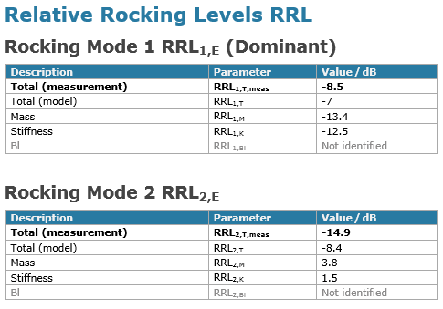
Relative rocking Level (RRL) is one main RMA result used to describe the severity of the rocking problem, describing the relevancy of a particular rocking mode. It is calculated as the dB difference between the piston mode (AAL₀) and the rocking modes (AAL_n,E).

\[RR{L_{n,E}}({\omega _n}) = AA{L_{n,E}}({\omega _n},{{\bf{r}}_{\rm{a}}}) - AA{L_0}({\omega _n},{{\bf{r}}_{\rm{a}}})\]

AAL_n,E can denote either all root causes combined (T) or the separated imbalances of mass (M), stiffness (K) and force factor (Bl). Note that the relevant value is the total one, since the cancellation effects produced by the superposition of the excitation terms, can lead to huge values of RRL for the independent root causes. RMA internally relies on the measured total RRL. Due to the very high Q-factors of rocking modes, very small mismatches of model and measured data can cause large differences in the peak values of the resonators. For this reason, the readings of measured and modelled RRL can deviate with up to 4 dB. The RRL values that are reproduced in the RMA result window Summary are the measured values.

Practical application (tutorial microspeaker example): | The total RRL_1,T,meas (dominant) of rocking mode 1 is measured with -8.5 dB, which describes the relation between the mechanical energy associated to the dominant rocking mode and the piston mode at resonance frequency of rocking mode 1. It can be seen that the corresponding values for mode 2 are much smaller.

The results are accessible for automation export through the following result variables

Modal Force Ratio MFR

The modal excitation ratios MFR_n,E, describe the equivalent asymmetric excitation forces that are acting perpendicularly to the rotational axis of the mode. These forces are calculated by translating the tilting moments µ into forces positioned at a reference distance from the pivot point for the tilting. These forces include both the direct excitation terms as well as the intermodal coupling terms. The reference distance d_ref is directly related to the diaphragm geometry defined by the user in the property page of the RMA. For a circular geometry, d_ref is the given radius of the rigidly oscillating part of the diaphragm r_rigid, for a rectangular geometry it is defined equivalently by the longer of the two parameters “rigidly-oscillating half-length” and “rigidly-oscillating half-width” from the input property page.

\[F_{n,E} = \ \frac{\mu_{n,E}}{d_{\text{ref}}}\]

F_n,E here is the equivalent force of the tilting moment µ_E calculated for reference distance dref. The subindex E stands for any of the physical entities mass (M), stiffness (K) or force factor (Bl).

\[\left| {MF{R_{n,E}}} \right| = \frac{{\left| {{F_{n,E}}\left( {{f_n}} \right)} \right|}}{{\left| {{F_0}\left( {{f_n}} \right)} \right|}}\]

for mode n=1,2 and E ∈ {M,K,Bl}

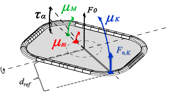
The MFR is useful to evaluate the magnitude of the tilting moments that are caused by each physical effect at the rocking resonance frequencies. Since these moments are mathematically described by a multiplication of the size of the imbalance with one frequency-dependent state variable (mass with acceleration, stiffness with displacement and Bl with current), the MFR allows to rank which physical contribution (mass, stiffness or Bl) creates the largest excitation for the rocking. The magnitude of the excitation moment is what is finally important for ranking the different root-causes, irrespective of which physical contribution has the largest Imbalances. Expressing the excitation moments as forces and comparing them to the piston mode force is useful to get a feeling for their magnitude.

Practical application: The Modal Force Ratio MFR_n for cases with only mass and stiffness considered in the fitting, the interpretation of the RMA results can be seen as a simple 2D system. The absolute value of the Modal Force Ratio 1 gives an indication of which root cause inducest the largest excitation force at rocking resonance in the direction of motion for mode 1. The below analysis is done for the tutorial microspeaker example. We begin with the dominant rocking mode 1:

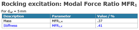
The absolute value of the modal force ratio indicates that the stiffness contribution is slightly larger than the mass contribution for mode 1, though they are of very similar magnitude. To understand the effect of this, we need to consider in which direction these forces are acting.

Mode shape of rocking mode 1

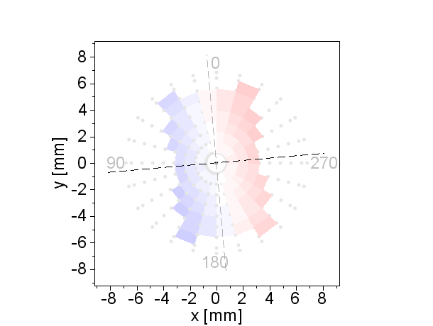
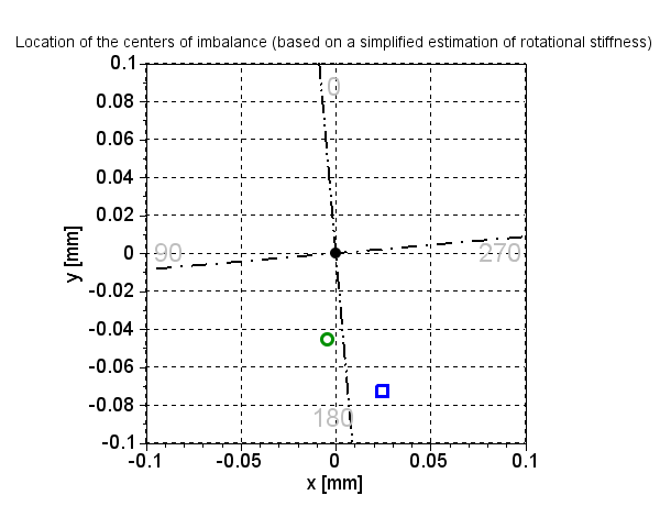
For mode 1, the centers of the distributions of mass and stiffness are on different sides of the nodal line around which mode 1 rotates. The centers for mass and stiffness lie close to the nodal lines which triggers only small imbalance forces <1% as shown by the MFR₁. In the next step we shall analyze the phase of these forces to determine whether they add up or cancel each other.

The respective case can be found in the tables given in Tutorial 3 - Understanding interaction of imbalances.

For mode 1, the excitation moments of mass and stiffness add up constructively.

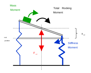
We can conclude for rocking mode 1 that the moments induced by the stiffness and mass imbalances are both turning the diaphragm in the same direction “clockwise”, when the symmetric voice coil force F_coil acts on the driver. For this reason the total contribution is larger since both moments are adding to each other which increase the rocking. The resulting excitation force is 0.37 [%] + 0.41 [%] = 0.78 [%] of the excitation force from the piston mode.

Doing the same analysis on the Modal Force Ratio MFR of the secondary mode:

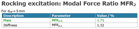
Here the absolute values of the Modal Force Ratio are again of similar magnitue with the mass contribution being slightly larger. Note that the absolute values of the contributions are three times as large as for the dominant rocking mode 1.

Mode shape of rocking mode 2.

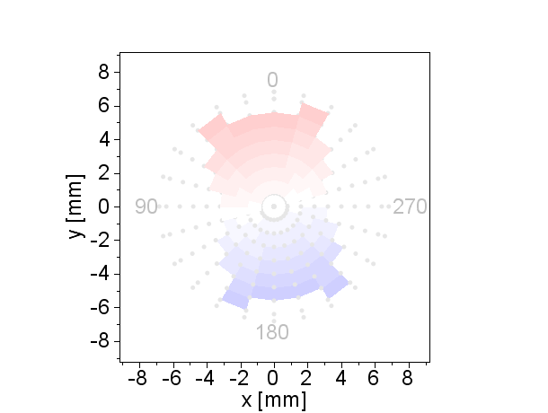
For mode 2, the centers of the distributions of mass and stiffness are on the same side of the (dotted) nodal line around which mode 2 rotates. The MFR shows the magnitude of the forces that arise from this. In the next step we need to consider their phase.

The respective case can be found in the tables given in RMA Tutorial 3 for interpretation of the physical results.

For mode 2, the excitation moments of mass and stiffness substract from each other and almost cancel out.

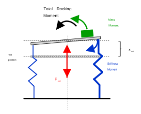
It can be seen that the mass and stiffness imbalances are compensating each other which leads to a rocking mode with less excitation than if each physical effect (mass or stiffness imbalance) would have been present alone. The resulting modal excitation force for mode 2 is 1.71 [%] -1.32 [%] = 0.39 [%] of the voice coil force.

The above analysis explains why the rocking mode 1 is the dominant one in the microspeaker tutorial example. Although the excitation forces that each physical entity contributes with are three times as large for mode 2 compared with mode 1, the final combined resulting excitation force of mode 1 is double the magnitude of mode 2. The effects that this has on the rocking levels can be observed in the result windows Relative Rocking Levels RRL and AAL Rocking Mode n.

The values of MFR obtained for both modes are joined together to the Combined Force Ratio CFR which describes the global excitation of both modes a common “middle-frequency” between the modes. The MFR is part of the RMA result window Details Rocking Mode 1 and 2.

The results are accessible for automation export through the following result variables

Combined Force Ratio CFR

The Combined Force Ratio (CFR) reveals the excitation of both rocking modes combined together. It is calculated at the geometrical mean value of the natural frequencies f₁ and f₂ of the two rocking resonances.

\[{f_{\rm{m}}} = \sqrt {{f_1}{f_2}}\]

It is defined as the relation of the excitation of both rocking modes and the excitation of the fundamental mode. The CFR considers only the primary moments μ_n,E(f_m) (proportional to x_coil) with n = 1,2 and. This means that the contribution of the modes is added up vectorially and individually, neglecting any secondary excitation that can be caused by the influence of the modes on each other.

\[\left| {{\rm{CF}}{{\rm{R}}_{\rm{E}}}} \right| = \sqrt {{{\left| {{\rm{MF}}{{\rm{R}}_{1,{\rm{E}}}}\left( {{{\rm{f}}_{\rm{m}}}} \right)} \right|}^2} + {{\left| {{\rm{MF}}{{\rm{R}}_{2,{\rm{E}}}}\left( {{{\rm{f}}_{\rm{m}}}} \right)} \right|}^2}} = {\rm{\;}}\frac{{\sqrt {{{\left| {{{\rm{\mu }}_{1,{\rm{E}}}}\left( {{{\rm{f}}_{\rm{m}}}} \right)} \right|}^2} + {{\left| {{{\rm{\mu }}_{2,{\rm{E}}}}\left( {{{\rm{f}}_{\rm{m}}}} \right)} \right|}^2}} }}{{\left| {{{\rm{F}}_0}\left( {{{\rm{f}}_{\rm{m}}}} \right)} \right|{{\rm{d}}_{{\rm{ref}}}}}}\]

with the reference distance d_ref, the Modal Force Ratio MFR and the voicecoil excitation force F₀ that is driving the pistonic motion.

Practical application: The Combined Force Ratio CFR_E informs us about how strong the excitation terms are relative to each other and relative to piston mode. This allows us to specify the excitation effect (mass, stiffness or Bl imbalance) that causes the dominant excitation. In case that there is one clearly one dominant effect, improving this one is most beneficial in order to improve the rocking performance of the driver.

Example 1:

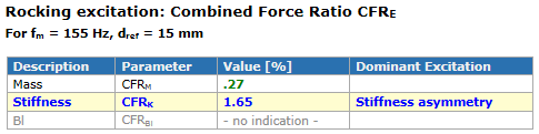
For this microspeaker (another one than the usual tutorial example), the root cause exciting the dominant rocking mode is a 1.65 % stiffness asymmetry.

The rocking problem in this driver shows only a minor influence of a secondary root cause, which is a 0.27% mass imbalance.

Note

For drivers with several rocking root-causes at similar level, the interaction (phase relation) between the several imbalances needs to be studied first. For this you can rely either on the imbalance plot or on the AAL graph. Guidance on physical interpretation of the occurring effects is given in RMA Tutorial 3.

Modal Parameter Tables

The following parameters describe the rocking resonators H_n(jω)

The relative gain of the transfer function between the equivalent excitation force F_n,T and the total value AAL_n,T defined by

\[R{G_n} = AA{L_{n,{\rm{T}}}}({f_n}) - AA{L_0}({f_n}) + 20{\log _{10}}\left( {\left| {\frac{{{F_0}({f_n})}}{{{F_{n,{\rm{T}}}}({f_n})}}} \right|} \right)\begin{array}{*{20}{c}}{}&{}&{n = 1,2}\end{array}\]

Is a valuable characteristic to assess the behavior of each modal resonator with n = 1,2 at the natural frequency f_n. The damping factor η_n and the Q-factors Q_n are derived based on the -3 dB rule around the resonance peaks.

The Modal Parameter Tables are part of the RMA result windows Details Rocking Mode 1 and 2.

Fitted Resonator Phase

The phase of the resonators describing the displacement of piston mode and both rocking modes relative to the measured excitation voltage.

Imbalances

The three physical effects that RMA can distinguish as root causes for the rocking (uneven distributions of mass, of stiffness and of electromagnetic force factor) are described by the coordinates of the centerpoints of their distribution, when lumped together into one point. For example, the mass distribution over the diaphragm is represented by the amount of lumped moving mass together with the coordinates of the center of gravity. In analogous ways this is done for stiffness and Bl factor as well. In all situations where this lumped parameter center-coordinate deviates from the geometrical center of the diaphragm, the piston mode that moves the diaphragm in and out will induce a non-axisymmetric force that causes a tilting momentum. This drives the rocking motion. The offset of the center of lumped parameter distribution from the geometrical center of the diaphragm is called “Imbalance”. It describes the root cause for the rocking.

The result is presented as table and imbalance center diagram in the dB-Lab window RMA Result. Here this is visualized for the microspeaker from RMA tutorial 2:

Imbalance center diagram

Mode shape of rocking mode 2

Mode shape of rocking mode 1

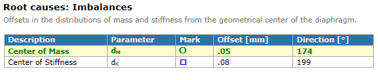
The main axis of modal rocking motion is indicated with a single-dotted line for mode 1 and a double-dotted line for mode 2.

The absolute magnitude of the imbalance (measured in millimeters) is directly proportional to the absolute value of the mechanical rocking mode parameters - rotational stiffness and rotational inertia of the DUT around the rocking-axes. These cannot be measured by RMA in absolute terms. Since rotational stiffness and rotational inertia are interrelated by the rocking resonance frequency, we can use any of these two as a scaling factor to obtain absolute imbalance values. RMA uses the rotational stiffness around each of the main axes of rocking motion for this scaling. This rotational stiffness is in turn highly dependent on the geometrical and mechanical design of the DUT and not a-priori available for RMA. This is why RMA will only provide results for imbalance relative to rotational stiffness. If required, this result can be converted to absolute values by multiplying with an accurate estimate of rotational stiffness. In this way RMA and Finite Element Modelling can work closely hand-in-hand: RMA will provide the asymmetries of distribution of mechanical diaphragm parameters that cannot be simply estimated a priori by numerical modelling. However, FEM can simply estimate rotational stiffnesses, which is not possible accurately with the simple set of input parameters that are accessible by RMA.

Note

The imbalance diagram shown in the window “RMA result” is only a rough estimate of the absolute coordinates of the imbalances.

For the imbalance diagram generation the rotational stiffness around the axis of motion for rocking mode index i is very roughly approximated by

\[K_{\tau,i} = \ \frac{d_{ref,i}^{2}*K_{\text{ms}}}{2}\]

where K_ms is the axial mechanical stiffness of the driver suspension provided by LPM and d_ref,i is the rigidly oscillating dimension in the respective direction i as defined under “Diaphragm geometry” in input property page tab “Setup”.

Errors / Warnings

RMA features a thorough assessment of the quality of its result. In case that this triggers an error or warning case during the processing, the respective message will be shown in the upper part of the window under “Info/Warnings/Errors”. Errors will be shaded with red background color and warnings in light orange. In the section “Information” of the table, the processing settings for laser delay, amplifier gain, T/S datasource and special frequency range settings are displayed.

The second section “Result Quality Assessment” provides a grading of the trustworthiness of the subsequent steps of RMA analysis. Note that the word “error” in the context of quality assessment has a different meaning than above. We do not refer to a misfunction here, but to a “fitting error” which is usually defined as a relative deviation of modelled from measured data, given in percent. A certain percentage of error is normal for a tool relying on fitting methods applied to low-energy data. The grading steps provide guidance whether the analytic results are of sufficient quality.

For all fitting error types described below, the following verdict classes are used

Verdict	Error percentage range
Good	0 - <12
Sufficient	12 - <24
Poor	24 - <36
Insufficient	>36

The overall quality of RMA identification is described by the lowest ranking of the identification chain. In cases where this value falls in verdict ranges “poor” or “insufficient” your RMA results should be considered inaccurate.

Hint

To resolve problems, consider the advice given in the warning messages in the Errors/Warnings window (note that the advice can be expanded by clicking on the links marked “>>>”) or check the chapter RMA Troubleshooting. The defined error-measures are defined in separate sections below.

Spatial SCN plate-fitting error

The spatial SCN plate-fitting error E_SCN indicates how well the selected part of the diaphragm can be described by a rigid plate. The error measure is defined as twice [11] the RMS sum percentage over all processing frequencies of the residual from fitting a perfect plate to the measured displacement of the selected undeformed central part of the diaphragm.

[11]

The factor two is introduced to scale up the severity of this error, considering that any error in step 1 of the RMA process will negatively affect accuracy in all subsequent steps of the analysis, which also have proven to be quite sensitive for inaccuracies in the platefitting.

This process is only accurate if the deformed parts of the diaphragm are excluded from RMA evaluation. The points included in this fitting are contained inside the diaphragm area specified by the user as the rigidly oscillating half-length, half-width or radius parameters, depending on the kind of geometry. But, also the frequency ranges play an important role.

The most common mistakes causing problems are:

• Parts of the surround area which suffer from major deformation are included in the definition of the diaphragm geometry in RMA setup. See section Assessing valid geometrical dimensions

• The evaluation frequency range is too wide. This can be changed in section Processing frequency settings in the RMA setup.

  • The upper end frequency fmax too high: The analysis reaches frequencies where the diaphragm already starts to bend in the middle part due to “breakup-modes”. This can easily be detected with an animation in the Klippel Scanner System analysis software.

  • The lower end fmin is too low: Frequency points with major influence of measurement noise are included in the evaluation. This is though rather rare if the correct stimulus shaping is used in the SCN measurement (See step 8 of Tutorial 2 Measuring LPM and SCN input data for RMA)

• Corrupted measurement points with unphysical behavior are present in the SCN data. Learn how to remove corrupted points in Tutorial 2, section Preparing SCN data for use with RMA module

Piston Mode Fitting Error

The piston mode fitting error E_Piston expresses, how well RMA was capable to fit linear parameters describing the piston mode to the rigid body vibration read from the scanner data. RMA will compare the result to the T/S parameters provided a-priori by the user and give a warning if major deviation occurs. The error measure is defined as the RMS sum over all frequency points of the modelling residual. It is given in percent and increases if the dimensions of the diaphragm are too large or if there are any phase errors. To avoid this, check that RMA has estimated a meaningful laser delay.

Rocking Mode Modeling Error

After the system Identification is finished, the model with the optimal parameters will resemble the measurement as much as possible, but still show some deviation. For RMA, accuracy in magnitude and the phase modelling are equally important since they respectively provide information about how critical a rocking mode is and what is the root cause. Both amplitude and phase accuracy are combined in the rocking mode modeling error E_Rocking reading, which is given in percent.

Interfaces to other modules

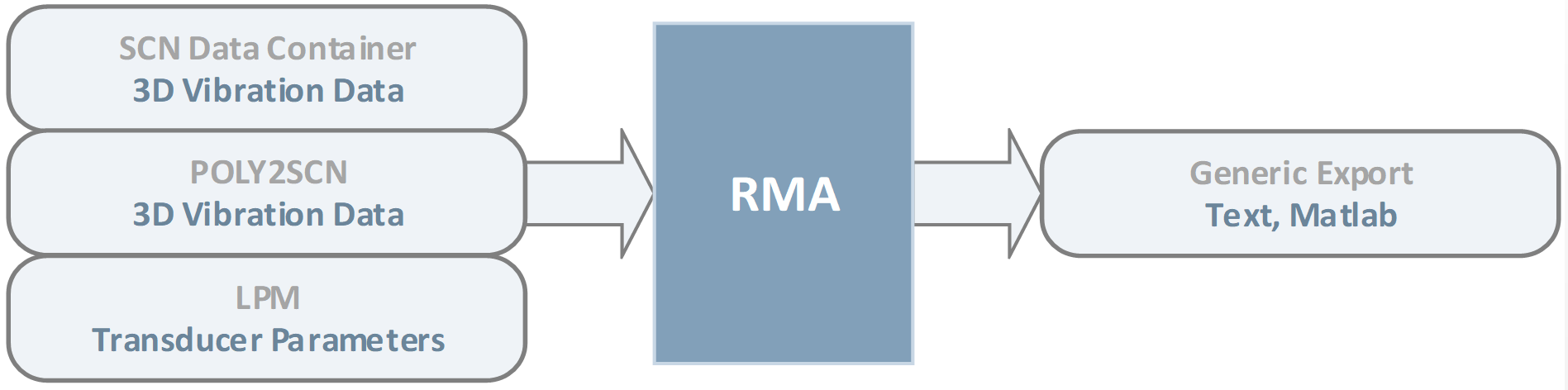
RMA requires both linear (“Thiele-Small”) transducer parameters and distributed vibration data. The former can be imported from a linear parameter measurement with Klippel LPM. (In addition, users of Poly2SCN are given the option to specify LPM parameters manually) The latter can either be measured with the Klippel Scanning Vibrometer SCN or with a Polytec LDV (data conversion via our bridge-module Poly2SCN). The preferred input format for distributed vibration data is the SCN data container. Though RMA will also read exported Klippel SCN files in .sce format.

RMA Troubleshooting

Most frequent problems

The error measures shown in result window Errors/Warnings describe the validity of the results. In the following examples, some possible errors originating from incorrect RMA settings will be analyzed. The examples will illustrate how errors can be detected and interpreted.

Wrong geometry dimensions

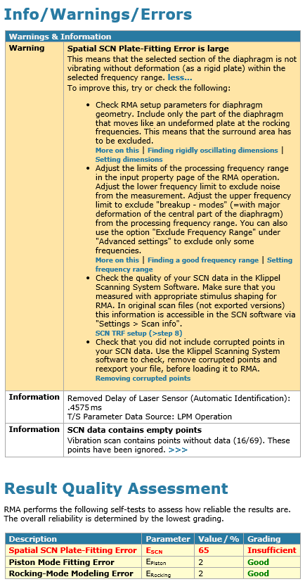
For this example of a rectangular driver, the settings for “Diaphragm Geometry” in input property page “Setup” are incorrect. Here, the measurement data that is selected for evaluation with RMA includes not only the rigidly oscillating part of the diaphragm (the area that moves like an undeformed plate), but also some points on the surround where deformation is large. In this special case, the user has mixed up the values for half-length and half-width and has specified them cross-wise (half-length value in the half-width field and vice versa). This includes a large part of the deformed surround region in the data that is selected for evaluation by RMA. The problem is highlighted by the Spatial SCN plate-fitting error appearing in red with a large error value. The associated warning message above provides additional hints about how this problem could be solved.

Caution

If the E_SCN error is close to zero, but the E_Piston is large, ensure that both of the scanner and the LPM measurements do not exceed the voltage range for linear operation of the DUT. Guidance for this can be found in step 2 of Tutorial 2 Measuring LPM and SCN input data for RMA

Note that if the dimensions of the rigidly oscillating part of the diaphragm (specified in property page “setup”) are too small compared to the correct value, this will affect the estimation of rotational stiffness of the driver which in terms will scale the absolute values for Combined Force Ratio, Modal Force Ratio MFR nd the estimation of radial distance of the center of imbalance from the centerpoint of the diaphragm. It will also affect all AAL levels and with that even RRL and the estimate of severity. Most of these values are found in result window “RMA results”.

Anyhow, some of the key results of RMA such as:

• which root cause (mass imbalance, stiffness imbalance or Bl imbalance) is the largest

• in which direction are the centers of imbalance located

will still be accurate if any of the following conditions is obeyed:

• the transducer geometry is round

• rectangular drivers: the ratio between “rigidly oscillating half-length” and “-width” is correct

Caution

A too large value for the rigidly oscillating diaphragm dimension is by far more severe for the RMA result than if the dimensions are specified too small. No parts of the surround area with major deformation may be included in the specified rigidly oscillating diaphragm dimensions. This is valid as long as a sufficient amount of points is available for fitting.

Wrong processing frequency range

Some important differences between the root causes of rocking modes can be found at frequencies below the fundamental piston resonance of the transducer. For RMA to identify these, that frequency range has to be included in the analysis.

Too narrow frequency boundaries:

In this example, the selected lower processing frequency limit fmin was 330 Hz, less than one octave below the fundamental resonance of the driver 540 Hz. A good practice is to choose the low frequency cutoff so that the maximum amount of frequency points is included, but avoiding noise. Usually, setting f_min = f_s/4 is a good choice. Though make sure not to include excessive measurement noise which might appear at very low frequencies. Also above the rocking resonances, the frequency range is too narrow in this first example and the root causes are hard to separate.

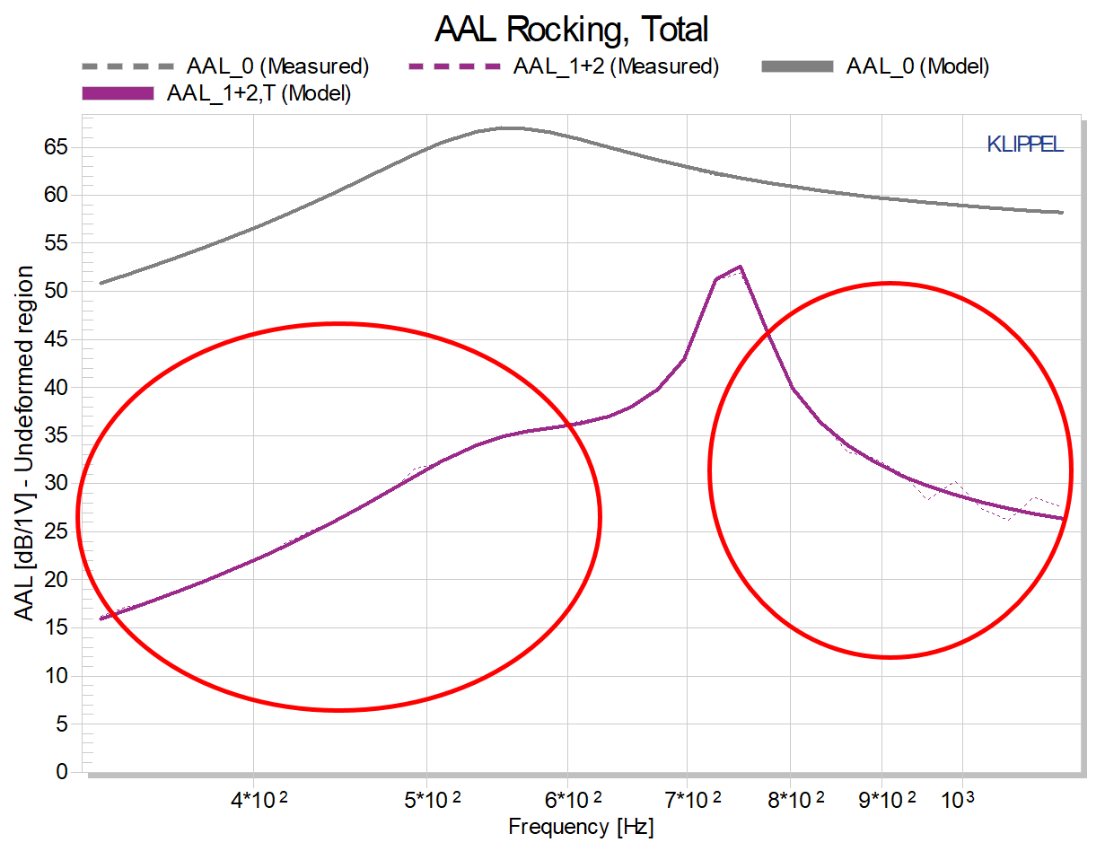
Too wide frequency boundaries:

In the second example, the high-frequency cutoff is chosen too high and the diaphragm breakup modes is included in the analysis frequency range. A large Rocking Mode Modeling Error indicates this. The reason for the occurring error is, that measurement data is getting corrupted by more high-frequent diaphragm-deforming modes (“breakup modes”). The frequency range where these dominate shall be excluded from the analysis frequency range.

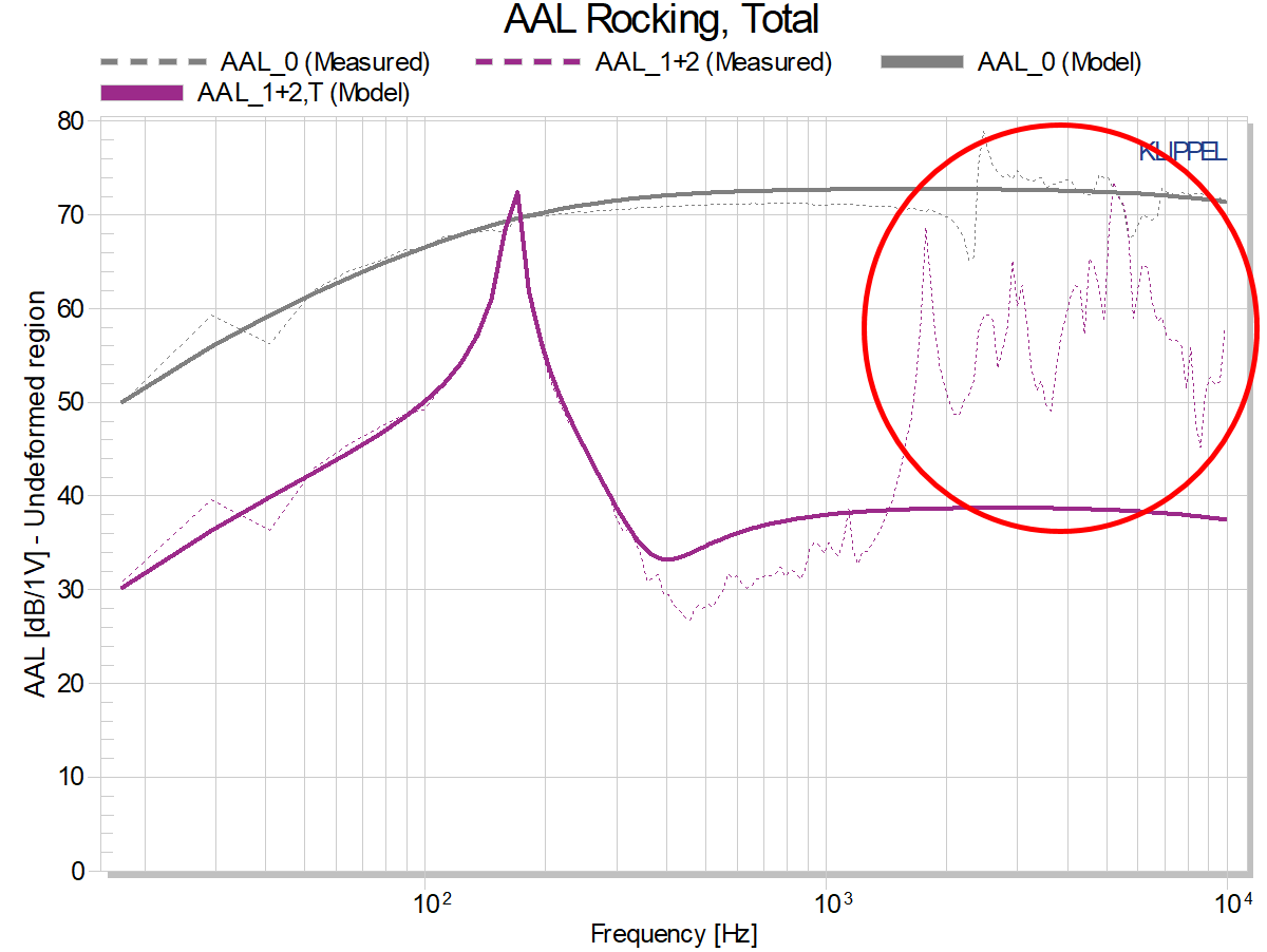
Hint

Choose the right frequency range

• Too narrow frequency boundaries = The root causes are hard to separate

• Too wide frequency boundaries = Breakup modes are included and causes plate fitting problems.

Too fast evaluation speed

RMA can run at different evaluation speeds. RMA omits frequency points at faster evaluation speeds. This may cause problems for finding the correct Q-factor of the modal resonators. The associated warning informs that the Q-factor was not found. You will even see a rougher fitting in the AAL curves, especially in the peak regions.

Noisy input data

Correct setup of the vibration scanning device is crucial for flawless operation of RMA. Excessive noise in the input data will make it impossible for RMA to achieve sufficient fitting quality of the distributed vibration data in amplitude and phase. Noisy input data can be easily identified by strong ripples in the curves displayed in result windows AAL Rocking, Total or Fitted Phase. Thorough guidance how to set up your Klippel Scanning Vibrometer in the best way for RMA is given in RMA Tutorial 2. Follow the description in step 8 to find a suitable stimulus voltage and shaping.

Errors in estimation of laser delay

A correct value for laser delay is essential for good modelling of phase. The Klippel Scanning Vibrometer SCN measures its data as a set of transfer functions H(f) = X/U between laser displacement X and transducer terminal voltage U. Since the laser controller has a small dead time which usually lies in the range from 0.1 to 0.6 ms, this introduces a delay of the laser signal. RMA has to compensate this delay in order to describe the transducer behavior correctly. Such problems will cause subsequent fitting errors in the rocking mode modelling as well.

Symptoms of inaccuracies in the laser delay value (which is reproduced in result window Errors / Warnings) are problems with fitting of the piston mode amplitude or phase. In these cases the Piston Mode Fitting Error will be high or the phase curves for the piston mode measurement will look unreasonable. A consistency-check of correct phase can be performed like this: After running the RMA operation, open result window “Fitted Phase” and look at the curve “Measured Piston Mode”. If its high-frequent tail is almost horizontal and close to -180 deg (please disregard eventual phase-wrapping = jumping of the phase curve from -180 to +180 degrees), then your laser-delay is configured correctly. Also have a look at the general fitting quality of your piston mode phase by comparing the “measured” curve to “modelled” one.

RMA has a built-in automatic estimation of laser delay. For this algorithm to work well, RMA needs good input data. This includes SCN data quality, correct settings of geometrical and frequency boundaries and accurate linear piston mode parameters. Check all of these if you encounter problems.

• Verify that the Spatial SCN plate-fitting error is low. If not, follow the instructions in sec­tions about Wrong processing frequency range and Wrong geometry dimensions.

• Verify that the linear T/S driver parameters specified in input property page are exact. Best practice is to measure these with Klippel LPM on the SCN turntable directly prior to starting the laser scanning.

• Compare specified laser delay with estimations from other RMA operations (preferably from microspeaker transducers) that used the same laser setup. You can find the value in result window Errors / Warnings. Choose such RMA operations as reference that reached good fitting quality values.

An approximate method to determine delay of your laser setup manually is as follows:

Use the Klippel Template “TRF Scanning Cone Vibration” to measure a Displacement/Voltage TRF in the centerpoint of a transducer with very rigid diaphragm (ideally a microspeaker). Find a frequency band (your “analysis frequency band”) of about two octaves width as high up in frequency as possible, but strictly below any diaphragm-breakup-mode of the central region (inspect the vibration shape with SCN to be sure) and with good SNR. To approximate laser delay, open the TRF result window “H(f) Excess Delay” and average the curve in your analysis frequency range (using smoothing will help).

Errors during setup

Input parameters missing or invalid

Cause

Parameter check in input property page (>Alt+Enter) of the RMA operation failed.

Recommended Action

Check all tabs of the input property page for parameters marked in red. This indicates a missing or invalid parameter setting. Guidance is given in the info window at the bottom of the input property page. It can be expanded in size by dragging its boundaries.

License error

Cause

No valid license available or accessible to dB-Lab

Recommended Action

• Check whether your dongle is connected correctly.

• Check under Help > Diagnostics > License that your license has not expired.

• If licensing error persists, try to close dB-Lab and reopen. You can also refresh the license status like this:

  1) Reload the RMA module: Press button labelled “Close all windows”, just above the dB-Lab result window list in the bottom left corner of the screen.

  2) Press “Revalidate Setup” at the bottom of the RMA input property page tab “Input”.

Invalid SCN data

Cause

1. No SCN file available under specified path

2. Incorrect file format of SCN datafile. Very small .sce files contain only links and no complete dataset. These are not readable by RMA.

3. Corrupted SCN file.

4. Linking of SCN Datacontainer-Operation failed

Recommended Action

1. Specify SCN file.

2. Provide a .sce file including complete geometry and vibration data. Use the export function of the SCN software. Make sure to follow the export instructions in Preparing SCN data for use with RMA module.

3. Check whether the file can be opened in the SCN software. If in doubt, export anew.

4. This can happen if the operation was removed or renamed. Trigger new loading and data-check using the button “Revalidate Setup” in input property page tab “Input”.

Errors after finishing the operation

Poor or insufficient fitting

Possible causes

• Inappropriate RMA setup

• Inaccurate input data

• RMA model incapable to describe measured effects.

Recommended Action

More on Most frequent problems

Measurement cancelled by user

Possible causes

User pressed the Cancel button in the message box.

Recommended Action

Click close windows and run the module again.

RMA identification failed

Possible causes

The system could not be identified due to:

• Unclear resonance peaks

• Low frequency noise

• Wrong LPM parameters

• Incorrect processing frequency range

Recommended Action

• Check the low frequency limit to avoid the misdetection of noise as resonance peak.

• Check that the LPM and SCN operation belong to the same driver.

• Check that the LPM and the scanner measurements are performed with the driver operating in the linear region. More information on this is found in steps 5-8 of Measuring LPM and SCN input data for RMA.

• If T/S parameters were specified manually: Incorrections may cause laser delay estimation may fail, which will affect the following analysis steps. This may trigger the warning message for “incorrect frequency range”. Improve T/S data quality or specify laser delay manually to avoid this problem.

• Check the high frequency end of the analysis range to avoid influences of any breakup modes.

Hard error-message during execution of RMA (Oops…)

Possible causes

Unforeseen behavior of the code or input data.

Recommended Action

Reset dB-Lab by pressing on the red cross icon in the sidebar to the left of the screen, just above the area where result windows are selected.

Limitations of the RMA module

RMA is designed to analyze a single passive transducer in free air. Its main focus is modelling of headphone and microspeaker transducers. Accuracy for woofers will be reduced.

Modelled physical effects include asymmetries of mass, stiffness and electrodynamic force factor (Bl-product). The algorithm can only work correctly if its internal model of physics corresponds to physical reality. This excludes the following cases:

• Asymmetry of viscoelastic damping. Such is often found on transducers using ferrofluids, which causes the RMA to fail. Anyhow, ferrofluids themselves do suppress rocking-modes.

• Transducers in which rocking-modes strongly interfere with other flexural modes of the diaphragm. This is often the case in large woofers - on the other hand the rocking mode problem is usually small in such devices.

• Assembled loudspeaker systems. We strongly recommend to measure the transducer alone. Especially resonance effects of connected acoustical elements that are active inside the analysis frequency range (e. g. acoustical ports, passive radiators (“drones”), back-cavity-resonances, other transducers breathing in the same rear volume) change the frequency response of the transducer under test and will cause faulty results in the modelling.

Note

Exceptions are situations in which external resonant elements are not active inside the analysis frequency range of RMA. Consequently, they can be modelled as lumped together with the mechanical properties of the transducer, which conserves validity of the RMA models:

• Closed box systems without modal cavity-resonances interfering with the RMA analysis frequency range

• Microspeaker ports resonating at much higher frequencies than the RMA analysis frequency range.