
LSI3 – Large Signal Identification#
LSI3 - Tutorial#
What Is the Goal of This Tutorial?#
This tutorial makes you familiar with the Large Signal Identification module for the KLIPPEL Analyzer 3.
Since this measurement goes far beyond the well-known Thiele-Small Parameters, valuable information can be gained by analyzing the driver at high displacements.
The tutorial is divided into three parts:
Part 1 will examine existing results of the web example database that comes together with the software.
Part 2 will guide you through your first measurement, which runs almost automatically.
Part 3 gives valuable background information on customizing the measurement according to your needs.
Additional instruction and knowledge to get familiar with the software module can be found at:
KLIPPEL Online Training #3 Loudspeaker Nonlinearities#
Visit www.klippel.de/training for easy step-by-step instructions, basic theory and advice on how to interpret your measurement results correctly.
The training consists of a short video and a handout. At the end of the training you can check your knowledge by doing a multiple-choice test.
Part 1: Viewing Results#
What Happens at High Displacements?#
At higher amplitudes, loudspeakers produce substantial distortion in the output signal generated by nonlinearities inherent in the transducer. The LSI3 allows identifying these nonlinearities and relating them to physical mechanisms, particular design, material properties and assembling techniques of the transducer.
The model used to describe the large signal behavior is closely related to the small signal model:
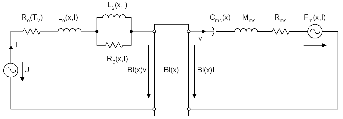
The main nonlinearities can be described by the variation of inductance, force factor, and compliance over displacement. The LSI3 can identify additional nonlinearities (not all shown here), and the thermal behavior of a transducer. You find a more detailed discussion in the reference, and additional material on our website.
Force Factor Bl(x)#
Example data used in this manual is stored in the Web Example database. If not downloaded already, get it from the latest R&D release <https://www.klippel.de/go/current-rnd-release> and open the web-based database.
See also
View Results for general information on how to download this database, open and view results in dB-Lab.
Open the Transducer Parameter Identification (LSI3, LPM, MMT, MSC, BAC, IMP) Multimedia Woofer (LPM, LSI3) and double-click the LSI3 Woofer operation to display the most important windows.
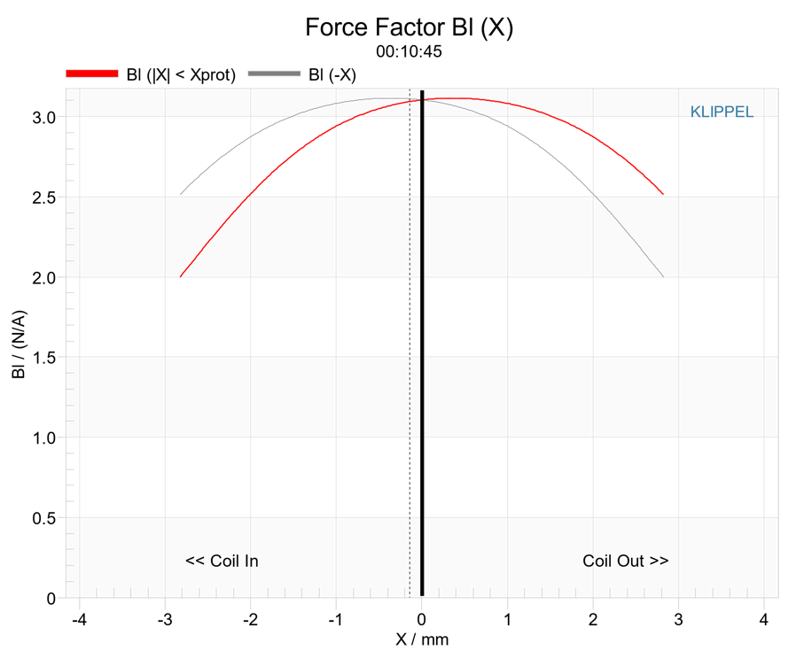
The electrodynamic coupling factor, also called Bl-product or force factor Bl(x), is defined by the integral of the magnetic flux density B over voice coil length l, and translates current into force.
In traditional modeling, this parameter is assumed to be constant. The force factor Bl(0) at the rest position corresponds with the Bl-product used in linear modeling.
The red curve displays Bl over the entire displacement range covered during the last second from actual time cursor position. You see the typical decay of Bl when the voice coil moves out of the gap. The solid gray curve displays Bl(x) mirrored at the rest position of the voice coil – this way, asymmetries can be quickly identified.
Since a laser was connected during the measurement, a vertical dashed line indicates the rest position of the voice coil at the beginning of the measurement and a “coil in / coil out” marker is displayed on the bottom left / bottom right.
Stiffness Kms(x)#
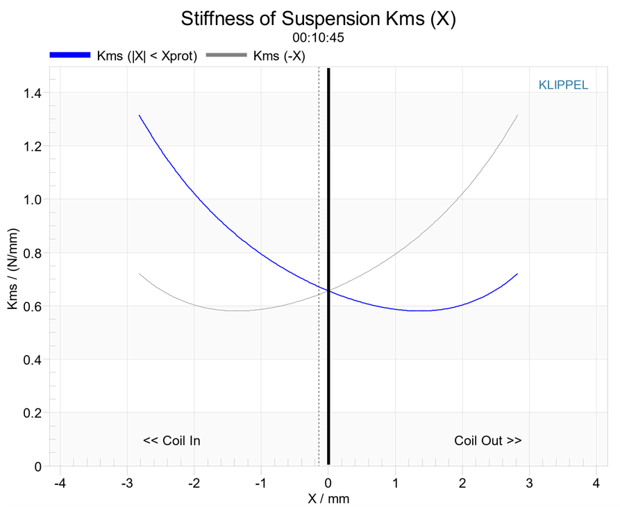
The stiffness Kms(x) describes the mechanical properties of the suspension. Its inverse, the compliance Cms(x), is also available as result window.
Inductance Le(x)#
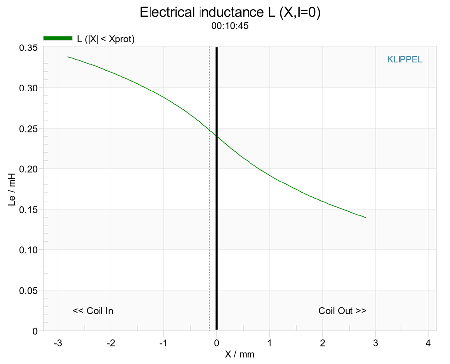
The electrical properties of the voice coil are described by the inductance Le(x), the DC resistance Re(Tv), and the para-inductance L2(x) and R2(x) that describe the effect of eddy currents in the conductive parts close to the voice coil.
The inductance Le(x) of drivers that do not comprise any shorting material has a strong asymmetric characteristic. If the voice coil moves towards the back plate the inductance increases since the magnetic field generated by the current in the voice coil has a lower magnetic resistance due to the shorter air path.
Additional Results#
Click the  Close All Windows button in the result window list, then double-click the LSI3 – Large Signal
Identification operation in the project window. This opens the default windows for the
operation - the major nonlinearities, plus the Temperature, Power result window.
Close All Windows button in the result window list, then double-click the LSI3 – Large Signal
Identification operation in the project window. This opens the default windows for the
operation - the major nonlinearities, plus the Temperature, Power result window.
Open the fS(x) result window:
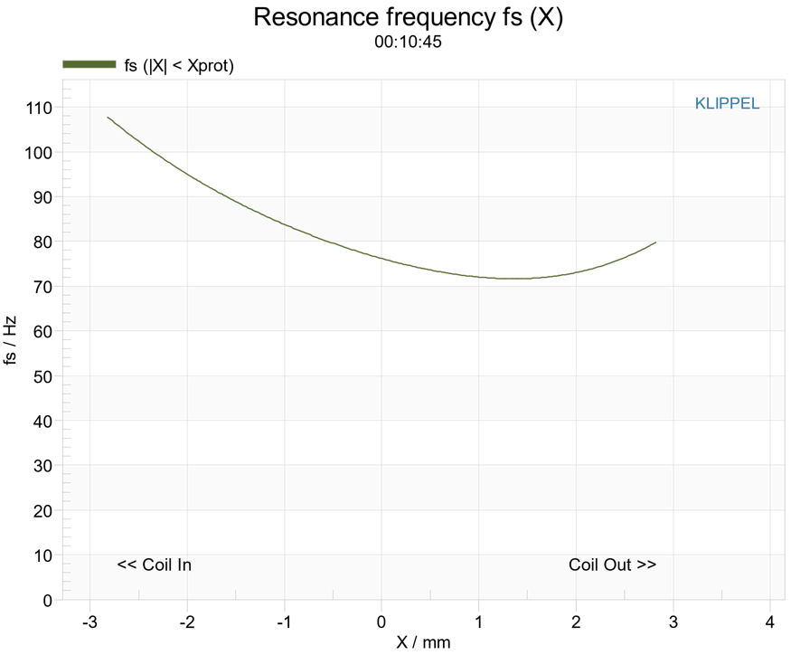
You see the increase of the resonance frequency due to increased stiffness at higher displacements.
For details of the additional results available, please refer to the reference or the specifications available from www.klippel.de
Viewing the History#
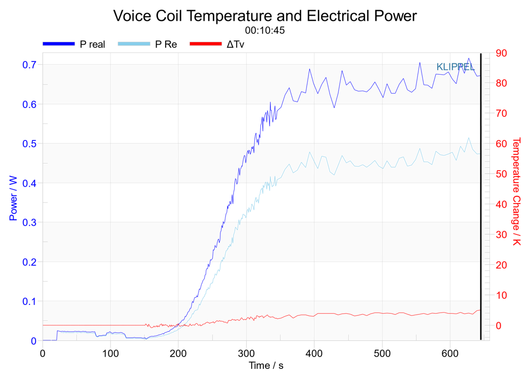
This result window shows the increase of the voice coil temperature ∆Tv and the electric input power P(t) versus measurement time, and different powers related to the thermal model.
You also see a bold black time cursor to the far right. You can drag it with the mouse, or click into the chart and move it with the Cursor left/right keys while holding down Ctrl.
When you move the time cursor around you see the other windows change their display to reflect the state of the driver at the selected time. This allows you to review the identification process, and the changes of parameters over time with increasing amplitude.
The time cursor is available in all windows where x-axis denotes the measurement time.
Nonlinear Parameters, Displacement Limits#
Open the Nonlinear Parameters result window. It contains a table with important derived nonlinear metrics describing displacement limits and asymmetries.
Part 2: Do Your First Measurement#
Setting up the Hardware#
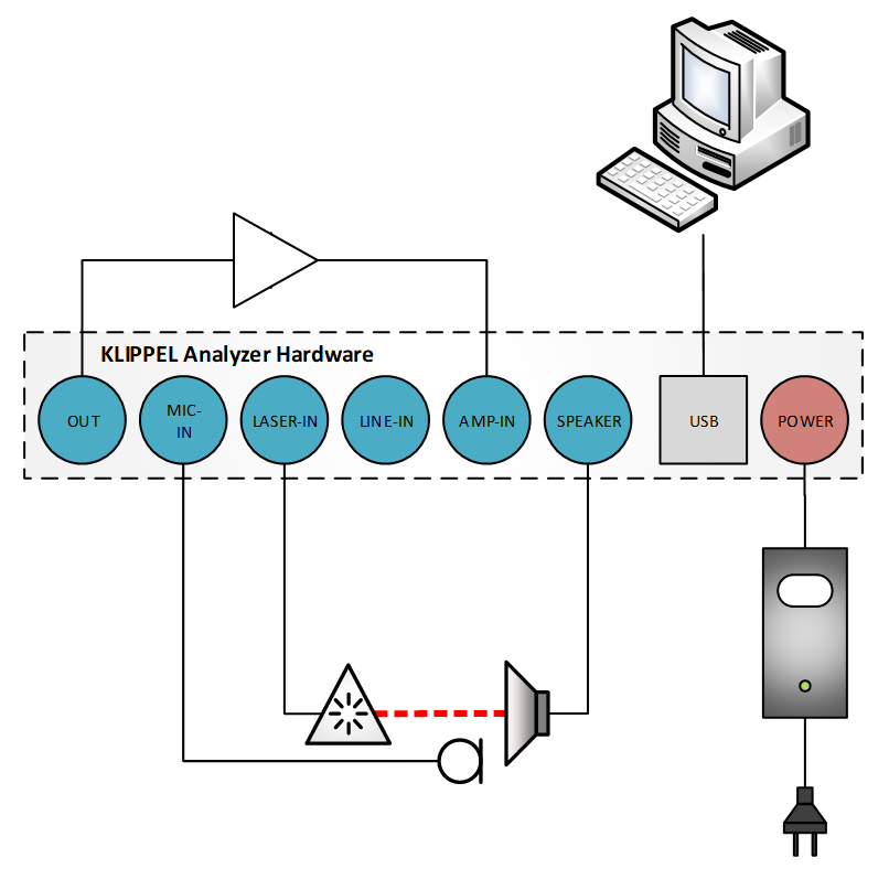
The basic hardware setup can be seen in the figure underneath. For more Information, please see the Klippel analyzer’s hardware manual
Note
The LSI3 uses a protection system that adapts well to a wide range of drivers. Before using a very small driver with a low impedance, please see Protection Parameters and How the Protection Works for adjusting protection limits and small signal gain.
Warning
Safety Information: The LSI3 can be used for destructive testing to determine the maximum limits (power, temperature, voltage, displacement) which are permissible for the drive unit. The user is responsible to comply with safety requirements. Note that overload of the driver may cause a fire hazard.
Using a Laser#
Warning
CAUTION LASER RADIATION!
See the laser sensor manual for basic information about laser measurements.
Connect the laser head via the laser controller to the hardware unit.
Make a dot of white ink (e.g. correction fluid) on the diaphragm and adjust the Laser to this point.
Ensure that the rest position of the diaphragm is in the middle of the laser’s working range.
Starting a Measurement#
Note
The LSI3 is available in two different versions (Woofer+Box and Microspeaker). You can follow this tutorial with any of these, as long as you have a licence. For more information, see LSI3 Versions.
In dB-Lab, create a new object.
Create
 a new LSI3 operation.
Double click on the LSI3 operation to open a default set of result windows. Since no measurement was performed, the charts are empty.
Make sure the hardware unit is set up correctly and connected to the PC with the USB cable.
Verify that the settings in the Protection category are appropriate for your driver
Warning
Wrong settings can damage your driver. See PROTECTION CATEGORY in the reference section for more information. Be especially careful with micro-speakers and telecommunications drivers.
Make sure that the polarity is correct. We recommend that a positive displacement represents an outward movement of the voice coil.
Click
 Run to start the measurement.
The measurement will check the amplifier, and then automatically find the working range based on the default protection parameters. For more information on the protection limits, see Part 3: Customizing the Measurement. For more information on the individual steps of the LSI, see Modes of Operation.
If a laser is connected, coil out and coil in will be displayed in the respective result windows. Note that this information relies on correct polarity of the laser calibration.
Finish Measurement#
By default, the measurement will finish automatically if the nonlinear parameters are identified.
You are able to finish by pressing the  Save/Finish button.
Note
The  Cancel Operation button changes to
Save/Finish when the most
important data is available. It is recommended to wait until the measurement has finished for best results.
Cancel Operation button changes to
Save/Finish when the most
important data is available. It is recommended to wait until the measurement has finished for best results.
Part 3: Customizing the Measurement#
Protection Parameters#
The LSI3 determines the maximum working range automatically, it uses protection parameters that are adaptive to a wide range of drivers. The default setting is safe for most drivers with 40 Hz < fs < 150 Hz, but may be overly protective especially for large ones. For very small drivers (like headphone drivers) you might need to lower the small signal gain, and/or use more restrictive settings.
Select the LSI3 operation in the project window.
Click
 View Properties, and select the Protection page, where you can change the protection settings
Available Protection Parameters are:
Increase of temperature
decay of Bl(x) and Cms(x)
real input power
Note
Smaller values for Bllim and Clim give more aggressive measurements.
If you change the protection parameters while a measurement is running, the operation will go back into the Enlargement Mode to adjust the working range based on the new settings.
Import Parameters from LPM#
The Large Signal Identification uses only electrical information (current and voltage) at the speaker’s terminals to measure the elements of the pure electrical equivalent circuit and the shape of the nonlinear curve for force factor (Bl-product), Compliance Cms and Stiffness Kms as relative quantities, e.g.:
where xprot is the allowed limit of the displacement detected by the automatic gain adjustment. Thus the relative compliance Cms,rel (xrel) is displayed in the range –1 < xrel < 1. At the rest position holds Cms,rel (x=0)=1.
The absolute identification of the mechanical parameters (e.g. Cms in mm/N) can easily be accomplished by importing at least one known parameter value (Bl(0) or Mms):
Open the DRIVER category.
Provide the parameter Bl or Mms, e.g. from the LPM – Linear Parameter Measurement Module (LPM).
The clipboard may be used for the transfer:
Open Property Page Im/Export in LPM and press Export button
Open Property Page Im/Export in LSI3, press Import button (Both parameters are imported, but only one is available at the same time)
Note
You can identify the absolute values also by using a laser. However, importing a mechanical parameter is more accurate and robust, as the LPM – Linear Parameter Measurement is more immune against measurement noise, vibration of the laser stand at high amplitudes and detects certain malfunctions of the laser (like limiting) automatically.
Modify Test Noise#
The category Stimulus allows modifying the properties of the noise used as excitation signal.
The automatic setting optimizes the signal towards best identification of the mechanical parameters, by putting all energy around the resonance frequency for high displacements and relatively low heating. For improved detection of thermal parameters and inductance characteristic, it can be beneficial to select a larger bandwidth.
How to Get the Best Performance#
Although the measurement runs almost automatically, the setup parameters accessible on the property pages may be used to optimize performance.
Import Bl(x=0)#
Although the mechanical parameters may be provided in absolute terms by using a laser, we recommend to import the Bl(x=0) via the property page IM/EXPORT. The Klippel module LPM Linear Parameter Measurement is dedicated for providing the force factor Bl at the rest position x=0 and for measuring the moving mass. After performing an LPM open the property page IM/EXPORT and press the export button. Select the new LSI3, open the property page IM/EXPORT, and press button Import from Clipboard. The Bl(x=0) may be imported at any time (before or after the measurement). Available data will always be calibrated automatically.
Optimal Noise Bandwidth#
During the parameter measurement, the internal model is fitted to the transducer by minimizing the error Ei between estimated and measured current. Typically the error Ei will become below 20 % for most drivers at the end of the Nonlinear Mode. Transducers having a high of inductance or a non-regular frequency response will cause a higher fitting error, which will degrade the accuracy of the measurement. However, by adjusting the spectral properties of the used noise signal this effect can be substantially reduced.
In the vast majority of LSI3 measurements, a change of the stimulus settings is not recommended and required, as the LSI3 is automatically finding the correct settings. The LSI3 uses the following metrics to determine the optimal bandwidth:
For woofers, the LSI3 uses a pink noise signal and a cut-off frequency of the low pass \(f_\mathrm{low} \approx 8 f_{\mathrm{s}}\) where fs is the resonance frequency of the driver.
The high-pass cut-off frequency is approx. set to \(f_\mathrm{high} < 0.5 f_\mathrm{s}\) to provide sufficient excitation below resonance.
Optimal Working Range#
The adaptive identification determines parameters giving the best fitting over the working range \(-x_{\mathrm{p}} < x < x_{\mathrm{p}}\) where the probability of the occurrence of the coil is more than 99 %. This range is about 20 % smaller than the peak displacement xprot allowed by the protection system.
For this reason, we recommend to adjust the protection parameters in such a way to measure the curves up to xprot which is 20 % higher than the peak displacement required for further analysis and system design.
Small Signal Amplitude Level#
The LSI3 measurement procedure starts in the small signal domain defined by the small signal RMS voltage Usmall. The starting amplitude is not very critical in most cases. However, if the level is very low, the measurement will take quite long.
How to Measure Micro-Loudspeakers and Tweeters#
Some tweeters and special loudspeakers intended for telecommunication have no regular suspension (spider) that can provide a mechanical protection of the voice coil. Contrary to measuring woofers, the maximum peak displacement xmax is not detectable automatically by monitoring the variation in Bl(x) and Kms(x). To protect your driver, use the maximum input power Plim to find the limits of the allowed working range.
Note
You may change the value Plim during the measurement (and the system returns into the Enlargement Mode).
It is recommended to use an appropriate laser sensor during the LSI measurement that measures the peak, bottom and mean displacement directly and shows the orientation of the x-axis (coil in and coil out position).
Those results can be compared with the predicted displacement (based on current and voltage monitoring) in the Displacement result window. The predicted displacement describes the dynamic generation of a dc component due to asymmetries in the driver nonlinearities (such as Bl(x), Kms(x), …). It cannot reflect a shift of the rest position caused by other causes such as gravity (changing from vertical to horizontal driver position), visco-elastic behavior of the suspension and static air pressure generated by heating of the air sealed below the diaphragm. The shift of the rest position during the LSI3 measurement is also displayed in the nonlinear parameter windows Bl(x), Kms(x), Le(x).
LSI3-Reference#
LSI3 Versions#
With the release of LSI3 on KLIPPEL Analyzer 3, two different versions are available:
LSI3 Woofer, identifying drivers up to fs = 400 Hz.
Apart from measuring in free air, closed or vented box systems (2nd or 4th order total mechanical-acoustical system) can be measured.LSI3 Micro-Speaker, for identifying micro-speaker drivers with fs >= 100 Hz.
The LSI3 specification provides detailed technical information about the differences. If not stated otherwise, features discussed in this manual are available for all versions. Even though the internal measurement procedures are different, we have kept the user interface as consistent as possible between the versions.
Large Signal Modeling#
At higher amplitudes, loudspeaker, headphones and other actuators produce substantial distortion in the output signal, generated by nonlinearities inherent in the transducer. The dominant nonlinear distortions are predictable and are closely related with the general principle, particular design, material properties and assembling techniques of the transducer. The Klippel Analyzer 3 combines nonlinear measurement techniques with elaborated computer simulation to explain the generation of the nonlinear distortions, to identify their physical causes and to give suggestion for constructional improvements. Better insight into the nonlinear mechanisms makes it possible to further optimize the transducer in respect of sound quality, weight, size and cost.
An electro-mechanic equivalent circuit with lumped elements can model electrodynamic transducers at low frequencies successfully. This model is characterized by Structure, free Parameters and State information. The structure of the model represents the transducer principle and the basic physical mechanisms in the transducer. The free parameters of the model vary with the transducer type and from unit to unit. Finally, the state quantities depend on initial conditions of the actuator such as ambient temperature, mounting condition, acoustic sound field and on the electric excitation signal.
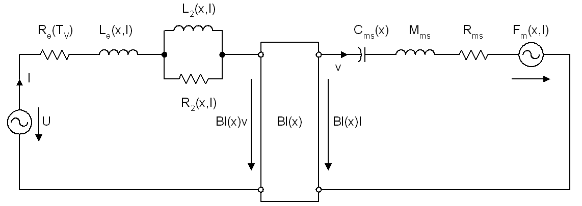
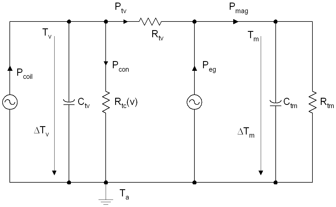
The state of the transducer can be described by using the following state variables that are time signals
- x(t)
displacement of the voice coil
- v(t)
velocity of the voice coil
- i(t)
electric input current
- u(t)
the driving voltage at loudspeaker terminals
- P(t)
real electric input power
- Tv(t)
temperature of the voice coil
- Tm(t)
temperature of the magnet structure
- \(\triangle T_{\mathrm{v}}(t) = T_{\mathrm{v}}(t) - T_{\mathrm{a}}\)
increase of voice coil temperature
- \(\triangle T_{\mathrm{m}}(t) = T_{\mathrm{m}}(t) - T_{\mathrm{a}}\)
increase of the temperature of magnet structure
- Ta
temperature of the cold transducer (ambient temperature)
- Mms
mechanical mass of driver diaphragm assembly including voice-coil and air load
- Rms
mechanical resistance of driver suspension losses
- Bl(x)
instantaneous electrodynamic coupling factor (force factor of the motor) defined by the integral of the magnetic flux density B over voice coil length l
- Re
Voice coil resistance at DC
- Cms(x,t)
mechanical compliance of driver suspension (the inverse of stiffness Kms(x,t))
- Le(x,I)
part of voice coil inductance which is independent on frequency
- Fm(x,I)
reluctance force
- L2(x)
para-inductance of the voice coil
- R2(x)
electrical resistance due to additional losses caused by eddy currents
- Pcoil
total power \(P_{\mathrm{coil}} = \ P_{\mathrm{Re}} + \alpha\cdot( P - P_{\mathrm{Re}} - P_{\mathrm{m}})\) transferred to the voice coil, defined by the power splitting factor α, the real power P supplied to the transducer, and the power PRe dissipated in resistance Re, and the mechanical power Pm transferred to the mechanical and acoustical system
- Pmech
apparent mechanical power \(P\left( t \right) = K\left( x \right) \cdot x\left( t \right)\frac{dx\left( t \right)}{dt}\) that is transferred to the suspension parts of the transducer
- Peg
power \(P_{\mathrm{eg}} = (1 - \alpha) \cdot ( P - P_{\mathrm{Re}} - P_{\mathrm{mech}})\) directly transferred to the iron via eddy currents
Some of the lumped elements have parameters that are almost independent on time and on the loudspeaker state and are used as constant parameters in congruence with linear loudspeaker theory.
The dominant nonlinearities are modeled by displacement depending parameters. The force factor Bl(x) and the inductance parameters depend on the instantaneous displacement only and are almost time-invariant as long as the rest-position of the voice coil is not changed. However, the stiffness Kms(x,t) of the mechanical suspension is also a function of the preceding displacement time signal to explain fatigue, hysteresis, creep and temporal changes.
Parameter variations caused by the voice coil excursion generate harmonic distortion and intermodulation distortion products in the frequency band the transducer is used at. Therefore, these elements have to be considered as nonlinear elements and the varying parameters are referred to as nonlinear parameters.
The electric resistance Re(Tv) of the voice coil depends on the instantaneous voice coil temperature Tv. However, the temperature Tv changes slowly and the variations of Re(Tv) do not generate additional distortion components in the audible band. Therefore, the electric resistance Re(Tv) can be modeled as a linear, time-varying element.
System Identification#
The LSI3 identifies the parameters and state information of the transducer under normal working conditions. In addition to the Thiele-Small parameters that are valid only at small amplitudes, the LSI3 additionally identifies parameters that describe the thermal and nonlinear behavior in the entire working range.
The Klippel R&D System measures the free parameters of the extended loudspeaker model in a full dynamic measurement. The loudspeaker is excited with noise (LSI3 Woofer) or a multi-tone stimulus (LSI3 Micro-speaker). Optimal parameters are estimated by nonlinear system identification based on adaptive inverse control, using the voltage and current signals that are available at the loudspeaker terminals.
The system generates a test signal and monitors the instantaneous states and the parameters of the loudspeaker. The detailed data is collected in a protocol and is transferred via the USB interface to a computer for further inspection. During all modes of operation, the measurement system provides the permanent information about the progress and the results of the system identification. A protection system can be activated to keep the peak displacement and voice-coil temperature below a defined threshold (e.g. to protect a unique prototype).
The expanded transducer model with identified parameters is the basis for numerical simulations to predict the nonlinear and thermal behavior of the transducer in different applications (SIM2, SIM‑AUR modules). Harmonic and intermodulation distortion components can be calculated for any multi-tone excitation signal and compared with measured responses. Simulation of the nonlinear behavior is less time-consuming than the direct measurement and allows an analysis of the loudspeaker’s nonlinearities. The contribution of each nonlinearity to the total distortion can be calculated and thus the source for the dominant distortions can be detected.
This information is crucial for finding the weakest point in the loudspeaker design and to give some indications for constructional improvements. Some of the nonlinearities can be reduced without increasing the cost of the speaker. Asymmetries in the parameter characteristics can be detected and second-order distortion can be reduced by an optimal adjustment of the voice-coil and the mechanical suspension.
Measurement Condition#
It is recommended to measure the loudspeaker driver in free air with the loudspeaker axis pointing in horizontal direction to prevent gravity from acting on the moving mass. A special loudspeaker stand simplifies the mounting and gives easy access for a Laser Displacement Sensor. The standard baffle as specified in IEC 60268-5 is also a convenient method of loudspeaker mounting.
Transducers should be measured under conditions such that the mechanical system including any acoustical load can be represented as a second- or fourth-order system. To measure the parameters of a driver (woofer, tweeter, micro-speaker, exciter, shaker, headphone …) at highest precision it is recommended to operate the driver in free air. Measuring a woofer in free air also requires less electrical input power, and produces less noise, than measuring the same driver in a closed system. LSI3 Woofer measures the driver parameters of a fourth-order system such as a vented or passive radiator system.
A special stand proved to be useful to clamp woofers in a vertical position and to measure the displacement of the diaphragm by a Laser displacement meter is also available as dedicated accessory by Klippel. Because there is no additional microphone needed, the acoustic environment in greater distance has a minor influence on the loudspeaker parameters so the measurement can also be performed in a normal working room or in a power test room.
Excitation Signal#
The KLIPPEL Analyzer 3 needs an excitation signal with sufficient amplitude and spectral properties to identify the transducer completely. A single sinusoidal signal with constant frequency and amplitude would allow identifying a system with two free parameters only. Clearly a multi-tone signal at high frequencies or a flute concert without any bass content would not generate high excursions of the voice coil producing nonlinear distortion components, which are the basis for detecting the transducer’s nonlinearities. Most of ordinary audio signals such as full orchestra music or pop music give persistent excitation but require a signal source (CD-player). However, an artificial noise signal used for simulating program material as specified in IEC 60268-1 is preferable and more convenient for transducer measurements. This signal can easily be generated in a DSP with desired properties in respect of spectral properties and reasonable amplitude distribution and enables the system identification to find the optimal parameters in a short time.
DC Resistance Limits#
The voice coil resistance limit depends on the selected Speaker Channel sensitivity. To change
the sensitivity for a selected channel, open the KA3 Signal Configuration  and set the
sensitivity to the desired value.
and set the
sensitivity to the desired value.
The current limits are
Low Sensitivity: 0.5 Ω \(\leq R_{\mathrm{e}} \leq\) 100 Ω
High Sensitivity: 1 Ω \(\leq R_{\mathrm{e}} \leq\) 1000 Ω
Modes of Operation#
The measurement procedure is organized in initial identification, and long-term monitoring and additional modes of operation.
Step |
Modes of Operation |
Comment |
|---|---|---|
1/2 |
Amplifier Mode |
Amplifier check without transducer excitation |
3 |
Linear Mode |
Measurement of the linear parameters in the small signal domain |
4 |
Enlargement Mode |
Identification of the allowed working range (xprot, Pmax) |
5 |
Nonlinear Mode |
Identification of the nonlinear parameters |
Exception Mode |
Malfunction explained by error message |
The current mode is displayed in the result State window.
Amplifier Mode 1 (Step 1)#
Determines the time delay of the amplifier.
Amplifier Mode 2 (Step 2)#
Before driving the loudspeaker with the excitation signal the additional equipment (power amplifier, cables, clamps) are checked in respect of
connectivity
gain of the amplifier
polarity (180 degree phase shift) of the signal
nonlinear distortion produced by the amplifier
linear transfer function (phase and amplitude response)
If the amplifier check is not successful, the Klippel Analyzer enters the Exception Mode where the measurement is aborted and a malfunction message is issued.
Linear Mode (Step 3)#
After performing the Re-measurement, the loudspeaker is excited with a small amplitude signal. Since the variations of the nonlinear parameters and the heating of the voice coil can be neglected, the identified parameters correspond with the results of a traditional small-signal measurement. The voice coil resistance related to the ambient temperature \(T_{\mathrm{v}} = T_{\mathrm{a}}\) measured in this step is used as a reference to estimate the increase of voice coil temperature \(\triangle T_{\mathrm{v}} = T_{\mathrm{v}} - T_{\mathrm{a}}\) in the following measurements.
Enlargement Mode (Step 4)#
After convergence of the linear parameter estimation, the thermal and nonlinear parameters are estimated in the large signal domain by increasing slowly the amplitude of the excitation signal until one of the protection criteria reaches the predefined limit values and the maximum range of safe operation is detected. The Enlargement Mode uses the fastest possible learning speed.
Nonlinear Mode (Step 5)#
After finding the optimal range of operation, the convergence of the nonlinear parameters at high amplitudes requires some time (5 min) because the occurrence of displacement peaks is relatively rare. The learning speed is reduced.
Exception Mode#
The measurement of the large-signal parameters is aborted if a malfunction is detected. In any case, the state of the controller is frozen and the Klippel Analyzer automatically disconnects the loudspeaker from the amplifier output. An error message is displayed on the graphical user interface.
The Klippel Analyzer checks all the other adaptive parameters and indicates a malfunction of the system identification (Exception Mode) if the values are beyond a physically meaningful range and disconnects the transducer from the power amplifier.
How the Protection Works#
The Enlargement Mode is a very critical mode because the limits of the working range have to be identified safely. An overload situation can be detected by monitoring the thermal, mechanical and electrical state quantities and the variation of the nonlinear parameters. Electrodynamic transducers may be destroyed by thermal and mechanical overload initiated by the electric signal at the terminals.
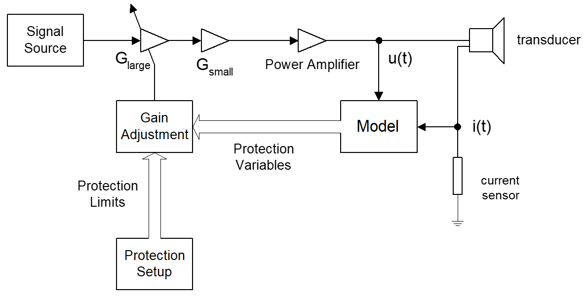
Thermal Load#
The heating of the loudspeaker is a relatively slow process that can be easily checked by monitoring the increase of the voice coil temperature ∆Tv(t). If the voice coil temperature exceeds an allowed limit value, the amplitude of the excitation signal has to be reduced to prevent from damaging the assembly. It should be noted that ∆Tv(t) describes the mean temperature of the voice coil averaged over all windings. Usually, windings close to the pole piece and pole plate have a lower temperature than windings outside the gap. These differences in local temperature might become substantial in transducers with a long voice coil overhang.
Mechanical Load#
The voice coil displacement x(t) is a quantity which can describe the load put on the mechanical system. If the displacement exceeds an allowed peak value xmax the diaphragm, parts of mechanical suspension (spider, surround) or even the voice coil former may be endangered to permanent destruction. Thus, the maximum displacement xmax is a very important parameter in the specification of the transducer related to the maximum acoustic output at low frequencies.
However, the displacement x is not as convenient as a protection variable if the maximum displacement xmax has not yet been specified for the particular driver. Therefore, a quantity is required which directly describes the geometrical changes of the suspension that indicate an overload situation. The nonlinear characteristic of the compliance reflects this information and the minimal compliance ratio Cmin summarizes this in a convenient one-value parameter. Following usual transducer design the mechanical capability is limited by the spider or at least by the surround. Such transducers can handle a variation of Cmin down to 20 % without any damage. The measured Cmin also reflects other limiting mechanisms, e.g. the voice coil former hitting the back plate. However, hard limiting occurs at a distinct amplitude without any warning and cannot be anticipated from Cmin at lower amplitudes.
The maximum variation of the force factor Blmin is another useful criterion to detect the maximum displacement xmax of the voice coil. This parameter reflects the ratio of the voice coil height to the thickness of the pole plates in the motor structure. A maximum force factor variation Blmin < 50% produces substantial distortion components in the output signal spreading over the whole transfer band of the transducer and shows the end of the useable working range.
Note
The working range of tweeters, headphones, micro-speakers and other transducers without spider is usually not limited by a progressive Cms-nonlinearity. Here the input power Plim might be used to operate the transducer in the permissible working range and avoid a destruction of the coil due to hard limiting.
Amplitude#
Usmall represents the small signal excitation RMS-value at the beginning of the measurement, where the transducer can be operated safely. Its allowed range is 0.125V \(\leq U_{\mathrm{small}} \leq\) 5V. This value should usually be higher than the voltage used for a small signal measurement (LPM). The DUT should behave sufficiently linear without heating up the voice coil at Usmall. If Usmall is too low, the measurement will take unnecessarily long In the Enlargement Mode, the amplitude of the excitation signal is increased until a protection limit ∆Tv, Blmin, Cmin or Plim is reached.
The measurement of micro-speakers and headphones requires a relatively low amplifier gain (< 10 dB between input and output). Make sure that the gain is sufficient if larger drivers are measured. The maximum achievable peak output voltage umax can be checked in Table States. Note that this value represents the maximum voltage that the analyzer can deliver with the gain of the connected amplifier. The amplifier might clip at much lower values already.
Note
Before dB-Lab version 212.228, the large signal gain Glarge was limited to 26 dB. In newer dB-Lab releases the available gain is higher. Check the available headroom of the analyzer’s output signal Lheadroom in Table States.
Protection Limits#
For each protection variable a parameter describing the allowed limit value is specified on the section Protection on the SETUP property page:
- ∆Tlim
allowed increase of voice coil temperature ∆Tv,
- Bllim
allowed minimal value of the force factor ratio Blmin,
- Clim
allowed minimal value of the mechanical compliance ratio Cmin,
- Plim
allowed maximum value of electric input power P.
Default Protection Parameters#
The limit parameters ∆Tlim, Bllim and Clim can be considered as general setup parameters. Setting these to conservative values ∆Tlim =90 K, Bllim =50 % and Clim =50 % where the protection of the driver is the main concern, these setup parameters are suited for a wide range of transducers. To test a speaker at the thermal limits some technical details about the voice coil, the glue used and the material of the former are required. The maximum electric input power Plim can be used as a more restrictive protection parameter, which is independent on the identification of the thermal and nonlinear mechanisms.
Aggressive Measurements#
You can manually increase the protection parameters before or while the operation is running. If you notice any problems such as voice coil rubbing or the voice coil former hitting the back plate, you should set more conservative protection parameters immediately.
Property Pages#
Property Pages and Setup-Categories#
Select the LSI operation in the project window, and click the  “View properties”
button. The property pages contain setup parameters, control the display of the results and allow user
interaction with the identification process running in the Klippel Analyzer. Certain parameters can be
adjusted even when the measurement is already running.
“View properties”
button. The property pages contain setup parameters, control the display of the results and allow user
interaction with the identification process running in the Klippel Analyzer. Certain parameters can be
adjusted even when the measurement is already running.
The following sections give a short summary of the Property Pages and Setup Categories:
INFO Page#
The Info page allows the user to change the name of the measurement and to add a comment to the measurement.
SETUP Page#
- Driver
The Driver category contains special transducer parameters which can be provided by the user.
- Stimulus
The Stimulus category gives access to setup parameters of the noise generator.
- Routing
The Routing category contains the routing configuration, e.g. used Speaker-Card input as well as output channel.
- Measurement Setup
The Measurement setup category allows specifying the mode at which the measurement will be finished.
- Protection
The Protection page gives access to the parameters used for controlling the amplitude of the excitation signal.
- Processing
The Processing category allows changing several post-processing parameters, such as virtually switching the driver polarity or the thresholds for the displacement limits.
IM/EXPORT Page#
The Im/Export Page allows the user to import known small signal parameters (Bl(0), Mms, Re) from other measurements (LPM Linear Parameter Measurement).
DRIVER Category#
The Driver category contains special transducer parameters, which have to be provided by the user.
- Enclosure
- Range: Free air, Sealed, Vented
Select whether the driver is operated in free air, in a sealed or vented enclosure.
- Air Volume Vb
- Air Volume Vb in literRange: 0.001 \(< V_{\mathrm{b}} <\) 10000
Specifies the air volume of the box if sealed or vented enclosure is selected.
- Bl(x=0)
- Bl(x=0) in N/ARange: 0 \(< Bl(x = 0) <\) 100
Force factor at the rest position of the voice coil.
- Mms
- Mms in gRange: 0 \(<M_{\mathrm{ms}} <\) 1000
Moving mass of driver diaphragm assembly including voice-coil and air load.
- Re(ΔTv=0 K)
- Re(ΔTv=0 K) in OhmRange: 0
Voice coil resistance at DC
- Diaphragm Area SD
- Diaphragm Area SD in cm2
The diaphragm area is the effective projected surface area of the driver diaphragm.
- Diameter dd
- Diameter dd in cm
Alternatively insert the diameter of circular diaphragm. The diaphragm area Sd will be calculated.
- Nominal Impedance Zn
- Nominal Impedance Zn in Ohm
The electrical impedance rated by the manufacturer.
- Material of Voice Coil
- Range: Copper, Aluminum, Custom
The kind of material used for the voice coil has to be specified if known. This information is used to identify the increase of voice coil temperature from the variations of the voice coil resistance.
If a Laser Displacement Sensor is not available or the signal-to-noise-ratio of the sensor output is poor, the mechanical quantities cannot be identified as absolute values but can only be presented as relative parameters. Using the Im/Export-page, the user may import the force factor Bl(0) at the rest position and/or the mechanical mass of driver diaphragm assembly including voice-coil and air load Mms. By specifying one of those values, relative parameters and states are transformed into absolute values based on physical units.
Please note that an entry on this category has a higher priority than the laser measurement. Thus, all entries have to be cleared to use the Displacement Sensor for identification of the mechanical system.
Re(ΔTv=0K) import#
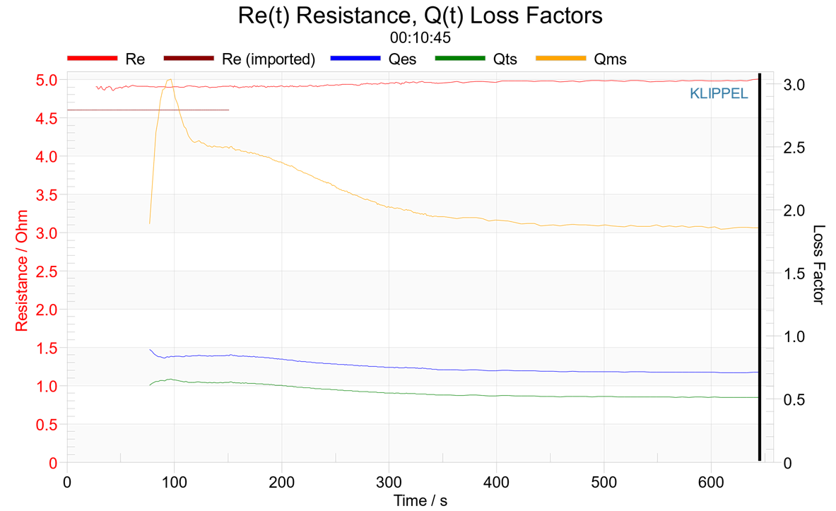
The imported Re value will be drawn as solid line up to the end of the Linear Mode in the Re(t) and Qes(t) result window. It allows to compare the Re that was measured by the LSI3 with the imported Re.
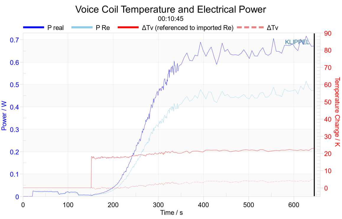
A higher Re measured by the LSI3 is typically caused by a preheated voice coil due to previous measurements or using a too high excitation voltage during the Linear Mode. If the imported Re is activated, the Delta Tv result curve represented by a dashed line in the Temperature and Electrical Power result window shows the temperature increase during the measurement. This value will also be used for the thermal protection. A 2nd Delta Tv (referenced) result curve represents the total temperature increase from referenced ambient conditions.
It must be guaranteed that the LPM measurement results used for the LSI3 import have been done at referenced ambient conditions.
STIMULUS Category#
The Stimulus category gives access to setup parameters of the noise generator.
- Urms max
- Urms max in V
Approximated maximum achievable RMS voltage during transducer identification. (read only)
- Usmall
- Usmall in VRange: 0.125 \(\leq U_{\mathrm{small}} \leq\) 5
The small signal excitation voltage can be used to select the optimal signal amplitude in the Linear Mode, where the transducer can be operated safely.
- Automatic
The band-pass filter will be adjusted to the particular driver automatically. In the Linear Mode the cuit-off frequency of the high-pass \(f_{\mathrm{hp}} = 0.5 f_{\mathrm{s}}\) and the cut-off frequency of the low-pass \(f_{\mathrm{lp}} = 8 f_{\mathrm{s}}\) will be adjusted according to the resonance frequency fs.
- Spectral Characteristic
- Range: Pink, White
Random noise (LSI3 Woofer) or a multi-tone signal (LSI3 Microspeaker) with a pink or white spectral characteristic may be generated. Additional bandpass filtering and amplitude compression may be supplied.
- Boost Resonance
If checked, applies a signal boost around the identified system resonance frequency for higher power efficiency. This reduces voice coil heating during the measurement.
- Shaping
- Range: Relative Cut-off Frequency, Cut‑off Frequency
Type of noise shaping 2nd order bandpass filter. Depending on this option, you can either choose absolute or relative cut-off frequencies for the filter.
- Highpass cutoff frequency fhp
- Highpass cutoff frequency fhp in HzRange: 10 – 150
A high pass of second order will be applied to the white or pink signal.
- Lowpass cutoff flp
- Lowpass cutoff flp in HzRange: 100 – 1500
A lowpass of second order will be applied to the white or pink signal.
- Highpass fhp/fs
- Highpass fhp/fs in HzRange: 0.1 – 1
A high pass of second order will be applied to the white or pink signal.
- Lowpass flp/fs
- Lowpass flp/fs in HzRange: 1 – 20
A lowpass of second order will be applied to the white or pink signal.
ROUTING Category#
The Routing category gives access to routing of the measurement device used for the identification.
- Speaker-Card Channel
- Range: 1, 2
Used channel of the Speaker Card for the measurement. You can change the current sensitivity in the KA3 Signal Configuration.
- Apply stimulus at
- Range: Out1, Out2
Output channel used for the measurement.
MEASUREMENT SETUP Category#
The Measurement Setup category allows modifying the conditions under which the transducer is measured.
- Finish after
- Range: Automatic; Linear Mode; Enlargement Mode; Nonlinear Mode
The measurement procedure will finish the measurement after processing the mode specified by the user. For a description about the modes, see Modes of Operation. Choose Automatic to stop the measurement after the last mode supported by the current LSI3 version.
- Duration of ‘Nonlinear Mode’
- Duration of ‘Nonlinear Mode’ in minRange: 0 – 60 min
The user can specify the duration of the Nonlinear Mode to ensure an optimal convergence of the parameters. Loudspeakers with a high voice coil overhang require a longer measurement time than drivers with an equal-length configuration.
PROTECTION Category#
The Protection category gives access to the parameters used for controlling the amplitude of the excitation signal. During the measurement, the parameters in this category can be modified. To find the working range, the LSI3 increases the drive voltage until one state approaches its limit.
If a measurement is started, the current state of the protection parameters is displayed behind the name in parenthesis.
Warning
Wrong settings can damage your driver. See Setting Protection Parameters below.
- ∆Tlim
- ∆Tlim in KelvinRange: 0 \(< \triangle T_{\mathrm{v}} <\) 300
allowed increase of voice coil temperature ∆Tv as defined by the user in the protection property page (also used as a target value for thermal identification)
- Bllim
- Bllim in %Range: 25 % \(< Bl_{\mathrm{lim}} <\) 100 %
allowed minimal value of the force factor variation ratio Blmin as defined by the user in the protection property page
- Clim
- Clim in %Range: 20 % \(< C_{\mathrm{lim}} <\) 100 %
allowed minimal value of the mechanical compliance ratio Cmin as defined by the user in the protection property page
- Plim
- Plim in WRange: 0 \(< P_{\mathrm{lim}} <\) 1000 W
allowed maximum value of electric input power P as defined by the user in the protection property page
Setting Protection Parameters#
Choosing the correct settings is crucial to protect your driver, and lets you define how “aggressive” the measurement is. Here are some practical tips which settings are relevant – but always remember that your driver may be different. Be especially careful for tweeter and telecommunication drivers!
The protection system will not detect all causes of failure, like tearing wires or the voice coil hitting the back plate. Always keep an eye on unknown driver types and your expensive prototypes.
Temperature: Remember that ∆Tlim specifies a temperature increase relative to the beginning of the measurement. Let thermally sensitive drivers cool down before you repeat a measurement.
Also, the temperature is an average over the voice coil length. Portions of the coil may be much hotter.
Mechanical Protection: (Bllim and Clim): These are often the limiting factors for subwoofers and midrange drivers, and they are suited for driver sizes over a wide range, from subwoofers to midrange drivers. Thus, the default settings work usually very well for these drivers.
However, they often do not provide protection for tweeters and micro-speakers.
Power Plim: For tweeter measurements, it is best to start with a low power, and increase it during the measurement, as described below
Changing Protection Parameters during Measurement#
When you measure a type of driver for the first time, we recommend starting with strong protection parameters (low Power and ∆T, high Bllim, Clim). Monitor the driver for clicking and other unusual noise and unstable behavior.
In the Protection category you can see which parameter is limiting, and if more excitation is suitable. When you change the limiting protection parameter(s), the measurement will go back into the Enlargement Mode and adjust the excitation level to the new limits. You can repeat this until you have found the excitation level you are confident with.
PROCESSING Category#
The Processing category allows to change post-processing parameters, such as virtually switching the driver polarity or defining displacement limits.
- Switch Polarity
If checked, the driver polarity is virtually switched in post-processing. This allows you to cope with wrong polarity without physically changing the drivers connectors
- Displacement limits
Specifies if the displacement limits are calculated using the IEC 60268 or with custom settings.
- Blmin
Force factor decay allowed at XBl.
The Protection Parameter Bllim should be up to ca 20 % lower than Blmin.- Cmin
Compliance decay allowed at XC.
The Protection Parameter Clim should be up to ca 20 % lower than Cmin.- Zmax
Maximum variation of Inductance allowed at XL.
- d
Maximum Doppler distortions allowed at XD.
IM/EXPORT Page#
- Import from Clipboard
You may import Bl(x=0), Mms and Re(∆Tv=0) from the clipboard which are used setup parameters. Note that if you import setup parameters, all results of the LSI3 operation are deleted.
- Export to Clipboard
Press this button to copy all setup parameters and large signal parameters to the clipboard. You may view the results within the clipboard by using the editor provided by dB-Lab. The clipboard data can e.g. be used to export linear and nonlinear parameters into a simulation tool, such as the SIM Simulation module module.
All modules supporting LSI3 import and export functionality are documented in chapter Supported Modules for Im/Export.
Reconnect to Klippel Analyzer 3#
In the unlikely event that you have to attach to a running measurement, you can attach to a measurement using the following steps:
In the dB-Lab project window, select the LSI operation that you disconnected from
Click the
 Run button.
The Device selection dialog will indicate that an LSI measurement is still running, and that you can reconnect to the running measurement. Click OK to confirm this.
Results#
The results of the measurement consist of state and parameter information. The state information describes the physical quantities of the transducer and the signals related with the system identification in the last update interval. This data depends on the instantaneous properties of the excitation signal. The parameter information refers to the transducer and shows a minor dependence on the excitation signal. However, the parameter estimates are not constant but show some stochastic fluctuations due to the measurement noise and some systematic changes due to reversible and non-reversible mechanisms (heating, aging, creep).
Parameters#
In contrast to linear loudspeaker theory the large signal modeling considers that loudspeaker parameters depend on instantaneous loudspeaker state variables. Thus, important loudspeaker parameters such as Bl-factor, compliance and inductance are not assumed as constant but depend on the instantaneous displacement x of the voice coil. Other parameters such as mechanical damping might be also considered as variables but contribute less to the nonlinear behavior of loudspeakers at high amplitudes.
- \(-x_{\mathrm{prot}} < x < x_{\mathrm{prot}}\)
The maximum displacement range detected by the automatic gain adjustment (limited by the protection system). The current parameter estimates of the nonlinear elements are displayed as a function of the displacement in this range.
- \(x_{\mathrm{bottom}} < x < x_{\mathrm{peak}}\)
During the measurement, a black line indicates the peak and bottom value \(x_{\mathrm{bottom}} < x < x_{\mathrm{peak}}\) that occurred in the last update interval.
- Relative parameters and displacement
If the mechanical parameters are represented as relative quantities (e.g. Kms(x) / Kms(0), Bl(x) / Bl(0), …) and the displacement is expressed as x / xprot, then the mechanical system has not been identified in absolute terms. Please use a laser or import the parameters Bl(0) and/or Mms via the IM/EXPORT property page.
- Orientation of the displacement
The user may change the sign of the displacement by changing the polarity of the SPEAKER cables (blue and red) connected to the driver’s terminals. A negative displacement should represent a movement of the coil towards the back plate. Please refer to the marks coil in and coil out for the current orientation of displacement.
- Coil In / Coil Out
When a laser sensor is used durig the the LSI3 measurement, the marks coil in and coil out are shown at the bottom of the diagrams depending on diplacement. The coil in mark should always represent a movement of the voice coil towards the back plate.
Force Factor Bl(x)#
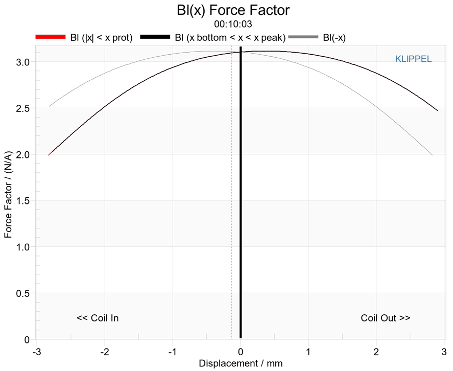
The electrodynamic coupling factor, also called Bl-product or force factor Bl(x), is defined by the integral of the magnetic flux density B over voice coil length l. In traditional modeling this parameter is assumed as constant. The force factor Bl(0) at the rest position corresponds with the Bl-product used in linear modeling.
During the measurement, the black line indicates the current working range (peak and bottom displacement) in the last update interval.
The solid gray curve Bl(-x) indicates the force factor mirrored at the rest position. This helps to identify asymmetries related to the y-axis of the chart. The solid black vertical line represents the instantaneous rest position of the voice coil (if the stimulus would be switched off). The instantaneous rest position should be used for coil alignment.
Note
Displaying the rest position requires a laser sensor and a reliable signal during the measurement (displacement error <= 5 %). Do not move the sensor during LSI measurement.
Stiffness Kms(x)#
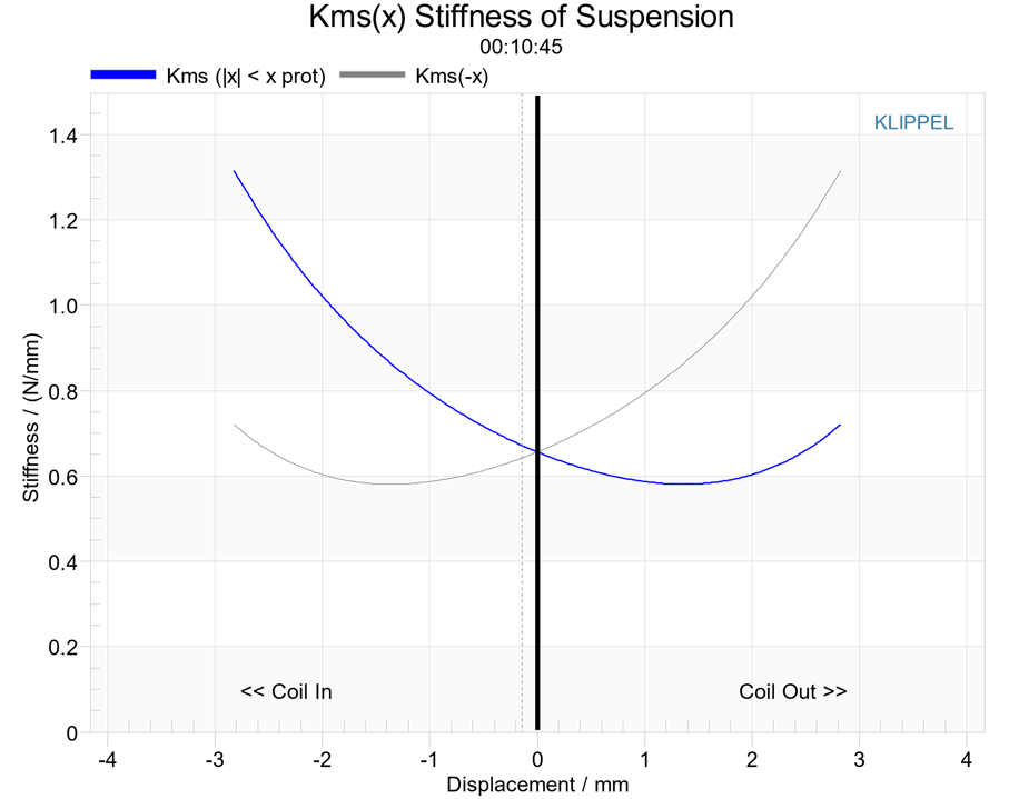
The stiffness Kms(x) describes the mechanical properties of the mechanical suspension and is the inverse of the compliance Cms(x).
For a description of the different curves, see “Force Factor Bl(x)”.
- LSI with Box-Enclosure
If an enclosure was chosen, the chart will also display the total stiffness of the entire system Kmt(x) as dotted line. For the driver compliance to be displayed, both Sd and the box volume Vb at section Driver on property page SECTION needs to be set correctly.
Note that you can change Sd and Vb after the measurement is complete. However, enclosure type must be set before the measurement.
Compliance Cms(x)#
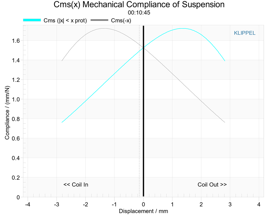
The compliance Cms(x) is the inverse of the mechanical stiffness.
Inductance Le(x)#
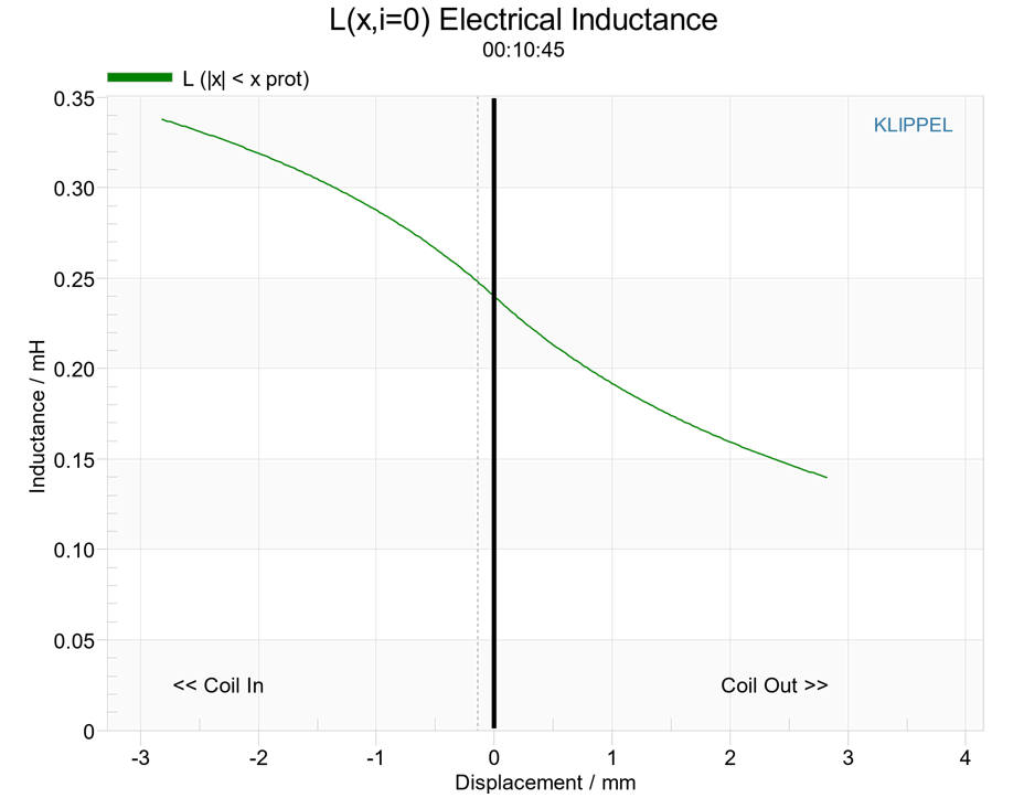
The electrical properties of the voice coil are described by the parameters Re(Tv), Le(x), L2(x) and R2(x). The last three parameters are required to describe the effect of eddy currents in the conductive parts close to the voice coil.
The inductance Le (x) of most drivers has a strong asymmetric characteristic. If the voice coil moves towards the back plate, the inductance usually increases since the magnetic field generated by the current in the voice coil has a lower magnetic resistance due to the shorter air path. This property can be used for checking the polarity of the loudspeaker and to interpret the direction of the excursion in the diagrams of the nonlinear parameters.
Inductance Le(i)#
(LSI3 Woofer only)
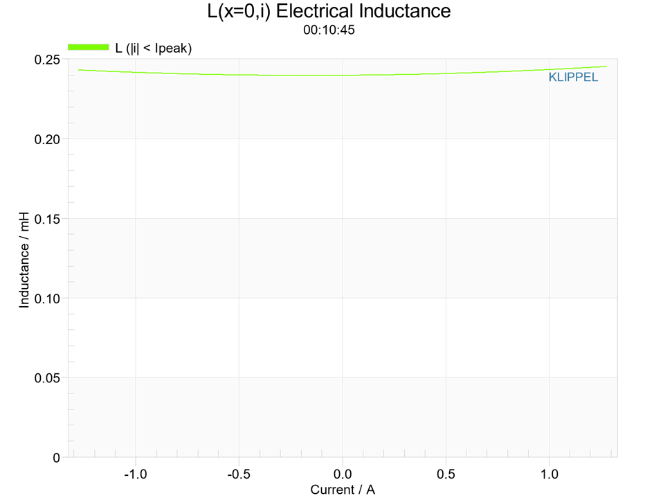
For woofers, the variation of the inductance Le versus voice coil current is measured. This kind of nonlinearity is closely related with variation of the permeability of the iron in the pole plates and piece. Le(i) varies only little if the iron is highly saturated by the static flux generated by the permanent magnet. Le(i) contributes to the harmonic distortion measured at frequencies above resonance frequency fs.
Mechanical Resistance Rms(v)#
(LSI3 Micro-speaker only)
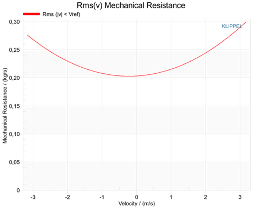
The dependency of the mechanical resistance Rms on voice coil velocity v is a dominant nonlinearity in micro-speakers and other transducers which have a relatively high resonance frequency fs, a relatively small force factor Bl and a total quality factor Qts dominated by the mechanical losses. This nonlinearity can be neglected in woofers using a strong motor with a high value of the force factor Bl, a small dc resistance Re and being operated by a voltage supply where the electrical damping dominates the mechanical damping.
The nonlinear variation of Rms-nonlinearity is not caused by the mechanical vibration of the diaphragm or other mechanical elements, but by the nonlinear air flow resistance in the tiny structures (usually the transducer’s motor). Measurements show that the nonlinearity vanishes when the micro-speaker is operated in vacuum. For details, see W. Klippel, Modeling the Large Signal Behavior of Micro-speakers.
The Rms(v) nonlinearity causes a significant increase of mechanical damping at resonance frequency, causing a nonlinear amplitude compression of the fundamental and generating significant harmonic and intermodulation distortion.
Resonance Frequency fs(x)#
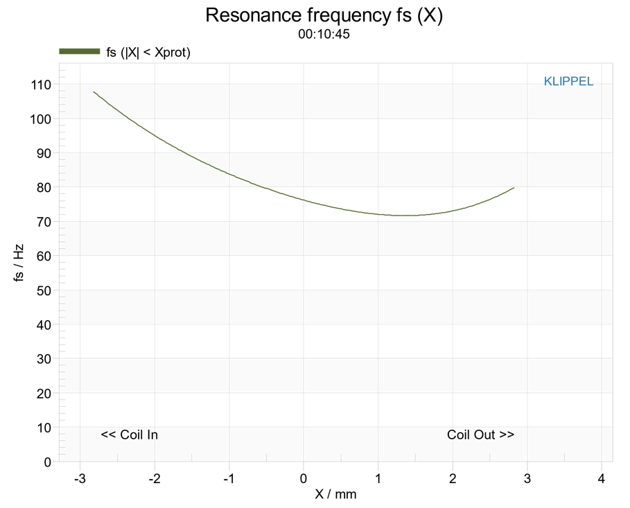
The instantaneous resonance frequency fs(x) is displayed as a function of voice coil displacement x caused by the variations of the mechanical compliance defined by
Total Loss Factor Qts(x)#
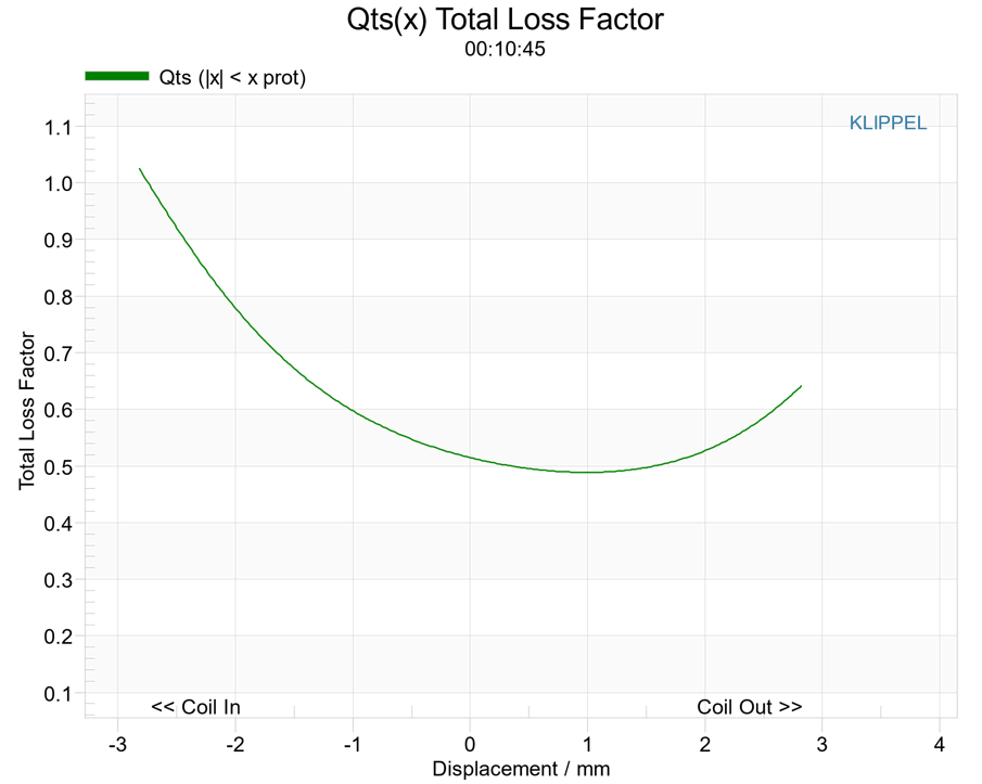
The total loss factor Qts(Tv, x) defined as
summarizes the effect of mechanical and electrical damping. In a voltage driven woofer connected to a low impedance source, the electrical loss factor Qes(x) usually dominates the total loss factor Qts (x) at small amplitudes. The mechanical loss factor might become dominant at higher amplitudes if the force factor Bl(x) varies substantially with the displacement.
Impedance Z(f)#
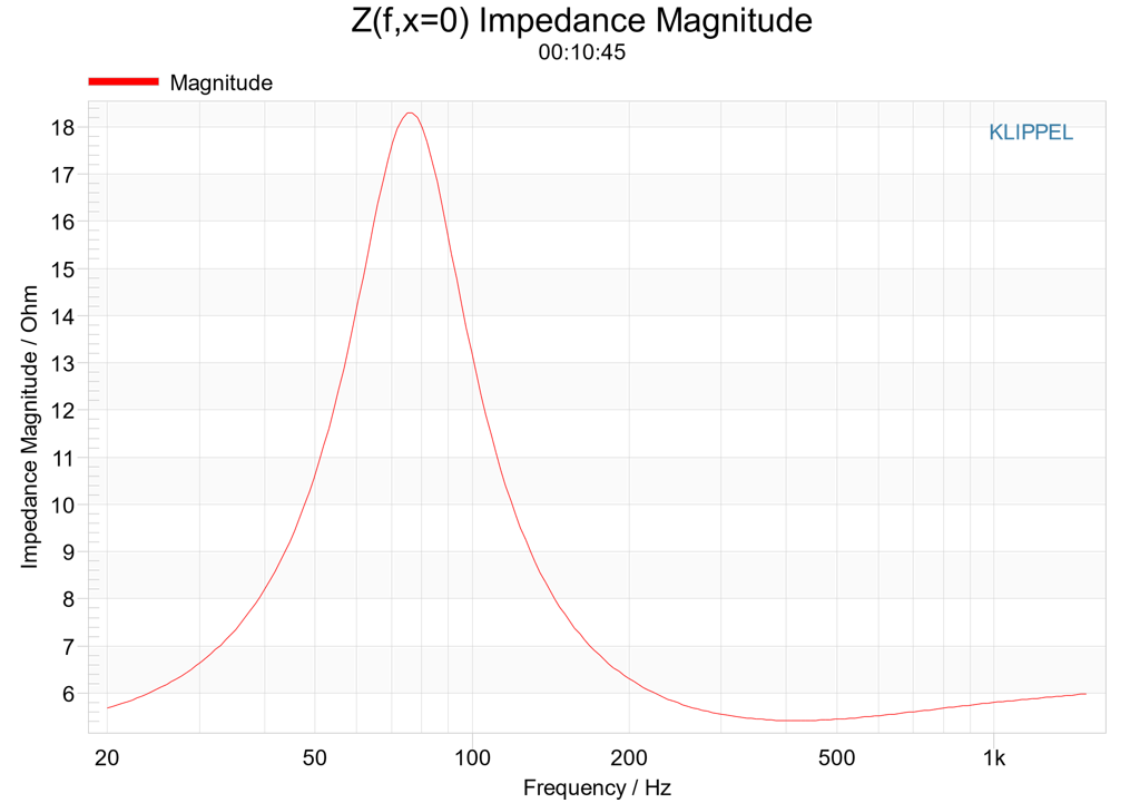
The electrical impedance Z(f) of an electro-dynamic transducer in free air is
It represents the ratio between terminal voltage U(f) and current I(f). The curve is derived from the estimated small signal parameters as shown in the Large + Warm column in the window Table Parameters at x=0.
Nonlinear Parameters#
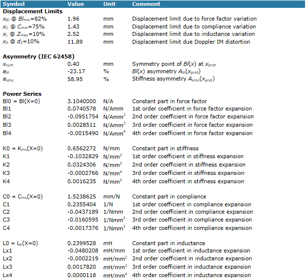
This table shows the parameter-based displacement limits xBl, xC, xL and xD. The default thresholds of these limits are set according to IEC 60268. They can be modified in the Processing section in the Setup property page.
Displacement Limit xBl#
The maximum displacement xBl limited by excessive motor distortion can be obtained from the nonlinear force factor characteristic Bl(x). We define the minimal force factor ratio
which is the ratio of the minimal force factor Bl(x) in the working range ±XBl referred to the Bl-value at the rest position x = 0. XBl is implicit in the equation and can be found in the nonlinear Bl(x)-characteristic after defining the threshold Blmin.
Displacement Limit xC#
The maximum displacement related to the critical mechanical strain of suspension may be obtained from the nonlinear stiffness characteristic Kms(x) or from its counterpart, the compliance characteristic Cms(x). Introducing a minimal compliance ratio
which is the ratio of the minimal value of the compliance within the working range ±xC and the value at the rest position x = 0.
xC is implicit in the equation and can be found in the nonlinear Cms(x)-characteristic by using a pre-defined threshold Cmin.
Displacement Limit xL#
The complicated frequency characteristic of the voice coil inductance is caused by the para-inductance of the coil and additional losses due to eddy currents. This can be modeled by a lumped parameter model comprising the electrical DC resistance Re, the voice coil resistance Le(x) and the additional elements L2(x) and R2(x) in parallel. For the nonlinear elements we assume the same shape of the curve giving
The variation of the impedance versus displacement x is directly related with the magnitude of the intermodulation distortion generated in the current and in the radiated sound pressure output. Thus, the displacement limit xL is defined implicitly by
which is the ratio of the maximum variation of the electrical impedance at frequency f2 within the working range \(-x_{\mathrm{L}} < x < x_{\mathrm{L}}\) and the impedance at the rest position x = 0.
To keep the parameter-based method consistent with the performance-based method, the frequency \(f_{2} = 8.5 f_{\mathrm{s}}\) is coupled to the resonance frequency fs and the impedance can be approximated by
with \(s_{2} = 2 \pi f_{2} j\) .
Displacement Limit xD due to Doppler#
The peak displacement xD considering the audibility of the Doppler Effect can be calculated analytically using the simple equation
presented by Beers and Belar [33], using the peak displacement xpeak in mm, the second-order modulation distortion d2 in percent according to IEC 60268 and the frequency f2 of the modulated voice tone. To keep the definition of xD consistent with the performance based method we set \(f_{2} = 8.5 f_{\mathrm{s}}\) and use the distortion threshold d = 10 %, giving a Doppler displacement limit
where xD is in mm and fs is in Hz.
Coefficients of the Power Series#
The nonlinear force factor
compliance of the driver suspension
stiffness of driver suspension
inductance versus displacement
and inductance versus current
are expanded in a power series expansion where x is the voice coil displacement in mm, i is the voice coil current in A and the nonlinear coefficients are given by the result window Table Nonlinear Parameters.
Parameters at x = 0#
Note
For the most accurate small signal parameters, use the LPM Linear Parameter Measurement module.
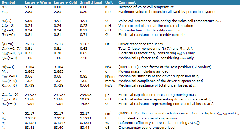
The values of the nonlinear parameters at the rest position (x = 0) are of special interest for the linear approximation of the driver behavior. The values of the parameters at the rest position (x = 0) can be used as input parameters for a linear modeling.
However, the time-variant parameters Cms(x=0,t), Kms(x=0,t) and Re(Tv) usually differ from the corresponding small signal parameters due to heating, creep and aging.
Using the history information of the parameters sampled during measurement time, the result window Table States gives the parameter at the rest position for three different modes of operation.
LARGE+WARM (large signal domain + warm speaker)
the peak value of the displacement is high (xpeak <= xprot),
the variation of the parameters is not negligible (Cmin << 100 % and/or Blmin << 100 % and/or Lmin << 100 %),
the voice coil temperature is increased (∆Tv > 0) due to heating.
LARGE+COLD (large signal domain + cold speaker)
the peak value of the displacement is high (|x| < xprot),
the variation of the parameters is not negligible (Cmin << 100 % and/or Blmin <<100 % and/or Lmin << 100 %),
the effect of heating is compensated while considering the cold voice coil resistance measured in the Linear Mode of the initial identification where (∆Tv = 0).
SMALL SIGNAL (small signal domain + cold speaker)
the amplitude of the excitation signal is sufficiently small,
the displacement is small in comparison to the allowed maximum displacement (|x| << xprot),
the variations of the nonlinear parameters are negligible (Cmin ≈ 100 %, Blmin ≈ 100 %, Lmin ≈ 100 %),
the increase of voice coil temperature is negligible (∆Tv ≈ 0),
the effects of the nonlinear, thermal and time-varying mechanisms are negligible and the transducer behaves almost linear.
Equivalent Volume#
The volume of air having same acoustic compliance as driver suspension is
\[V_{\mathrm{as}}\left( x \right) = \rho_{0}c^{2} \cdot S_{\mathrm{d}}^{2} \cdot C_{\mathrm{ms}}\left( x \right)\]with the density of air ρ0 = 1.18 kg/m3, the velocity of sound in air c = 345 m/s and effective projected surface area of driver diaphragm Sd.
Reference Efficiency#
For a loudspeaker driver mounted in an infinite baffle the efficiency of the electro acoustical conversion with radiation into the half-space is
\[\eta_{\mathrm{0}}\left( x,T_{\mathrm{v}} \right) = \frac{\rho_{0}}{2\pi \cdot c} \cdot \frac{{b\left( x \right)}^{2} \cdot S_{\mathrm{d}}^{2}}{R_{\mathrm{e}}\left( T_{\mathrm{v}} \right) \cdot M_{\mathrm{ms}}}\]
Relationship to Linear Modeling#
The so-called Linear Parameters are required as the input parameters for traditional linear modeling. All of the parameters are assumed to be constant. The dependence on the state quantities (displacement x and temperature Tv) is neglected. In case the parameters depend on displacement, the rest position (x = 0) is used as linear parameter. This approximation is valid in the small-signal domain only. At higher amplitudes there are systematic discrepancies between small-signal and large-signal parameters due to heating and the time variance of some transducer parameters.
The traditional loudspeaker design is based on a linear modeling comprising constant parameters only. This model is simple and explains the linear transfer behavior (e.g. amplitude and phase response) at low amplitudes. The linear model can be considered as an approximation of the expanded model valid in the small signal domain. The parameters of both models are closely related with each other. However, to explain the differences we have to distinguish between small signal parameters and large signal parameters at the rest position.
Small Signal Parameters#
For measuring the small signal parameters of a linear model,
the displacement is small in comparison to the allowed maximum displacement (|x| << xprot),
the variations of the nonlinear parameters are negligible (Cmin ≈ 100 %, Blmin ≈ 100 %, Lmin ≈ 100 %),
the increase of voice coil temperature is negligible (∆Tv ≈ 0).
Under these conditions, the varying parameters of the extended model correspond with the constant parameters used in traditional modeling:
- Bl(x=0) = Bl
Force factor,
- Cms(x=0, t) = Cms
Mechanical compliance of driver suspension,
- Kms(x=0, t) = Kms
Mechanical stiffness of driver suspension,
- Le(x=0) = Le
Part of voice coil inductance which is independent on frequency,
- L2(x=0) = L2
Para-inductance of the voice coil,
- R2(x) = R2
Electric resistance due to additional losses caused by eddy currents,
- Re(TV≈TA) = Re
Electric resistance of the voice coil at ambient temperature.
State Variables#
The system identification used in the Klippel Analyzer 3 provides not only the free parameters of the transducer model but also state variables depending on the excitation signal. There are three kinds of state variables:
Transducer States
The electrical, mechanical and thermal quantities such as displacement x, velocity v, current i, power P, voice coil and magnet temperature are represented by digital variables in the DSP. These states are subject to statistical investigations and their properties can be described by peak values, rms values or other measures.
Signal Properties
The properties of the excitation signal are represented by statistical measures (peak and rms value, …)
Errors in the adaptive Modeling
The fitting of the model is described by error metrics in %.
State#
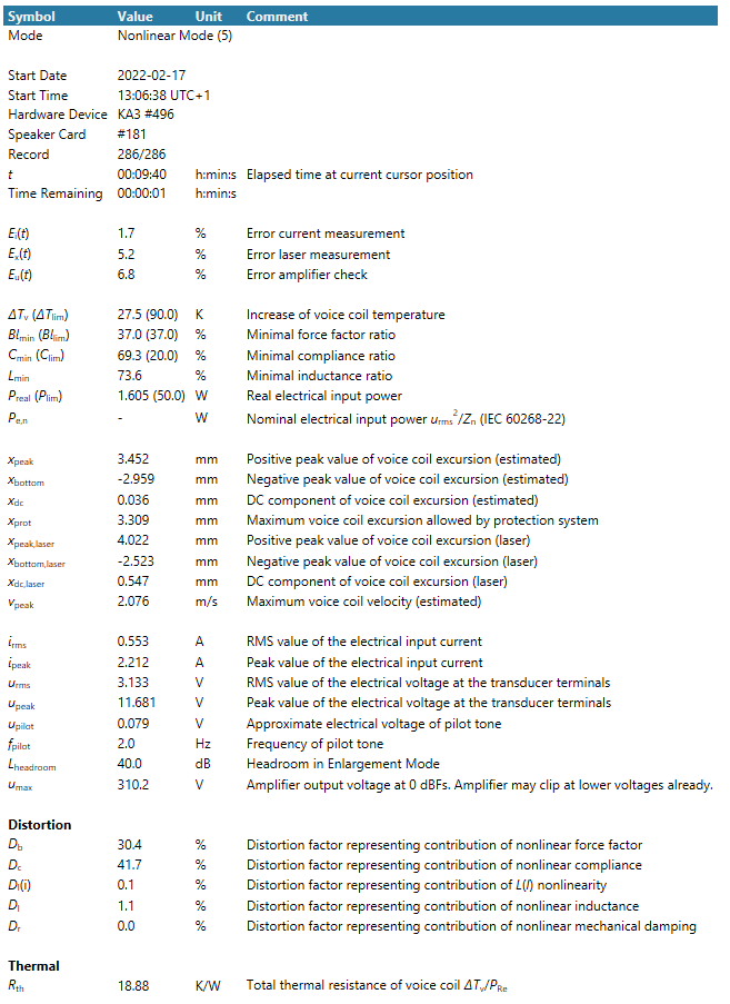
The state window gives a summary of relevant state variables at a selected time depending on the cursor position. Each entry is described in greater detail in the respective windows.
Temporal Variations of States and Parameters#
The instantaneous state variables and parameters estimated by the system identification are permanently sampled and stored in the used database. The following parameters can be displayed versus measurement time:
Voltage and Current#
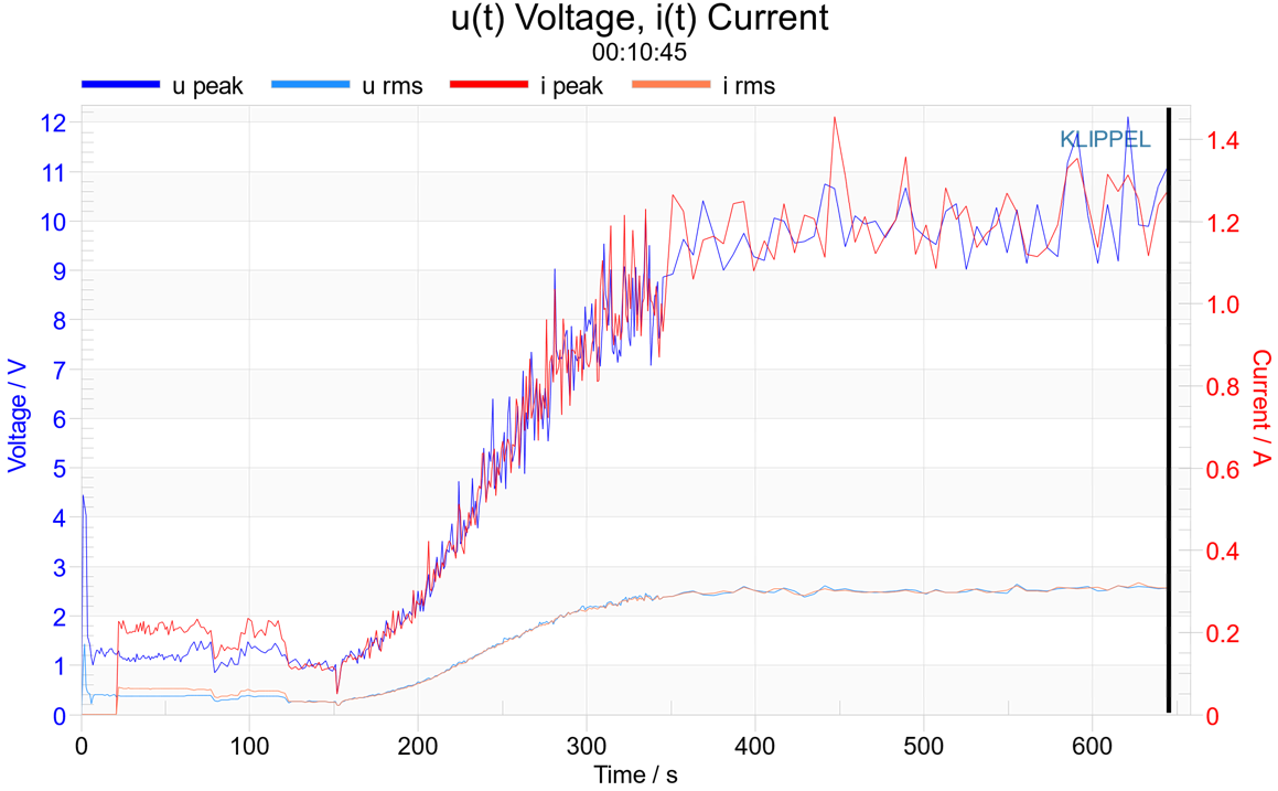
This result window characterizes the properties of the electric signals at the transducer terminals.
- urms
rms value of the electric terminal voltage
- upeak
peak value of the electric terminal voltage
- irms
rms value of the electric input current
- ipeak
peak value of the electric input current
The time cursor can be dragged with the mouse or moved to go back in measurement history.
Temperature and Electrical Power#
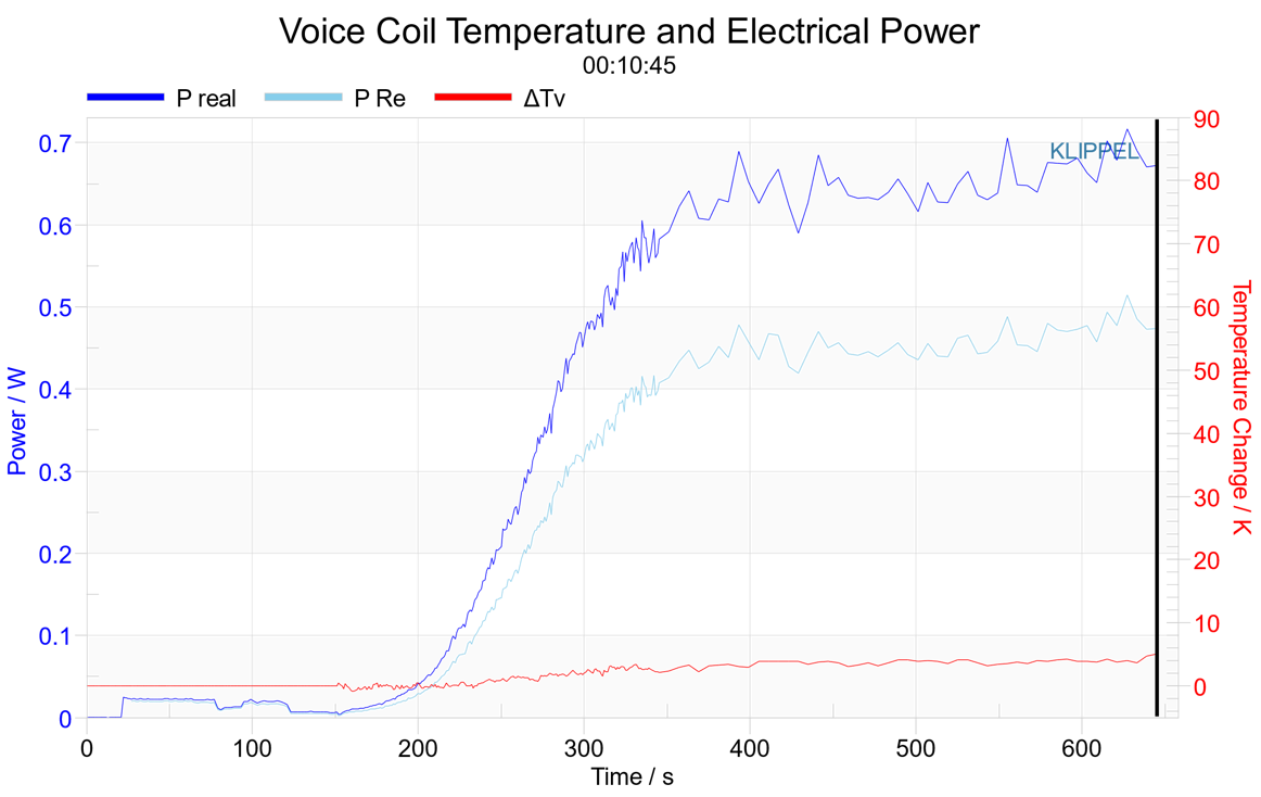
This result window shows the increase of the voice coil temperature ∆Tv and the electric input power P(t) versus measurement time.
Note that the ΔTv curve can be recalibrated. This shifts the curve so that the temperature is calculated based on this Re(Tv=0) K) value. A second curve shows the temperature that is based on the measured Re(Tv=0 K) of the LSI3’s Linear Mode.
Using this import can for instance be helpful to correct the absolute temperature if the LSI3 was started with a warm voice coil.
The different modes of operation can easily be identified in the time plot. At the beginning of the measurement where power and temperature is low, the LSI3 performs the Linear Mode and the transducer is operated in the small signal domain. The temperature of the voice coil at the end of this phase is used as reference temperature Ta that equals the ambient temperature. The increase of the input power indicates that the Enlargement Mode which identifies the allowed range of safe operation is active. Both state signals are used as protection variables and are compared with the limit values Plim and Tlim defined by the user.
PRe indicates the power that is dissipated in the voice coil.
Note
The voice coil temperature measured by the electrical impedance is an averaged value. For coils with large overhang the partial temperature at the coil ends is usually much higher than in the middle part where the conduction to the pole tips is better.
The time cursor can be dragged with the mouse or moved to go back in measurement history.
Equivalent Input Distortion Components#
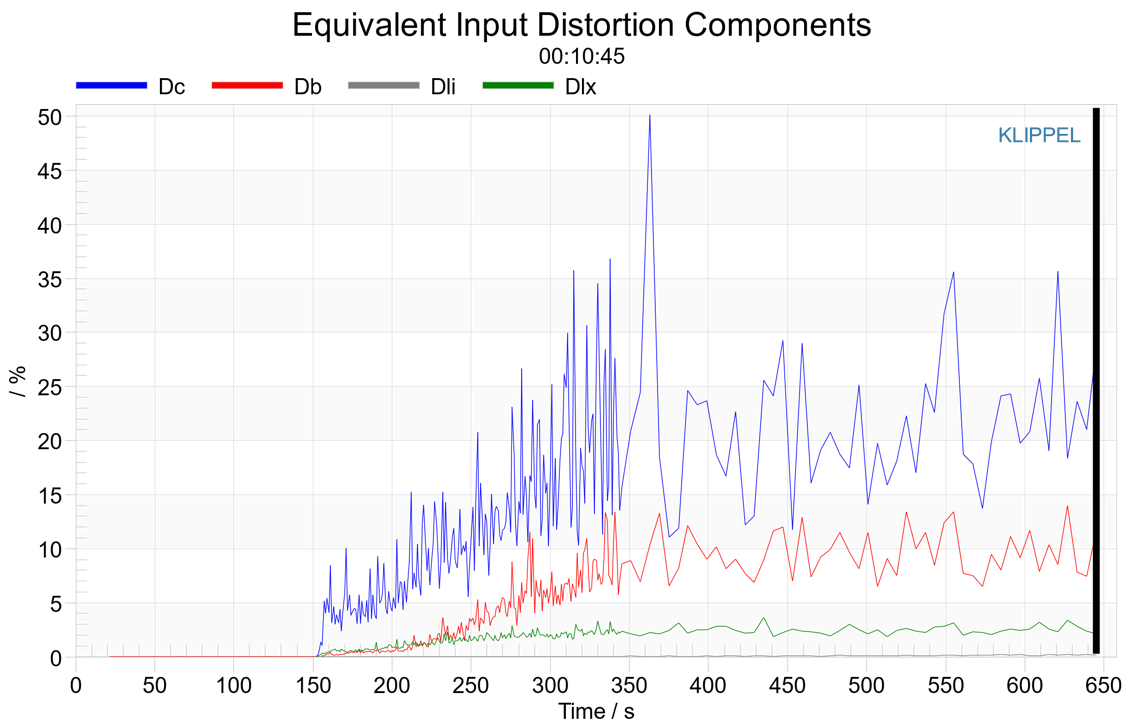
This result window shows the results of the distortion analysis performed during the measurement:
- Db
Relative equivalent input distortion representing the contribution of nonlinear force factor,
- Dlx
Relative equivalent input distortion representing the contribution of nonlinear inductance varying with displacement
- Dc
Relative equivalent input distortion representing the contribution of nonlinear compliance.
- Dli
Relative equivalent input distortion representing the contribution of nonlinear inductance varying with current (LSI3 Woofer)
- Dr
Relative equivalent input distortion representing the contribution of nonlinear mechanical resistance Rms(v)
The relative distortion factors describe the ratio of the peak values of the equivalent input distortion generated by the nonlinearity and the peak value of the total signal.
The distortion analysis shows the dominant nonlinearity producing the largest amount of signal distortion. The influence of the spectral properties of the excitation signal on the distortion can be investigated by changing the upper cut-off frequency of the excitation signal in the Stimulus category on theproperty page.
The identified model gives also access to the nonlinear distortion generated within the transducer. The simplified signal flow-chart below shows that the nonlinear mechanisms can be separated from a linear system. The signals pb(x)(t), pL(x)(t) and pC(x)(t) representing the nonlinear distortion from the nonlinear force factor Bl(x), inductance parameters Le(x), L2(x), R2(x) and the compliance Cms(x), respectively, are added to the linear signal plin(t) and are part of a feedback loop. This structure corresponds with the nonlinear differential equation implemented in real time in the DSP. In contrast to the real physical system, we can directly measure the properties of each distortion component while reproducing any excitation signal such as noise, music or a multi-tone signal.
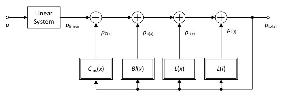
Setting the maximum peak value of the distortion signals in relation to the peak value of the total signal we can calculate the relative degree of force factor distortion
\(d_{\mathrm{b}}\left( t_{1} \right) = \frac{\max\limits_{t_{1} < t < t_{1} + \mathrm{\Delta}t}\left| p_{\mathrm{b}\left( x \right)}\left( t \right) \right|}{\max\limits_{t_{1} < t < t_{1} + \mathrm{\Delta}t}\left| p_{\mathrm{total}}\left( t \right) \right|}\),
compliance distortion
\(d_{\mathrm{c}}\left( t_{1} \right) = \frac{\max\limits_{t_{1} < t < t_{1} + \mathrm{\Delta}t}\left| p_{\mathrm{c}\left( x \right)}\left( t \right) \right|}{\max\limits_{t_{1} < t < t_{1} + \mathrm{\Delta}t}\left| p_{\mathrm{total}}\left( t \right) \right|}\),
inductance distortion (versus x)
\(d_{L\left( x \right)}\left( t_{1} \right) = \frac{\max\limits_{t_{1} < t < t_{1} + \mathrm{\Delta}t}\left| p_{L\left( x \right)}\left( t \right) \right|}{\max\limits_{t_{1} < t < t_{1} + \mathrm{\Delta}t}\left| p_{\mathrm{total}}\left( t \right) \right|}\),
and inductance distortion (versus i)
\(d_{L\left( i \right)}\left( t_{1} \right) = \frac{\max\limits_{t_{1} < t < t_{1} + \mathrm{\Delta}t}\left| p_{L\left( i \right)}\left( t \right) \right|}{\max\limits_{t_{1} < t < t_{1} + \mathrm{\Delta}t}\left| p_{\mathrm{total}}\left( t \right) \right|}\)
for every update instant t1.
The time cursor can be dragged with the mouse or moved to go back in measurement history.
Displacement#
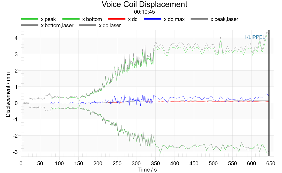
This result window shows the following statistical characteristics of the voice coil displacement versus measurement time:
- x peak
positive peak of the voice coil displacement in the update interval (predicted by using the identified model)
- x dc
averaged DC-value in voice coil excursion (predicted)
- x bottom
negative peak value (bottom value) of the voice coil displacement in the updated interval (predicted)
- x dc,max
maximum DC-value in voice coil excursion \(x_{\mathrm{DC max}}(t) = \frac{x_{\mathrm{peak}}(t) + x_{\mathrm{bottom}}(t)}{2}\)
- x min,laser
negative peak of the voice coil displacement in the update interval measured by laser displacement sensor
- x max,laser
positive peak of the voice coil displacement in the update interval measured by laser displacement sensor
- x min,laser
averaged DC-value of the voice coil displacement in the update interval measured by laser displacement sensor
Asymmetrical nonlinearities produce not only second- and higher-order distortion but also a DC part in the displacement by rectifying low frequency components.
For an asymmetric stiffness characteristic, the DC component moves the voice coil in the direction of the stiffness minimum.
For an asymmetric force factor characteristic, the DC component depends on the frequency of the excitation signal. A sinusoidal tone below with (f < fs) would move the voice coil in the direction of the force factor maximum that provides some self-adjustment of the voice coil position. However, a tone above the resonance frequency (f > fs) would generate a DC component in the opposite direction, which causes unstable behavior, loss of efficiency and nonlinear distortion.
Maximum Displacement xmax#
If the voice coil displacement x exceeds an allowed limit value xmax, the transducer generates nonlinear distortion which cannot be tolerated in the particular application or may cause a damage. The following criteria determine the definition of xmax:
prevention of suspension damage,
prevention of damage of the voice coil former by hitting the back plate,
limitation of frequency modulation distortion produced by the sound radiation (Doppler effect),
limitation by nonlinear distortion caused by parameter variations,
limitation by the ability of the voice coil to dissipate heat
Error (t)#
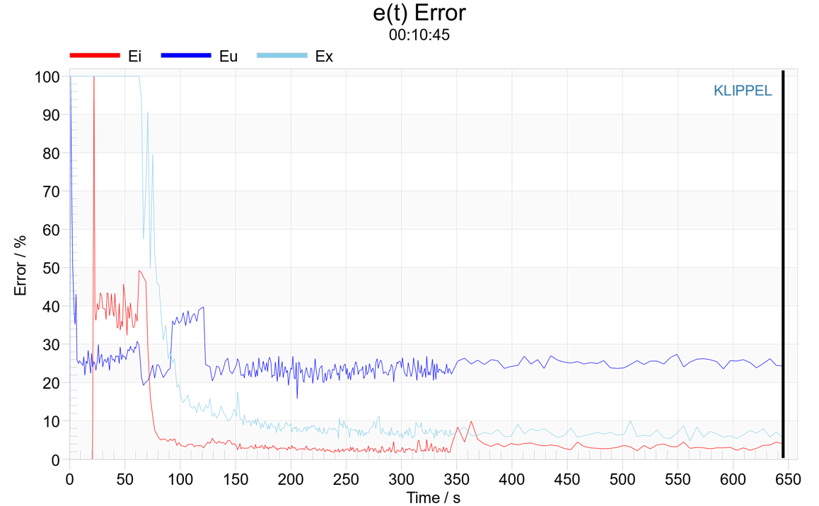
The identification process is evaluated by the following error measures:
- Ei(t)
Peak value of the relative error used in the system identification based on current monitoring by calculating the ratio of the peak value of the current error ei(t) to the peak value of the current i(t) measured during the last update interval.
- Ex(t)
Peak value of the relative error used in the system identification based on laser measurement by calculating the ratio of the peak value of the displacement error ex(t) to the peak value of the displacement x(t) measured during the last update interval,
- Eu(t)
Peak value of the relative error used in the system identification of the power amplifier by calculating the ratio of the peak value of the voltage error eu(t) to the peak value of the voltage u(t) measured during the last update interval.
At the beginning of the measurement where all free parameters of the model are set to initial values the errors Ei(t), Ex(t) and Eu(t) are about 100 % going down during the identification process.
The time cursor can be dragged with the mouse or moved to go back in measurement history.
Voltage Error Eu#
Transducers in normal operation mode are usually driven by a low impedance source and the electric voltage at the speaker terminals can be considered as an input signal. This signal deviates from the generator output if an AC-coupled audio power amplifier is used or if the amplifier starts to limit. Therefore, the system identification also detects the transfer function of the amplifier to ensure that the amplifier works properly.
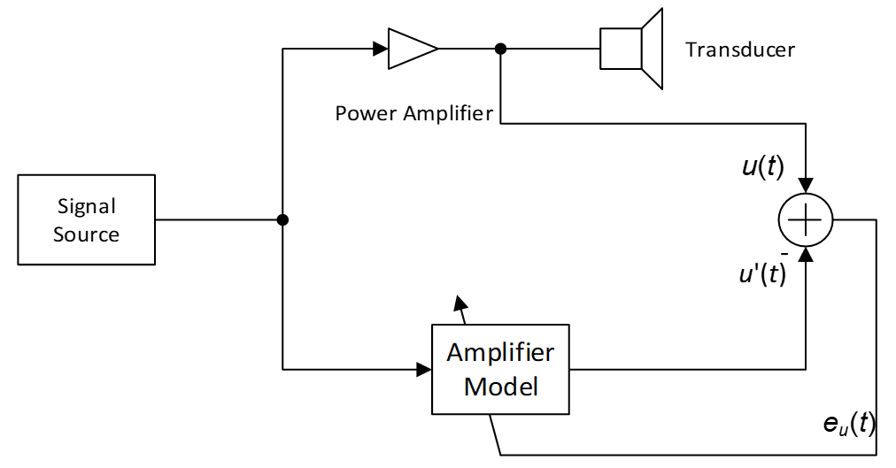
Thus, the Klippel Analyzer has an amplifier model which is adapted to the real power amplifier by minimizing the error signal \(e_{\mathrm{u}}(t) = u(t) - u'(t)\) which is the difference between the measured voltage u(t) and the estimated voltage u’(t).
The fitting of the amplifier model is described by the relative amplifier error
which is the ratio between the peak value of the error signal eu(t) and the measured voltage u(t) over the last update interval. Unidentified variations in the phase and amplitude response, nonlinear distortion and measurement noise contribute to this error measure.
Current Error Ei#
The system identification based on current measurement is illustrated in the signal flow chart below. Both the transducer and the model are provided with an excitation signal. The difference between measured current i(t) and estimated current i’(t) is used as error signal \(e_{\mathrm{i}}(t) = i(t) - i'(t)\) for the adjustment of the free model parameters.
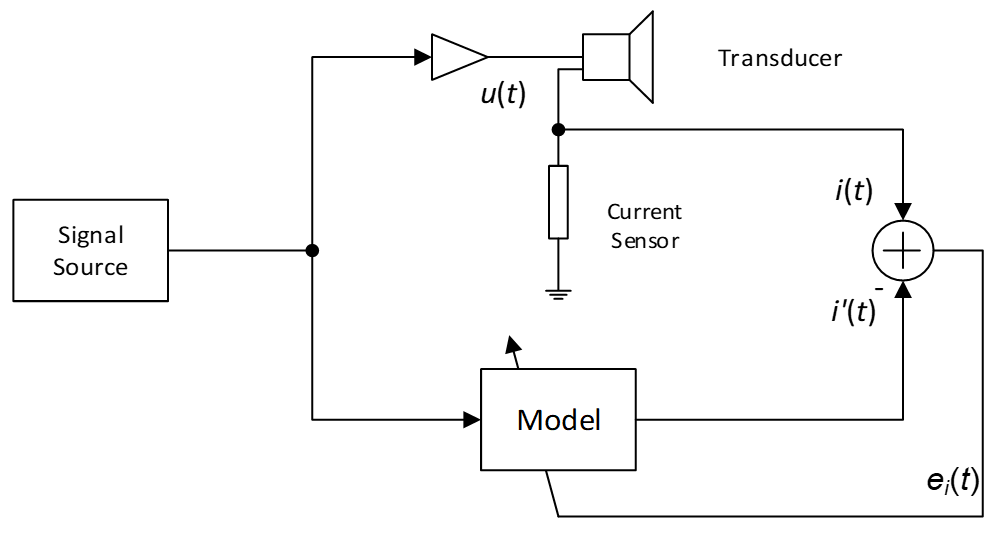
The model is optimally adjusted to the particular transducer if the magnitude of the error becomes minimal. The Klippel Analyzer 3 solves this optimization problem by using an adaptive scheme as described in [22]. In this approach the transducer model is implemented in a DSP as a digital system and gradient signals are correlated with the error ei(t) to update the parameter estimates.
The residual error can be evaluated by measuring the maximum relative error
which is the ratio between the peak value of the error ei(t) and the current i(t) measured during the last update interval.
The reduction of the error Ei(t) starts with the beginning of the Linear Mode. The residual error is mainly caused by noise and imperfections in the modeling of the suspension (creep, hysteresis, temporal variations) and the para-inductance.
Displacement Error Ex#
However, a full identification of the mechanical parameters by only monitoring current and voltage at the transducer terminals is not possible. Although the characteristics of the nonlinear parameters can be derived from an electrical measurement, the nonlinear parameters can only be represented relatively. To get the absolute values of the parameters (in SI units) further information is required from the mechanical domain. Following the conventional approach this information can be derived from a second measurement where an additional mass is added to the moving mass or the effective stiffness is modified by mounting the speaker in a sealed enclosure. Alternatively, it is also sufficient to monitor at least one mechanical state variable such as the displacement, velocity or acceleration and to provide this signal to the Klippel Analyzer 3 while identifying the system. In case of the LSI3, a triangulation laser has to be used. The laser head has to be calibrated by using the displacement calibration routine before starting the transducer measurement.
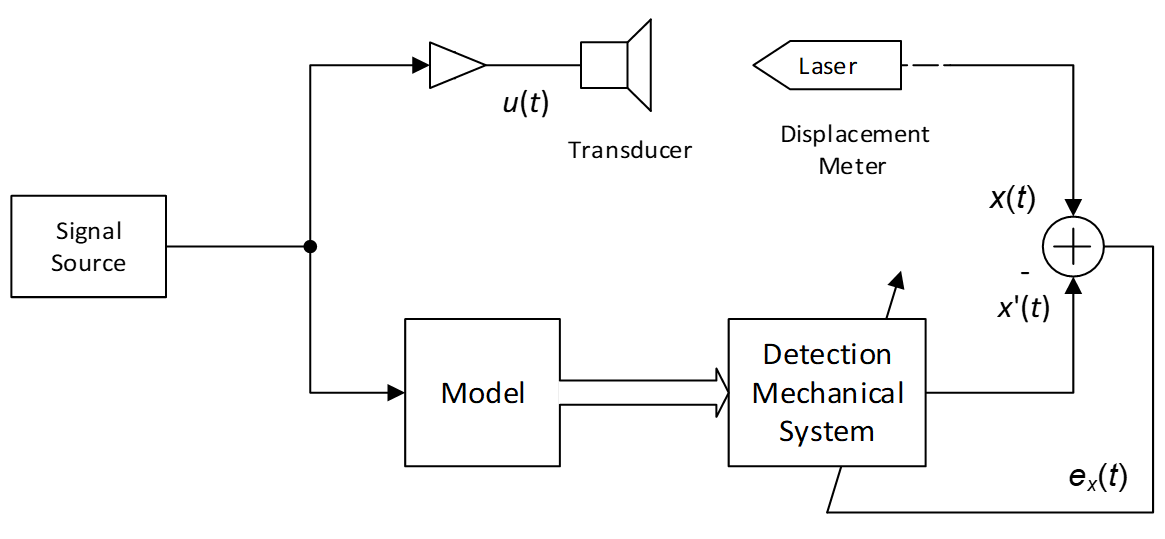
The difference between measured displacement x(t) and estimated displacement x’(t) is used as error signal \(e_{\mathrm{x}}(t) = x(t) - x'(t)\) for the adjustment of the laser. If the error is low and the measured displacement input correlates with the internally modeled state significantly, the relative parameters are automatically transferred into absolute values.
The fitting of the laser model is described by a laser error
which is the ratio between the peak value of the ex(t) and the displacement x(t) measured in the last update interval.
The error Ex(t) decreases if a laser sensor is connected to the Klippel Analyzer and adjusted to the transducer’s membrane. The residual error is mainly caused by the imperfections of the laser system (linear response, resolution, linearity) and an optimal adjustment. Please read the instructions for using the laser sensor carefully.
If the error Ex is below a threshold of 30 %, the measured displacement signal is assumed to be reliable and is used for the identification of the mechanical parameters and states in absolute values.
Variation#
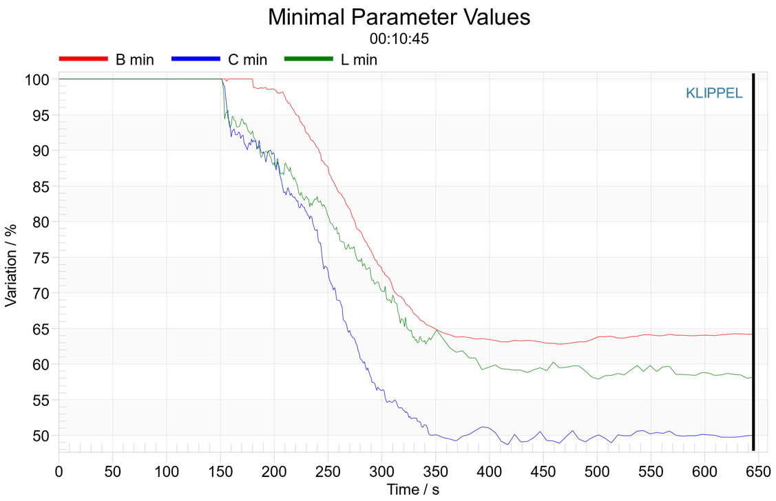
This window shows the maximum variation of the nonlinear parameters. The complicated characteristic of the nonlinear parameters is summarized to a simple single value representation by calculating the ratio of the parameter value at the minimum and at the rest position in percent, displayed versus measurement time.
These criteria are required for detecting the working range of the transducer automatically. If the allowed working range is found, the variation curves converge to specific values. These final values can also be helpful to find the dominant nonlinearity.
The time cursor can be dragged with the mouse or moved to go back in measurement history.
Minimal Compliance Ratio Cmin#
The minimal compliance ratio
is a single value representation of the nonlinear compliance neglecting the complicated shape of the curve. This value plays an important role in the determination of xmax and for the mechanical protection of the driver during the measurement.
Minimal Force Factor Ratio Blmin#
The minimal force factor ratio
is a single value representation of the nonlinear Bl-product neglecting the complicated shape of the curve. This value plays an important role in the determination of xmax and for the mechanical protection of the driver during measurement.
Minimal Inductance Ratio Lmin#
The inductance ratio
is the ratio of the minimal parameter value in the allowed working range to the value at the rest position in percent.
fs(t), Kms(t), Rms(t)#
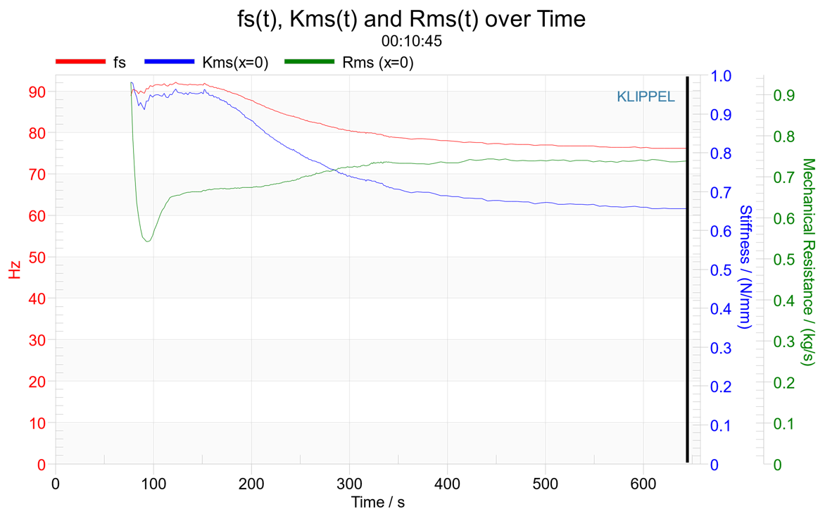
This result window shows the resonance frequency of the mechanical system fs(t,x=0), the stiffness of the mechanical suspension Kms(t,x=0) at the rest position x = 0 as well as the resistance of the mechanical suspension Rms versus measurement time t. The parameters are closely related since the moving mass Mms is assumed as constant.
Some of the parameter variations related to the mechanical suspension are reversible processes. Exposing the suspension to high excursions, the stiffness at the rest position usually decreases. Though the parameter returns to the initial value after reducing the amplitude of the excitation signal. This effect can be measured on most woofers that use conventional spider materials. The stiffness Kms(x,t) should be understood as a nonlinear system having some memory in which the stiffness depends not only on the instantaneous displacement, but also on the history of the displacement.
The time cursor can be dragged with the mouse or moved to go back in measurement history.
- LSI with Enclosure
If the enclosure setting is set to sealed or vented, both Sd and the box volume Vb at category Driver need to be set correctly.
Note that you can change Sd and Vb after the measurement is complete. However, the enclosure type must be set before the measurement.
Re(t) and Q-Factors#
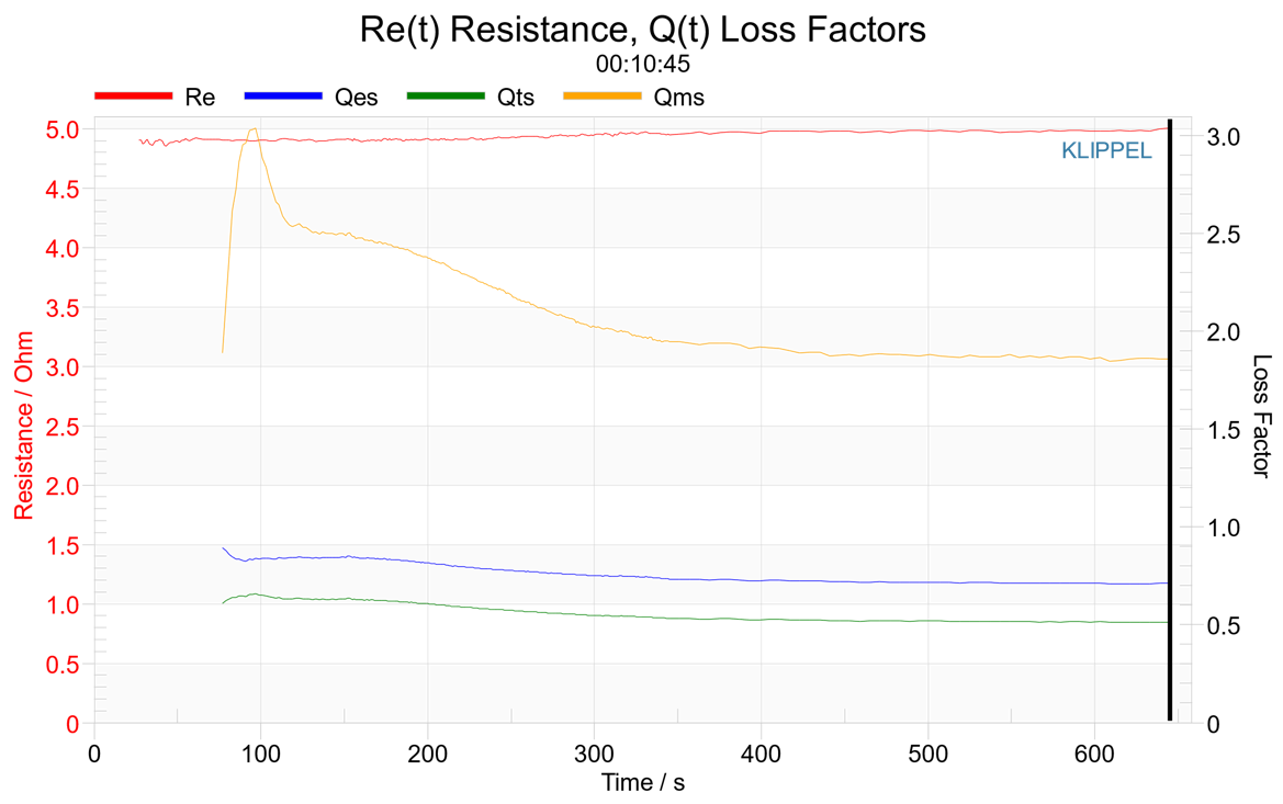
This result window shows the voice coil resistance Re(t) and the related loss factor Qes(t,x=0) at the rest position x = 0 versus the measurement time. First estimates on both parameters are available at the end of the Linear Mode. In the Enlargement Mode, the amplitude of the excitation signal is increased and both parameters rise together with the temperature of the voice coil.
The time cursor can be dragged with the mouse or moved to go back in measurement history.
Efficiency#
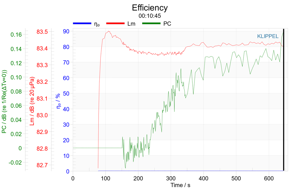
This result window shows the reference efficiency \(\eta_{0}(t)\), reference sound pressure level \(L_m(t)\) and thermal power compression factor \(PC(t)\) versus measurement time. The parameter variations are mainly caused by heating, ageing and other reversible or non-reversible changes.
The time marker can be dragged with the mouse or moved with ctrl-cursor to go back in measurement history.
Efficiency#
The reference efficiency \(\eta_{0}\) of a driver mounted in an infinite baffle and radiating into a half space free field can be calculated from the parameters at the rest position \(x = 0\)
using density \(\rho_{0}\) of air , velocity \(c\) of sound.
Considering heating of voice coil temperature versus time \(t\):
Sensitivity#
The driver mounted in an infinite baffle will produce a sound pressure level \(L_m\) for an electrical input power of 1 W at 1 m distance of
Thermal power compression#
Thermal power compression PC is calculated by considering the variation of the voice coil resistance \(R_{\text{e}}\)
Remedies for Transducer Nonlinearities#
The identified large signal parameters show the physical causes of nonlinear distortion. The characteristic of each nonlinearity can be divided into asymmetrical and symmetrical parameter variations.
The asymmetrical parameter variations produce not only second-, third- and higher-order distortion in the acoustic output signal, but also generate a DC part in the voice coil displacement that moves the voice coil dynamically out of the gap and can cause unstable behavior. If these asymmetries are either caused by an offset of the voice coil position or of the operating point in the suspension, the transducer can be easily improved at low cost.
Bl Symmetry Range#
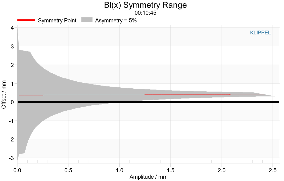
The asymmetry of the Bl curve can be evaluated by
depending on the deviation xoff from the coil’s rest position and the amplitude xac describing the positive and negative limits of the working range. A asymmetry is negligible if |ABl| < 5 %. A so called Bl symmetry region is plotted as a gray area versus xoff and xac in window Bl symmetry.
The peak displacement xBl,asym describes the amplitude xac where the ABl = 5 % for xoff = 0. If the voice coil displacement exceeds this value in the target application |x| > xBlasym, the physical cause of the Bl asymmetry should be investigated (check symmetry of the B field or the rest position of the coil).
In the example above, the voice coil offset has only a small effect as long as the peak displacement \(x < x_\mathrm{Bl,asym} =\) 1 mm.
Kms Symmetry Range#
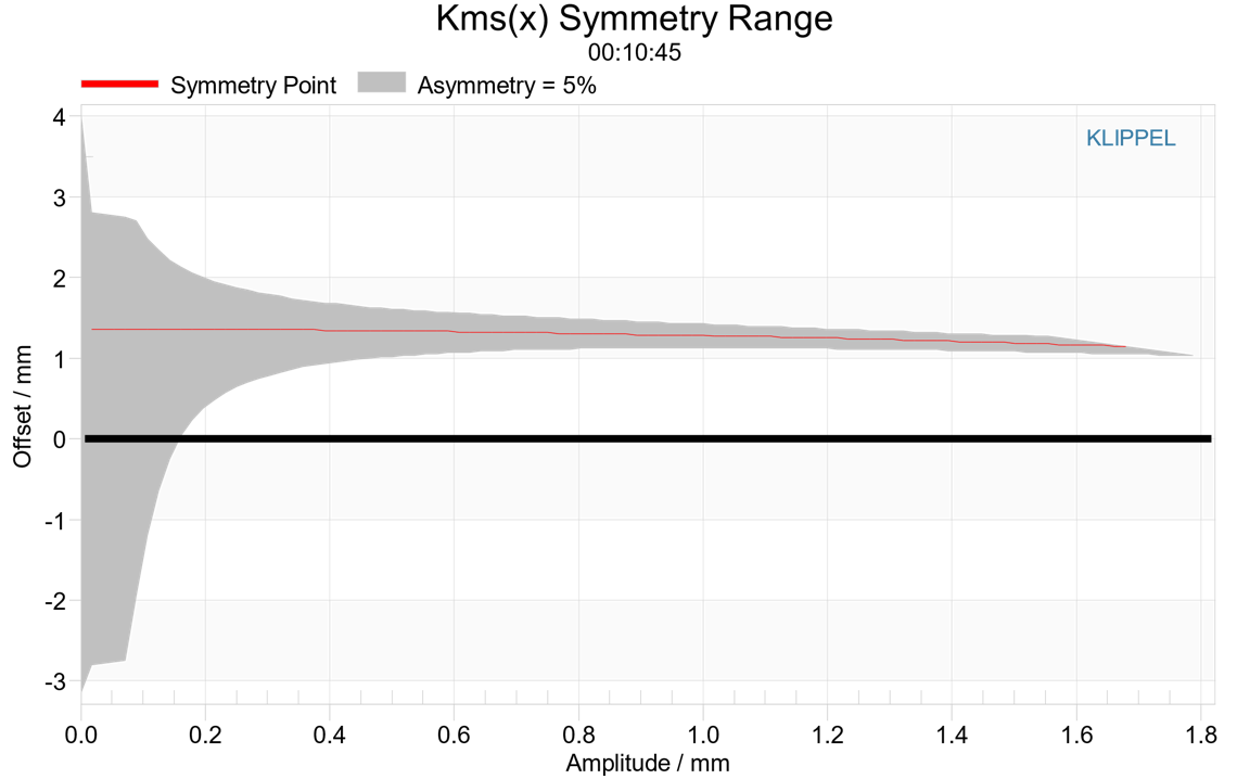
The Kms symmetry range displays the area where Kms the variation is below 5%, as function of displacement amplitude (x Axis) and voice coil offset (y axis).
In the desired working range, the x axis (y=0) should completely lie within the symmetry range (gray area). In this case, Kms asymmetries can be neglected.
The Kms asymmetry can be assessed by a single value
using the stiffness at the negative and positive peak displacement ± xpeak of the measured Kms-curve. The sign of AK corresponds with the sign of the DC displacement generated dynamically by the nonlinear rectification process.
It is a typical sign for a geometrical asymmetry of the spider (cup form) or surround (half wave profile) if the symmetry region is parallel to the x axis, but does never overlap it. A better adjustment of the suspension parts helps in some cases. Usually, the causes of the asymmetry have to be identified by separating spider and surround and using FEA.
Please find more information in the following Application Notes:
Separating Spider and Surround, AN 2
Adjusting the Mechanical Suspension, AN 3
Suspension part measurement, AN 26
Symmetry Point#
The red lines in the Bl(x) and Kms(x) symmetry range charts show their symmetry points. Ideally, the symmetry points coincide with the x axis.
The symmetry point in the nonlinear Bl(x) curve is where a negative and positive displacement x will produce the same force factor
\(Bl(x + x_\mathrm{B}(x)) = Bl(-x + x_\mathrm{B}(x))\),
with xB being the voice coil shift that symmetrizes Bl(x) for the amplitude x. The same rule applies to the Kms(x) symmetry point.
Note
The symmetry points will not be displayed in regions where it is not unique. This may occur when the nonlinear curves have multiple maxima, an unusual shape, or needs better identification.
Please find more information in the Application Notes Optimal Voice Coil Rest Position, Application Note 1 (10/2001).
Setup Parameters#

This window shows some information about the configuration.
Controlling the Time Cursor#
All time-dependent charts contain a time cursor (vertical black bar) which is typically positioned at the end of the time scale.
The cursor can be dragged with the mouse, or moved with the following keys:
- Ctrl + Cursor Left / Right
Move to previous / next sample point
- Ctrl + Home / End or Ctrl + Alt + Cursor Left / Right
Move to first / last sample
- Ctrl + Click into the diagram
Move the cursor to the nearest sample located at the mouse pointer
All other windows will follow the time cursor show the state of the measurement at the selected time. So you can inspect changes over time, and the adaption process. E.g. you can monitor the current working range (black curve in the Bl(x), Cms(x), Kms(x), Le(x) windows) changing with different amplitudes.
Tip: To visualize mechanical stiffness changes, you can set the cursor to approx. 1/3rd of the Enlargement Mode, copy the Kms(x) curve, to the clipboard, paste it back into the Kms(x) graph as passive curve, then set the time cursor back to the end of the measurement. You will see both Kms(x) curves (from early Enlargement Mode, and final) side by side.
Supported Modules for Im/Export#
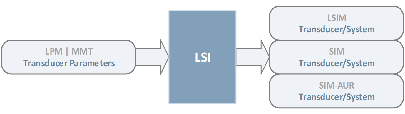
Malfunction and Troubleshooting#
Overview#
This chapter will provide information that can help you solve common problems that occur with LSI3 measurements.
If you cannot find a description here that matches your problem, try these options:
Check the Malfunction and Troubleshooting section of the dB-Lab documentation.
Check the file readme.txt that you received with your Klippel products. This document contains the most up-to-date information about products and installation procedures.
Contact Klippel support via KLIPPEL support.
Hardware Messages#
Warning and exception messages generated by the hardware unit are displayed in the State result window. Important messages are additionally displayed in a pop-up box while the measurement is running.
Low Amplifier Output#
- Cause:
The voltage measured at the output of the power amplifier is too low. Usually, the power amplifier is switched off (e.g. power saving mode) or the manual gain control is attenuated. If displayed in the Amplifier Mode (1), also a signal processing latency larger than the allowed specified maximum could cause the message.
- Remedy:
Check the power amplifier and restart the measurement.
f HP Amplifier Too High#
- Cause:
Power amplifiers usually use a high-pass filter at their input to suppress any DC voltage. Though the LSI3 Woofer uses a pilot tone at 2…4 Hz to measure the voice coil’s DC resistance. Hence it is required to amplify the pilot tone so that a sufficient level of voltage and current is reached at the transducer’s terminals. The measurement fails if the required gain is more than 20 dB to reach a sufficient level.
- Remedy:
Replace the power amplifier or disable the high-pass filter in the power amplifier. If a suitable amplifier is used, the LSI3 Woofer uses a pilot tone at 2 Hz. An acceptable amplifier will cause the LSI3 Woofer to increase the pilot tone to 4 Hz. The pilot tone frequency is listed at the State window.
No Driver Connected#
- Cause:
No valid current signal is measured or the electrical resistance of the voice coil is above the maximum limit.
- Remedy:
Check if the transducer is properly connected to the Klippel Analyzer. After starting the operation, the test signal should be audible. The voltage should be above noise level (see voltage chart).
High Fitting Error#
- Cause:
The difference (error Ei) between measured and estimated current is a measure for the fitting of model (see fitting error). A driver with regular properties which corresponds with the model produces an error of 5 … 20 %. A higher value of Ei as shown in the State window indicates a poor fitting. In most cases this is caused by a high value of the voice coil inductance or an irregular impedance response due to the para-inductance or additional modes which appear in the impdance (e.g. caused by a high acoustic impedance due to horns or panels). Additional elements such as crossover or a second transducer (tweeter) in parallel connection is not suported by the LSI3 as this is not considered in the transucer model and will increase the residual error.
- Remedy:
Make sure you have selected the correct enclosure (free air, vented) in the LSI3’s property page. Enable the automatic noise adjustment or adjust the noise manually in the Stimulus section on the SETUP property page. Remove additional electrical or acoustical elements connected to the transducer. Repeat the measurement.
High Amplifier Error#
- Cause:
The difference (error Eu) between output signal and measured voltage characterizes the performance of the amplifier (see voltage error. An amplifier with good applicability for large signal measurements produces an error of 5 … 20 %. A higher value of Eu as shown in the State window indicates a problem with the amplifier (e.g. clipping or protection modes). Additional elements such as a crossover are also not considered and will increase the residual error.
- Remedy:
Check the power amplifier and restart the measurement. Remove additional electrical elements connected to the transducer.
Wrong Amplifier#
- Cause:
A DC-coupled measurement has been started, but the DC-coupling of the amplifier could not be verified.
- Remedy:
Check the power amplifier and the setup and restart the measurement.
Maximum Output Gain#
- Cause:
The gain increase in the large signal domain by the automatic gain adjustment has reached the allowed maximum value. The protection variables have not yet exceeded the allowed protection limits.
- Remedy:
The measurement will finish using the maximum output gain that could be reached. To measure the speaker at a larger level, the measurement has to be stopped. Increase the gain of the amplifier. If that is not possible, use a power amplifier with higher gain. Then start the measurement again.
Minimal Output Gain#
- Cause:
The protection variables exceed the allowed protection limits in the small signal domain. Thus, the amplitude of the excitation signal is too high in the small signal domain.
- Remedy:
Stop the measurement. Decrease the amplitude of the excitation signal in the small signal domain by attenuating Usmall in the Stimulus section of the property page. Then restart the measurement.
Driver fs Too High#
- Cause:
The instantaneous resonance frequency of the driver is above the maximum supported value. This problem may occur if a midrange or tweeter driver is measured by using LSI3 Woofer.
- Remedy:
If you are using the LSI3 Woofer, switch to the LSI3 Micro‑speaker which is capable of measuring drivers with higher resonance frequencies, such as tweeters and micro-speakers. In some cases, it is possible to reduce the resonance frequency of the transducer by adding an additional mass to the diaphragm and to accomplish a successful measurement.
Driver fs Too Low#
- Cause:
The instantaneous resonance frequency of the driver is below the allowed minimal value. This problem may occur if a woofer is measured using the LSI3 Micro‑speaker version.
- Remedy:
If you are using LSI3 Micro‑speaker, switch to LSI3 Woofer which is capable of measuring drivers with lower resonance frequencies, such as subwoofers and woofers. In some cases, it is possible to increase the resonance frequency by placing the driver in a sealed enclosure to accomplish a successful measurement.
Temperature Too High#
- Cause:
The increase of the voice coil temperature exceeds the defined limit defined in the Protection section of the property page. That can happen if the time constant of the voice coil heating is very short and the heating is faster than the measurement.
- Remedy:
Increase the temperature limit in the protection settings if that is safe. Make sure that the stimulus settings are set to Automatic. If it is set to Manual, make sure that the Boost Resonance option is active.
Warning
If the automatic gain control is not able to keep the voice coil temperature below the defined limit, stop the measurement and restart with an adjusted electrical input power limit to prevent a thermal damage of the speaker.
Output DAC Limits#
- Cause:
The output signal of the Klippel Analyzer exceeds the allowed limit. The output signal cannot be increased further.
- Remedy:
The measurement will finish using the maximum output level reached. If you want to measure the speaker at higher excursion, stop the measurement. Increase the gain of the amplifier to provide sufficient amplitude at the speaker’s terminals in the large signal domain. Then start the measurement again.
ADC Limiting (Sensor)#
- Cause:
The peak value of the measured current or voltage signal is too high and the analog-to-digital converter is limiting.
- Remedy:
For low resistance drivers, use the low sensitivity sensors (KA3 Signal Configuration
).
Any Other Error Not Listed Above#
- Cause:
A problem in the digital signal processing has been detected.
- Remedy:
Generate a new object and repeat the measurement. Save this measurement and its settings by pressing the yellow envelope button
 in dB-Lab’s tool bar
and send the data to KLIPPEL support.
in dB-Lab’s tool bar
and send the data to KLIPPEL support.
Literature#
[1] R. H. Small, „Direct-Radiator Loudspeaker System Analysis,“ J. Audio Eng. Soc., vol. 20, pp. 383 – 395 (1972 June).
[2] R.H. Small, „Closed-Box Loudspeaker Systems, Part I: Analysis,“ J. Audio Eng. Soc., vol. 20, pp. 798 – 808 (1972 Dec.).
[3] A. N. Thiele, „Loudspeakers in Vented Boxes: Part I and II,“ in Loudspeakers, vol. 1 (Audio Eng. Society, New York, 1978).
[4] J. R. Ashley and M. D. Swan, „Experimental Determination of Low-Frequency Loudspeaker Parameters“ in Loudspeakers, vol.1 (Audio Eng. Society, New York, 1978).
[5] R. H. Small, “Assessment of Nonlinearity in Loudspeakers Motors,” in IREECON Int. Convention Digest (1979 Aug.), pp. 78-80.
[6] M.R. Gander, “Moving-Coil Loudspeaker Topology as an Indicator of Linear Excursion Capability,” in Loudspeakers, vol.2 (Audio Engineering Society, New York, 1984).
[7] A. Dobrucki, C. Szmal, “Nonlinear Distortions of Woofers in Fundamental Resonance Region,” presented at the 80th convention Audio Eng. Soc., Montreux, March 4-7, 1986, preprint 2344.
[8] C. Zuccatti, “Thermal Parameters and Power Ratings of Loudspeakers,” J. Audio Eng. Soc., vol. 38, pp. 34 – 39, (Jan./Feb. 1990).
[9] D. Button, “A Loudspeaker Motor Structure for Very High Power Handling and High Linear Excursion,” J. Audio Eng. Soc., vol. 36, pp. 788 – 796, (October 1988).
[10] C. A. Henricksen, “Heat-Transfer Mechanisms in Loudspeakers: Analysis, Measurement, and Design,” J. Audio Eng. Soc., vol. 35, pp. 778 – 791, (October 1987).
[11] W. Klippel, “Dynamic Measurement and Interpretation of the Nonlinear Parameters of Electrodynamic Loudspeakers,” J. Audio Eng. Soc., vol. 38, pp. 944 - 955 (1990).
[12] E. R. Olsen and K.B. Christensen, “Nonlinear Modeling of Low Frequency Loudspeakers - a more complete model,” presented at the 100th convention Audio Eng. Soc., Copenhagen, May 11-14, 1996, preprint 4205.
[13] M.H. Knudsen and J.G. Jensen, “Low-Frequency Loudspeaker Models that Include Suspension Creep,” J. Audio Eng. Soc., vol. 41, pp. 3 - 18, (Jan./Feb. 1993).
[14] A. Dobrucki, “Nontypical Effects in an Electrodynamic Loudspeaker with a Nonhomogeneous Magnetic Field in the Air Gap and Nonlinear Suspension,” J. Audio Eng. Soc., vol. 42, pp. 565 - 576, (July./Aug. 1994).
[15] A. J. M. Kaizer, “Modeling of the Nonlinear Response of an Electrodynamic Loudspeaker by a Volterra Series Expansion,” J. Audio Eng. Soc., vol. 35, pp. 421-433 (1987 June).
[16] W. Klippel, “Nonlinear Large-Signal Behavior of Electrodynamic Loudspeakers at Low Frequencies,” J. Audio Eng. Soc., vol. 40, pp. 483-496 (1992).
[17] J.W. Noris, “Nonlinear Dynamical Behavior of a Moving Voice Coil,” presented at the 105th Convention of the Audio Engineering Society, San Francisco, September 26-29, 1998, preprint 4785.
[18] W. Klippel, “The Mirror Filter - A New Basis for Reducing Nonlinear Distortion and Equalizing Response in Woofer Systems,” J. Audio Eng. Soc., vol. 40, pp. 675 - 691 (1992).
[19] J. Suykens, J. Vandewalle and J. van Gindeuren, “Feedback Linearization of Nonlinear Distortion in Electrodynamic Loudspeakers,” J. Audio Eng. Soc., Vol. 43, No. 9, pp. 690-694 (1995).
[20] W. Klippel, “Direct Feedback Linearization of Nonlinear Loudspeaker Systems,” J. Audio Eng. Soc., Vol. 46, pp. 499-507 (1995 June).
[21] H. Schurer, C. H. Slump, O.E. Herrmann, “Theoretical and Experimental Comparison of Three Methods for Compensation of Electrodynamic Transducer Nonlinearity,” Audio Eng. Soc., Vol. 46, pp. 723-739 (1998 September).
[22] W. Klippel, “Adaptive Nonlinear Control of Loudspeaker Systems,” J. Audio Eng. Soc. vol. 46, pp. 939 - 954 (1998).
[23] F.Y. Gao, “Adaptive Linearization of a Loudspeaker,” presented at 93rd Convention of the Audio Eng. Soc., October 1 -4, 1992, San Francisco, preprint 3377.
[24] W. Klippel, “Nonlinear Adaptive Controller for Loudspeakers with Current Sensor,” presented at the 106th Convention of the Audio Engineering Society, Munich, May 8-11, 1999, preprint 4864.
[25] W. A. Frank, “An Efficient Approximation to the Quadratic Volterra Filter and its Application in Real-Time Loudspeaker Linearization,” Signal Processing, vol. 45, pp. 97-113, (1995).
[26] D. Clark, „Precision Measurement of Loudspeaker Parameters,“ J. Audio Eng. Soc. vol. 45, pp. 129 - 140 (1997 March).
[27] E. Geddes and A. Philips, “Efficient Loudspeaker Linear and Nonlinear Parameter Estimation,” presented at the 91st Convention of the Audio Engineering Society, J. Audio Eng. Soc. (Abstracts), vol. 39, p. 1003 (1991 Dec.), preprint 3164.
[28] D. Clark and R. Mihelich, “Modeling and Controlling Excursion-Related Distortion in Loudspeakers,” presented at the 106th Convention of the Audio Engineering Society, Munich, May 8-11, 1999, preprint 4862.
[29] D. Clark, “Amplitude Modulation Method for Measuring Linear Excursion of Loudspeakers,” presented at the 89th Convention of the Audio Engineering Society, J. Audio Eng. Soc. (Abstracts), vol. 38, p. 874 (1990 Nov.), preprint 2986.
[30] G. Cibelli, A. Bellini, E. Ugolotti, “Dynamic measurements of low-frequency loudspeakers modeled by Volterra series,” in preprint 4968 presented on 106th Convention of the Audio Eng. Soc., Munich, May 8-11, 1999.
[31] M. Knudsen, “Estimation of Physical Parameters in Linear and Nonlinear Dynamic Systems, Ph. D. dissertation, Aalborg University, Department of Control Engineering, ISNN 0106-0791, AUC-CONTROL- R93 – 4010, January 1993.
[32] M. Knudsen, J.G. Jensen, V. Julskjaer and P. Rubak, “Determination of Loudspeaker Driver parameters Using a System Identification Technique,” J. Audio Eng. Soc. vol. 37, No. 9.
[33] G.L. Beers and H. Belar, “Frequency-Modulation Distortion in Loudspeakers,” J. Audio Eng. Soc. vol. 29, pp. 320 –326, (1981 May)
