At higher amplitudes, loudspeakers generate significant distortion due to nonlinearities inherent in the transducer.
The FLSI measurement module identifies these nonlinearities using a fully dynamic measurement technique and links
them to specific physical mechanisms, design choices, material properties, and assembly processes.
This allows FLSI to reveal the true physical causes of distortion, not just their symptoms.
It provides valuable insight into the loudspeaker’s physical behavior — crucial for design verification,
defect detection, and optimization in terms of sound quality, weight, size, and cost.
Engineers can instantly identify dominant nonlinearities and focus development where it matters most.
FLSI is the result of decades of research in nonlinear system identification and loudspeaker modeling and
represents the next-generation evolution of small- and large-signal identification.
It is the successor to the R&D modules LPM and LSI3.
While the traditional approach using LPM and LSI provides valuable small- and large-signal parameters,
FLSI goes significantly further by delivering a more complete and more accurate loudspeaker model in a single, fully automated measurement.
This eliminates the need for multiple tools, reduces overall test complexity, and ensures consistent small- and large-signal measurement results.
See FLSI homepage
for an overview of features and benefits of FLSI compared to LPM and LSI.
FLSI is available in two versions:
FLSI Pro: State-of-the-art measurement technology with the full feature set.
FLSI Standard: Based on the same state-of-the-art measurement technique, providing a parameter set comparable to LPM and LSI3. Not all features described in this document are included in the Standard version.
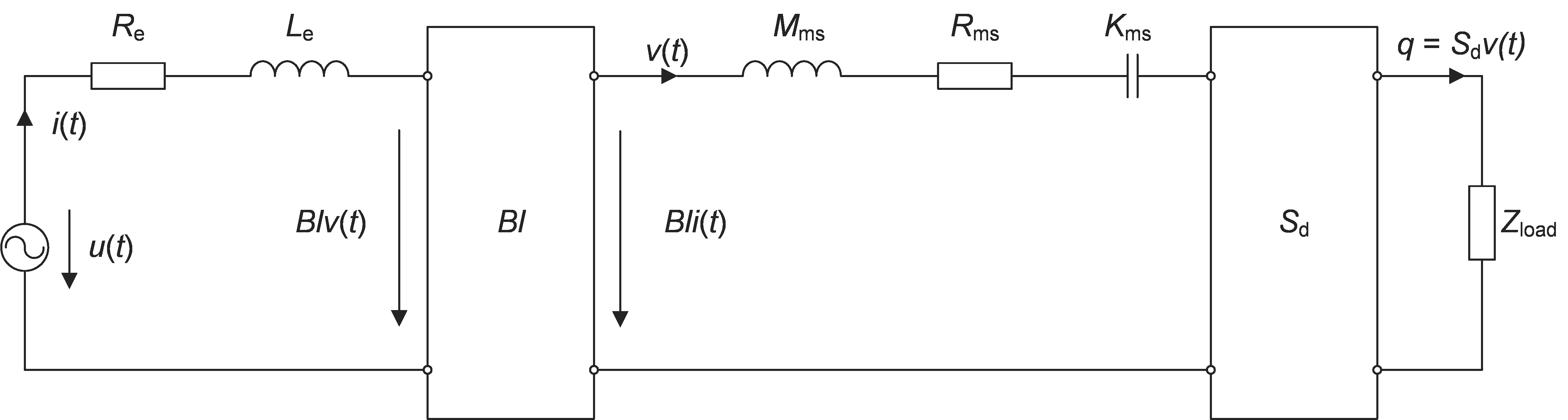
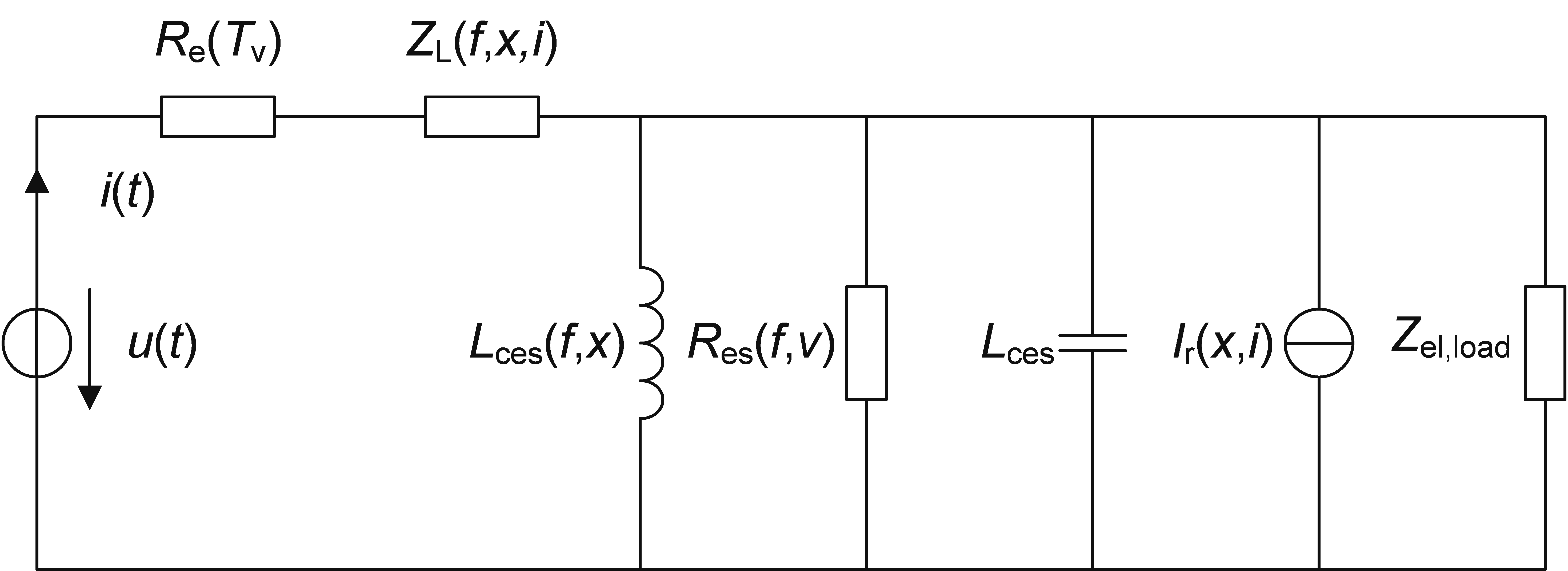
Both use a lumped parameter model similar to the one shown below to represent the loudspeaker.
This model does not only comprise linear parameters, but many nonlinear parameters
that depend on system states such as displacement and velocity.
For example, the force factor depends on voice coil position, while nonlinear air flow resistance depends on velocity.
Internet access is required for parameter identification on the FLSI Server.
See Network Configuration for information about the server communication and network configuration.
See our Privacy Policy below, explaining why a parameter identifications happens on a server and which data is exchanged.
Single electro-dynamic moving-coil or moving-magnet transducers in free air, or mounted in an enclosure that can be modeled with a 4th order filter function (i.e., closed, vented, passive radiator).
Not supported are:
Passive crossovers connected to the transducer.
Multiple transducers connected in parallel or in series.
Speakers with complex mechanical or acoustical loads (i.e., bandpass systems of order 6 and higher, or shakers mounted on free-swinging boards causing many distinct peaks in the electrical impedance magnitude)
Active speakers without access to the transducer terminals.
Transducers not operating according to the electro-dynamic moving-coil or moving-magnet principle.
FLSI can create initial data for Klippel Controlled Sound (https://www.klippel.de/go/kcs).
The according entries on FLSI’s property page are only available when a KCS-ID license is installed.
KCS data creation requires a successfully finished THERMAL MODE (available in FLSI Pro and FLSI Standard with KCS-ID license).
In addition, it is highly recommended to use a microphone to measure \(S_\mathrm{d}(x)\) (Measuring Sd(x)).
Note
In case you have an existing FLSI and have installed the KCS-ID license,
it is required to trigger FLSI module’s license check by changing a parameter on the property page.
I.e., temporarily change the entry of the Geometry drop-down list.
For more information and KCS data creation troubleshooting, also see
KCS-ID’s manual.
The hardware setups on the KLIPPEL KA3 comprising one Speaker Card, one Laser Card, one XLR
Card, and an optional AMP Card is illustrated in the figures below. For more information
about the hardware, please see the hardware manual.
Connect the DUT (device under test) to the SP 1 or SP 2Speakon connectors of the KA3’s Speaker Card.
Note
Make sure that the the DUT is fixed securely and connected tightly — it must not move around during the measurement.
Also alligator clips can corrode over time, especially in humid areas, and
their springs can wear out, which leads to loose connections.
The FLSI notices loose connections by analyzing the voltage and current signals
and will display an error message.
In this case, it might be necessary to replace them.
Laser and microphone sensors are not necessarily required for operating the FLSI.
However, these sensors are highly recommended to get a comprehensive set of diagnostics information.
The laser measures the voice coil’s peak displacement, which is then used to automatically determine the force factor Bl(x=0)
(see Mechanical and Acoustical Calibration).
The microphone measures impulsive distortion, which can be used as a protection limit,
and nonlinear distortion, which provides information about the harmonic and intermodulation distortion
created by the deformation of the surround.
The microphone should be placed in the speaker’s near-field (see Measuring Sd(x)).
Make sure that IEPE/phantom power is switched on by pressing the buttons next to the microphone connectors on the KA3’s front panel.
Hardware connection on KA3 with AMP CardHardware connection on KA3 without AMP Card
In the dB-Lab software’s tool bar, open the KA3 Signal Configuration to setup the
routing. Set the correct output channel (AMP card or XLR Card if an external
amplifier is used) and input channels for the optional external sensors.
Open a database by pressing Select Database in the dB-Lab software. Create a new
FLSI Fast Large Signal Identification operation, open its Properties by right-clicking on the operation and set up the
measurement as follows. It is assumed that the hardware is set up as described in Hardware Configuration
and the laser and the microphone are connected to the KA3.
Select which sensors are connected in the Peripherals category. This is required for the measurement module
to decide which protection parameters are available.
In the KA3 Routing category, select which in- and output channels of the hardware device shall be used.
Incorrect settings may damage the driver.
Be especially careful with tweeters, micro-speakers, and telecommunications drivers.
For these devices, consider reducing the Start Voltage on the property page if the default value may already drive the device close to its limits.
For fragile or expensive prototypes with unknown peak displacement capability, it is recommended to set the NONLINEAR MODE level manually (e.g., starting at 1 V)
and increase it gradually in small steps, since fragile transducers may already be damaged when impulsive distortion protection limit is triggered.
Impulsive Distortion
A microphone is required to use this part of the protection system.
The impulsive distortion is identified by exploiting out-of-band distortion in the sound pressure signal.
The crest factor \(CID_\mathrm{MT}\) of the out-of-band distortion is calculated.
High \(CID_\mathrm{MT}\) values indicate that the speaker is working above its safe working range.
Note that the impulsive distortion metric \(CID_\mathrm{MT}\) is calculated similarly
to the \(CID\) for sinusoidal excitation (see the TRF Transfer Function module).
However, the crest factor of the multi-tone is higher than that of the sinusoidal tone.
Therefore, multi-tone’s impulsive distortion limit is higher than the sinusoidal excitation’s one.
Note
The Impulsive Distortion limit is very valuable in many cases to determine a safe maximum
voice coil displacement. However, if there is background noise, parasitic vibrations e.g. originating from the speaker
stand or rattling objects in the room, this protection system will trigger already at low displacements
where the speaker might still behave linearly and the nonlinear parameter variations are low.
In this case, use other protection parameters such as \(X_\mathrm{target}\) and deactivate the Impulsive Distortion protection.
X target
This parameter specifies the maximum absolute peak voice coil displacement
that shall be used in the measurement.
The peak displacement value is measured by a laser sensor.
Note
The voice coil’s rest position is measured at the very beginning of the LINEAR MODE.
Ensure that the positions of the DUT and the laser remain unchanged throughout the entire measurement.
Relative Bl(x) min
The minimal force factor ratio \(Bl_\mathrm{min}(x)\) is a useful criterion to detect the
maximum displacement \(x_\mathrm{max}\) of the voice coil.
This parameter reflects the ratio of the
voice coil height to the thickness of the pole plates in the motor structure. A low minimal force factor
ratio, e.g. \(Bl_\mathrm{min}(x) < 50%\) produces substantial distortion components in the output signal
spreading over the whole excited frequency band and indicates the end of the useable working
range.
The default value might be decreased if the driver is capable and intended to be used in a more nonlinear region.
Increase this value if the DUT is fragile or it has a very high voice coil overhung.
Relative C(x) min
The minimal compliance ratio \(C_\mathrm{min}(x)\) describes the geometrical changes of the suspension.
A high decrease of the compliance, e.g. to \(C_\mathrm{min}(x)\) < 50%, produces
substantial harmonic distortion components in the output signal and
indicates the end of the useable working range.
The default value might be decreased, if the driver is capable and intended to be used in a more nonlinear region.
Note
The working range of tweeters, headphones, micro-speakers and other transducers without
spider is usually not limited by a progressive mechanical stiffness.
For these speaker types, it is recommended to activate the impulsive distortion limit.
In addition, the maximum displacement \(X_\mathrm{target}\) limit or a conservative manually entered excitation voltage might be used.
This ensures that the transducer operates in its permissible working range and avoids
damage due to hard limiting.
Coil Temperature
This protection limit defines the maximum allowed relative voice coil temperature increase. If this limit is
exceeded, the measurement is immediately stopped to avoid permanent voice coil damage.
The measurement of the coil temperature is done by
measuring its DC resistance using a low frequency tone \(f_\mathrm{Re}\).
The reference temperature is measured at the beginning of the LINEAR MODE.
Make sure that the voice coil temperature is at approx. room temperature at the beginning of the measurement.
Note
Voice coils do not heat up homogeneously. Usually, the hottest place is at the rims, while
it is cooler in the gap. The FLSI measures the average temperature. Hence, allow some margin to the
maximum absolute maximum temperature rating of the voice coil.
Make sure that the environment is quiet during the measurement to avoid the transducer acting as a microphone, creating undesired distortion in the back-EMF.
When performing the first measurement of a speaker model, it is recommended to firstly determine the peak displacement and
optimal measurement settings (e.g., excitation voltages) automatically,
following the procedure outlined in FLSI Software Configuration.
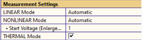
If the speaker is large and can cope with higher powers, the setting Start Voltage (Enlargement Mode)
can be increased on the operation’s property page.
This will accelerate the ENLARGEMENT MODE, allowing it to start at a higher voltage.
If the thermal parameters of the DUT are known or not relevant,
the THERMAL MODE can be deactivated to further reduce measurement time
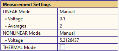
If the DUT or a device with the same design has been characterized previously,
you can switch the LINEAR and NONLINEAR MODE settings from Automatic to Manual.
In this case, the automatic level determination in the LINEAR MODE and ENLARGEMENT MODE will be skipped.
This is particularly useful when measuring multiple samples of the same speaker model.
The protection system, except the thermal protection, is inactive in manual mode.
Ensure that the transducer can handle the given voltage.
Note
Tip: If you set the settings to Manual on an already existing operation that holds result data,
the property page displays the settings (i.e., excitation level and number of averages) of the previous measurement.
Automatic Measurement SettingsManual Measurement Settings skipping ENLARGEMENT and THERMAL MODE
FLSI identifies both linear and nonlinear parameters, as well as state information of the transducer.
In addition to the Thiele-Small parameters that are valid only at small amplitudes,
it identifies parameters that describe the nonlinear behavior over the
entire transducer’s working range.
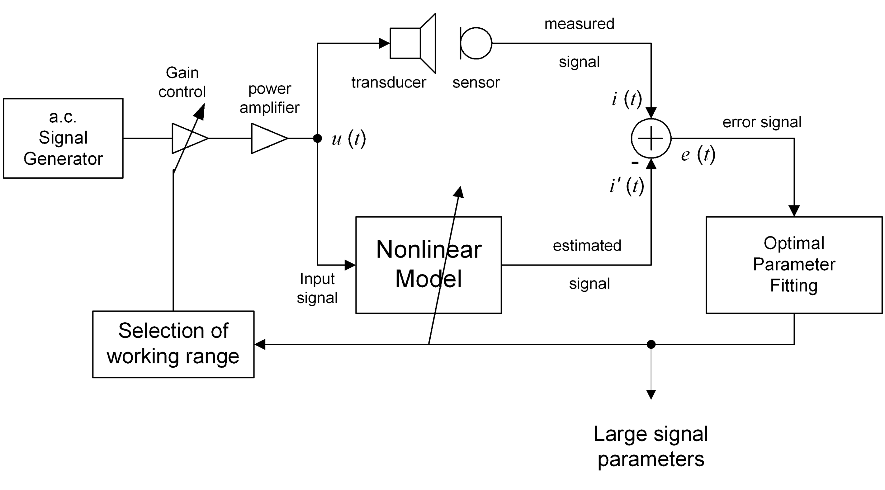
FLSI measures the free parameters of an extended loudspeaker model
using a full dynamic measurement. The loudspeaker is excited with a frequency-shaped multi-tone stimulus.
The stimulus bandwidth is determined automatically by measuring the DUT’s resonance frequency,
approximately covering the bandwidth relevant to the target application.
Additionally, a low-frequency tone is applied to measure the DC resistance, which is necessary for tracking the
voice coil temperature required for thermal protection and the identification of the
thermal model.
Optimal parameters are estimated by a nonlinear system identification algorithm,
primarily based on the voltage and current signals available at the loudspeaker terminals.
Full dynamic measurement (IEC 62458)
In addition to measuring the electrical signals, an optional laser sensor should be used to measure displacement
and identify the force factor \(Bl(x=0)\) (see Mechanical and Acoustical Calibration).
A microphone can be used to approximate the nonlinear distortion contribution due to the modulation of
the transducer’s effective surface area \(S_\mathrm{d}(x)\) (see Distortion Components).
The total harmonic and intermodulation distortion of each modeled nonlinear mechanism in the loudspeaker
is calculated for the used multi-tone excitation signal.
This enables the detection of the physical cause of the
dominant distortion.
This information is crucial for identifying the weakest points in the loudspeaker design and providing insights for potential improvements.
Some nonlinear distortion can be reduced without increasing the speaker’s cost.
For example, distortion caused by asymmetries in the parameter characteristics can be minimized by
optimally centering the voice coil and mechanical suspension.
The full nonlinear transducer model serves as the basis for numerical simulations to predict
the transducer’s nonlinear behavior in various applications
(SIM, SIM‑AUR modules).
To measure the linear and nonlinear parameters of a loudspeaker driver,
it is recommended to first measure it in free air with the loudspeaker axis pointing horizontally
to prevent gravity from shifting the voice coil’s rest position.
A loudspeaker stand, such as the Klippel Pro Driver Stand or Klippel Micro-Speaker Clamping,
simplifies mounting and provides easy access for the triangulation laser.
If a large driver mounted in an enclosure needs to be measured,
a stand may be impractical due to its limited size and the potential for rattling, as significant forces are involved.
In this case, the loudspeaker can be fixed to the floor and decoupled from the laser sensor.
Ensure that the speaker remains stationary during the measurement.
Transducers must be measured under conditions that ensure the mechanical system,
including any acoustical load, can be represented as a second- or fourth-order system (see Speaker System Modeling).
Higher order systems are currently not supported.
It is recommended to measure the DUT in free air, as this requires less electrical input power and produces a
lower sound pressure level compared to measuring the same driver in a closed system.
However, the FLSI allows for the measurement of parameters in closed and fourth-order speaker systems,
such as vented, bandpass, or passive radiator systems.
This is especially useful for determining the dominant nonlinear distortion components in a loudspeaker
system with an enclosure similar to that used in the final product.
Additionally, the FLSI can identify enclosure parameters, such as the linear parameters
of the full fourth-order system (e.g., port resonance frequency and Q-factor), or the nonlinear distortion caused by the port.
The effective radiation area \(S_\mathrm{d}(x=0)\) can vary over the voice coil displacement \(x\)
due to the deformation of the surround (see Mechano-acoustical transduction).
The nonlinear distortion caused by the variation in \(S_\mathrm{d}(x)\) is approximated by exploiting information found in
the sound pressure signal, which is measured by a microphone.
For the highest precision, the distance from the microphone to the transducer’s cone should be approximately
1 to 2 times the transducer cone’s diameter.
It is possible to calculate the \(S_\mathrm{d}(x)\) distortion in a free-air measurement.
However, the sound pressure signal is linearly
distorted by the acoustical shortcut between the front and the rear of the transducer’s cone and surround.
To obtain the \(S_\mathrm{d}(x)\) distortion spectrum that corresponds as closely as possible to the final application,
we recommend performing the measurement with the transducer mounted in an enclosure.
Measurement of the linear parameters in the small signal domain
2
ENLARGEMENT MODE
Identification of the allowed working range
3
NONLINEAR MODE
Identification of the nonlinear parameters
4
THERMAL MODE
Identification of thermal parameters
LINEAR MODE:
Before driving the loudspeaker with an excitation signal, all equipment is checked for potential issues, such as
correctly connected device under test
amplifier gain
inner amplifier resistance
If any issues are detected, an error message is displayed, and the measurement is canceled.
Next, multiple measurements are performed to determine the optimal small-signal stimulus settings
(excitation voltage, number of averages, signal bandwidth).
The small-signal parameters are identified based on the measured voltage, current, and displacement (optional) signals.
ENLARGEMENT MODE (optional):
After a successful linear parameter estimation, the nonlinear parameters are estimated in the large signal domain by
gradually increasing the amplitude of the excitation signal until one of the protection criteria reaches its predefined limit.
The ENLARGEMENT MODE is divided into two parts:
The first part uses very short stimuli to roughly determine the transducer’s limit.
Once a protection limit is nearly reached or exceeded, the second part of the ENLARGEMENT MODE begins.
A longer stimulus, more similar to the NONLINEAR MODE’s stimulus, is applied to precisely
determine the transducer’s physical operating limit.
If the protection limits \(Bl_\mathrm{min}\) or \(C_\mathrm{min}\) (see 3. Select the Protection Parameters) are active,
a fast nonlinear parameter identification is performed after each measurement step.
Note that the resulting parameters may not have the highest precision, as this mode prioritizes maximum speed.
NONLINEAR MODE (optional):
After determining the optimal range of operation, the nonlinear parameters are identified using
the optimal stimulus settings (excitation voltage, bandwidth) with the highest accuracy.
THERMAL MODE (optional):
This mode identifies the short-term thermal parameters.
The voice coil is excited by a multi-tone signal with high power until its temperature is sufficiently
high to reliably determine the thermal parameters.
If the voice coil was already sufficiently heated during the NONLINEAR MODE, this heating phase might be skipped.
Afterward, the voice coil is cooled down. Based on the heating and cooling characteristics, the
thermal parameters are identified.
Linear and nonlinear loudspeaker behavior produces substantial linear and nonlinear distortion in the output signal.
These effects are closely related to the transducer’s design principles, material properties, and assembly techniques, and can be predicted using nonlinear modeling.
The FLSI R&D module combines linear and nonlinear measurement techniques with nonlinear physical simulation algorithms.
It explains the generation of distortion, identifies the underlying physical causes, and provides suggestions for constructional improvements.
This information helps to better understand the linear and nonlinear mechanisms acting in the loudspeaker,
enabling further optimization of the speaker with respect to sound quality, weight, size, and cost.
At low frequencies, an electro-mechanical equivalent circuit with lumped elements can successfully model electrodynamic transducers.
The structure of this model represents the transducer principle and the basic physical mechanisms within the transducer.
The free parameters of the model vary depending on:
The linear electrodynamic transducer model provides a simplified description of moving-coil loudspeakers
under the assumption of small-signal operation —
all parameters are considered constant and independent of displacement, velocity, current, and temperature.
The model couples an electrical subsystem to a mechanical subsystem through an ideal electromechanical transformer.
where \(u(t)\) is the applied terminal voltage, \(i(t)\) the voice-coil current, \(R_\mathrm{e}\) the DC resistance,
\(L_\mathrm{e}\) the voice-coil inductance, \(Bl\) the force factor (assumed constant in the linear model),
and \(Bl\, v(t)\) the back electromotive force (EMF).
where the parameters are the moving mass \(M_\mathrm{ms}\), the mechanical resistance (losses) \(R_\mathrm{ms}\), and the mechanical stiffness \(K_\mathrm{ms}\).
The states are the displacement \(x(t)\), the velocity \(v(t) = \dot{x}(t)\), and the acceleration \(a(t) = \ddot{x}(t)\).
In the frequency domain (\(s = j\omega\)), the mechanical impedance is
\[Z_{\mathrm{m}}(s) = R_{\mathrm{ms}} + s M_{\mathrm{ms}} + \frac{K_{\mathrm{ms}}}{s}.\]
The electrical input impedance of the transducer becomes
\[Z_{\mathrm{e}}(s) = R_\mathrm{e} + s L_\mathrm{e} + \frac{(Bl)^2}{Z_{\mathrm{m}}(s)}.\]
This expression illustrates the electromechanical coupling: mechanical resonance and losses are reflected into the electrical domain via the squared force factor.
The linear model assumes small excursions, constant force factor, linear suspension stiffness, linear damping,
and negligible magnetic saturation and thermal effects.
Despite these simplifications, it is very valuable for loudspeaker analysis and linear system design.
However, significant deviations from this model at higher signal levels motivate the introduction of nonlinear and time-varying extensions:
For an ideal coil, the inductance can be modeled using a constant inductance parameter \(L\).
The electrical impedance of the ideal inductance is
\[\underline{Z}_\mathrm{L,ideal}(f) = 2\pi f j L.\]
However, since the voice coil is surrounded by permeable and conductive materials,
its self-inductance cannot be modeled as a simple, ideal inductance.
This is due to iron losses arising from eddy currents, the skin effect, and magnetic hysteresis.
Additionally, conductive materials in the motor, such as copper caps or shorting rings, reduce the self-inductance
depending on frequency.
As a result, the linear complex impedance of the lossy inductance, valid in the small signal domain,
becomes frequency-dependent and comprises a reactive part
\(L(f)\) and a resistive part \(R_\mathrm{L}(f)\) (both are real-valued, frequency-dependent parameters).
\[\underline{Z}_\mathrm{L,linear}(f) = 2\pi f j L(f) + R_\mathrm{L}(f).\]
Section Lossy Inductance explains how the small signal lossy inductance
is displayed in FLSI.
In addition, the magnetic flux path changes depending on the voice coil’s position:
When the voice coil moves deeper into the gap toward the back plate, it becomes more surrounded by iron,
and the magnetic field lines pass predominantly through this high-permeability material.
This increases the inductance and iron losses.
Conversely, when the coil moves outward (away from the backplate) a larger portion of the magnetic field lines
passes through air, which has a relative permeability close to unity.
This reduces the inductance and iron losses.
The self-inductance also varies with the electrical current \(i(t)\) due to the nonlinear magnetization
behavior of the surrounding ferromagnetic material (iron) in response to the AC magnetic field
(see Flux Modulation).
Hence, the impedance of the inductance is frequency-dependent and nonlinear
(also see Lossy Inductance (x)):
\[\underline{Z}_\mathrm{L}(f,x,i) = 2\pi f j L(f,x,i) + R_\mathrm{L}(f,x,i).\]
In addition to the high-frequency intermodulation distortion caused by this nonlinear behavior,
the non-uniform distribution of the alternating magnetic field along the voice coil’s axis of motion generates a reluctance force \(F_\mathrm{r}\).
For an ideal, lossless inductor described by the impedance \(\underline{Z}_\mathrm{L,ideal}(x)\) which depends solely on displacement,
this force can be calculated as
The nonlinear distortion generated by this force is displayed in Distortion Components.
The reluctance force can cause a significant DC displacement, shifting the voice coil towards the highest nonlinear inductance \(L(f, x)\).
The DC forces generated by nonlinearities such as the reluctance force are displayed in the table
Nonlinear Parameters under Distortion Components.
As explained in Small-Signal Modeling, the electro-mechanical transduction parameter (force factor)
converts the current into the Laplace force.
\(Bl\) was assumed to be constant in the small-signal modeling.
However, in the large-signal domain, it can vary significantly with voice coil displacement \(x\)
(see Force Factor Bl(x)).
The shape of the nonlinearity depends on the voice coil-gap configuration (i.e., overhung, underhung, equal length).
The electromagnetic (Laplace) force acts on a spring–mass–damper system, forming the mechanical resonator of the transducer.
While the moving mass \(M_\mathrm{ms}\) is generally assumed to be constant with respect to
displacement, velocity, time, frequency, and temperature,
the suspension typically consists of highly nonlinear and lossy materials such as impregnated cloth and rubber.
As a result, the mechanical stiffness \(K_\mathrm{ms}(t, f, x)\) and mechanical resistance \(R_\mathrm{ms}(t, f, v, F)\) can vary significantly:
\(K_\mathrm{ms}\) and \(R_\mathrm{ms}\) are frequency-dependent due to mechanical creep.
\(K_\mathrm{ms}\) depends on the voice coil displacement\(x\) (see Mechanical Stiffness Km(x)) caused by deformation of the spider and surround.
\(K_\mathrm{ms}\) and \(R_\mathrm{ms}\) are time-variant reflecting suspension deformation and energy losses; their values can differ significantly between small- and large-signal conditions (see Linear Parameters at x=0).
\(R_\mathrm{ms}\) depends on the voice coil velocity\(v\) due to the air flow resistance in the motor structure (particularly relevant in smaller transducers, see Mechanical Resistance Rms(v).
\(R_\mathrm{ms}\) depends on the excitation force and time (\(F\) and \(t\)) due to internal damping mechanisms such as nonlinear creep, mechanical hysteresis, and — in moving magnet transducers — losses in the magnetic suspension.
The nonlinear distortion generated by these effects can be analyzed using the distortion components (see Distortion Components).
The transducer cone, with an effective surface area \(S_\mathrm{d}(x)\), converts velocity into volume velocity:
\[q(t) = S_\mathrm{d}(x), v(t)\]
This volume velocity generates the radiated sound pressure \(p(t)\).
The effective surface area \(S_\mathrm{d}(x)\) can vary with voice coil displacement \(x\) due to deformation of the surround.
This introduces a nonlinear radiation behavior.
The effect can become dominant when the surround area is large relative to the cone area.
This is commonly observed in small transducers (e.g., microspeakers) and in woofers designed for high excursion.
The distortion generated by this mechanism is included in the distortion components (see :ref:kl-fastlsi-distortion-components).
The nonlinearity \(S_\mathrm{d}(x)\) is identified using a microphone.
Further details on the measurement conditions can be found here.
If the transducer is mounted in an enclosure instead of being operated in free air, a load impedance
Zload must be considered, as this changes the total system response.
This load impedance can be nonlinear and generate additional nonlinear distortion.
E.g., a port in a vented box will create nonlinear distortion due to the nonlinear
air flow resistance.
In passive radiators, the nonlinear suspension stiffness will create additional nonlinear distortion at
low frequencies, comparable with the nonlinear suspension suspension of electro-dynamic transducers.
See Speaker System Modeling for acoustic load modeling.
In addition to the lumped parameters of the electrical, mechanical, and acoustical domain,
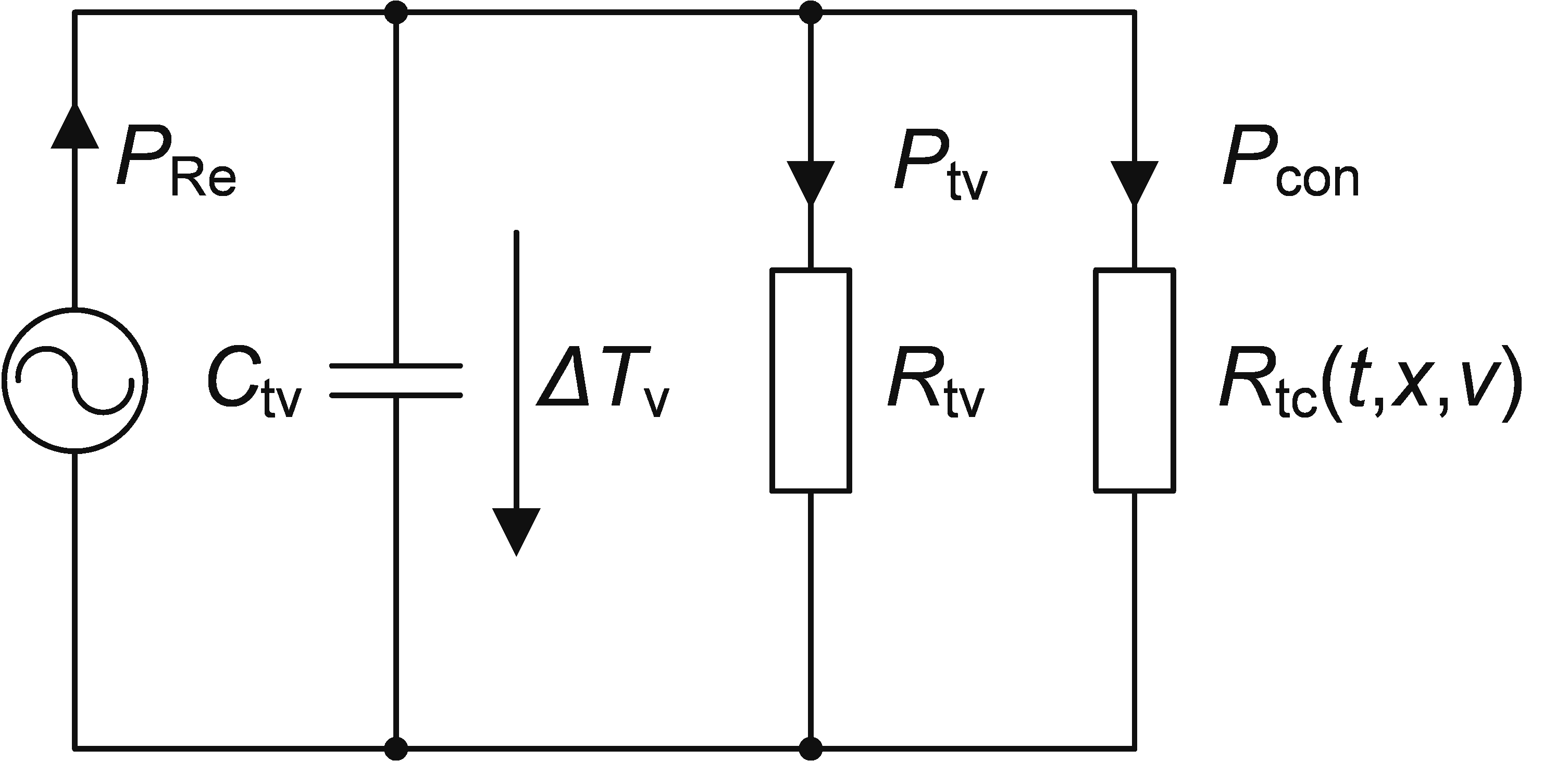
FLSI identifies the parameters of the short-term thermal model displayed below.
Short-term thermal model
A parameter identification algorithm determines the thermal parameters of the transducer:
The thermal capacitance\(C_\mathrm{tv}\) is primarily related to the mass of the voice coil, as it reflects the coil’s ability to store thermal energy.
The thermal resistance\(R_\mathrm{tv}\) is mainly associated with the surface area of the voice coil, which determines the rate of heat dissipation through conduction and radiation.
The effective bypass factor\(\gamma_\mathrm{con,eff}\), which depends on \(R_\mathrm{tv}\) and \(R_\mathrm{tc} (t,x,v)\) for the given stimulus, accounts for convective cooling effects. It depends on the surface area of the voice coil, the voice-coil position, the air velocity in the gap, and the temporal evolution of these quantities.
This model is designed to provide reliable and repeatable results for any type of electro-dynamic transducer within a short measurement time.
This is particularly valuable for:
quickly estimating the voice coil’s power handling capabilities,
experimenting with different voice coil and motor geometries, and different voice coil former materials,
assessing the effect of convection cooling by evaluating the bypass factor \(\gamma_\mathrm{con,eff}\)
Note
The linear parameters of the thermal model, \(C_\mathrm{tv}\) and \(R_\mathrm{tv}\),
are independent of the measurement configuration.
However, to ensure accurate parameter identification, it is essential that the voice coil temperature is approximately
at room temperature at the beginning of the measurement.
This implies that when repeating a measurement (including THERMAL MODE) on the same DUT, a cool-down period may be necessary.
For micro-speakers, a pause of about one minute or less is typically sufficient.
In contrast, for large transducers such as subwoofers, a longer cool-down time of up to 10 minutes may be required.
The temperature state of the voice coil can be verified by running only the LINEAR MODE in FLSI:
if the measured small-signal DC resistance \(R_\mathrm{e}\) is within approx. 2% of the initial value (measured on a cold voice coil),
the full measurement can proceed.
Unlike \(C_\mathrm{tv}\) and \(R_\mathrm{tv}\), convection cooling represented by the bypass factor \(\gamma_\mathrm{con,eff}\)depends on the stimulus — it is influenced by state variables such as voice coil velocity and
displacement, and temporal variations of voice coil movement.
Consequently, comparisons of \(\gamma_\mathrm{con,eff}\) between different DUTs are only meaningful if the stimulus
is comparable across measurements.
This can be ensured, for instance, by manually adjusting the stimulus level in the FLSI property page.
is the difference between the absolute mean voice coil temperature \(T_\mathrm{v}(t)\) and much slower changing
ambient temperature \(T_\mathrm{a}(t)\).
It is approximated using the measured change of the voice coil DC resistance \(R_\mathrm e\).
FLSI uses a fixed temperature coefficient of \(\alpha_\mathrm{T} = 0.0038 \frac{1}{K}\).
Example:
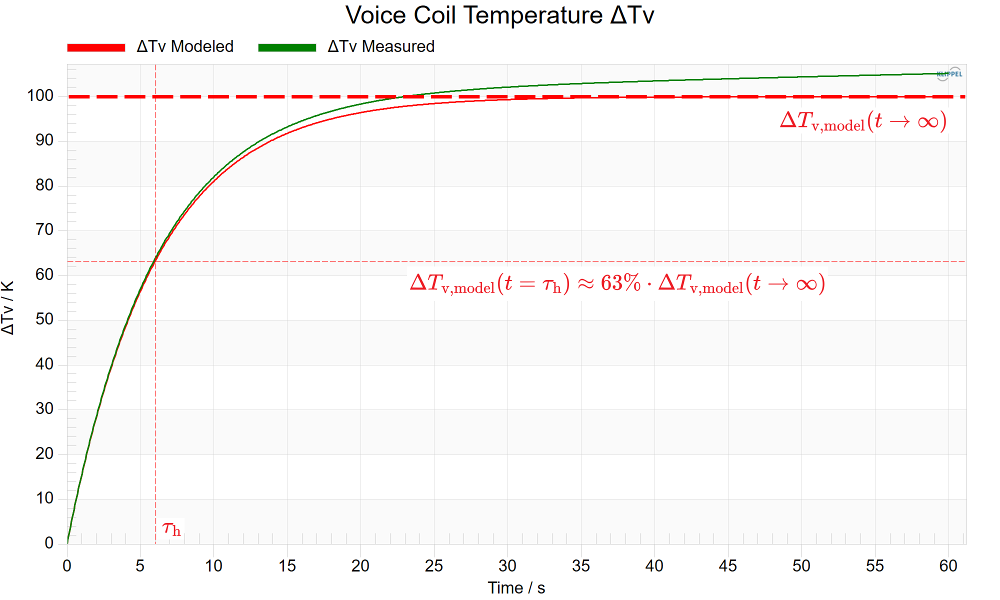
The plot below shows typical measured (green) and simulated (red) voice coil temperature rise of a small woofer over a duration of one minute
under multi-tone excitation at a constant level, assuming negligible convection cooling.
Modeled and measured voice coil temperature
It can be observed that the modeled temperature closely matches the measured temperature at the beginning of the measurement,
up to approximately twice the thermal time constant \(\tau_\mathrm{v}\).
For longer excitation times, simulation and measurement begin to deviate due to the heating of surrounding materials (e.g., iron and magnet),
which is not captured by the short-term thermal model.
This information is useful for estimating the worst-case short-term power handling
capability of the voice coil (neglecting convection cooling), using the relationship
where \(\Delta T_\mathrm{v,max}\) is the maximum permissible voice coil temperature rise, determined by the specifications of the voice coil and the voice coil former.
In addition to power handling, the thermal parameter measurement allows the estimation of convection cooling
by means of the bypass factor
The parameter \(\gamma_\mathrm{con,eff}\) ranges between 0% and 100%.
A larger bypass factor indicates that a greater portion of the heat is directly transferred to the motor structure
and the surrounding environment, rather than contributing to heating of the voice coil.
If \(\gamma_\mathrm{con,eff}\) is close to 100% for a given stimulus, convection cooling is highly effective; if it is close to 0%, its effect is negligible.
Note
The short-term thermal model is not intended for identifying parameters for long-term simulations.
The focus in FLSI is to provide parameters that are repeatable and physically interpretable,
so they can be directly used in the transducer design process or for comparing the thermal behavior of different transducers,
for example in parameter studies.
While more complex thermal models (e.g. Nonlinear Modeling of the Heat Transfer in Loudspeakers)
with multiple thermal nodes can, in principle, represent the system in greater detail and enable prediction of long-term thermal behavior,
their parameters are difficult to identify reliably.
In practice, such models suffer from non-uniqueness in the parameter fitting process,
meaning that different parameter sets can produce similarly good fits to the measured data.
As a result, the identified parameters may show limited repeatability across measurements, which complicates their physical interpretation.
The following loudspeaker system types are currently supported and can be selected on the FLSI property page.
Note that the lumped parameter models shown below are simplified linear representations.
Additional effects identified by FLSI — such as leakage losses and mechanical creep —
are included in the parameter estimation but are not explicitly shown in these models.
Free Air
An electrodynamic transducer without enclosure.
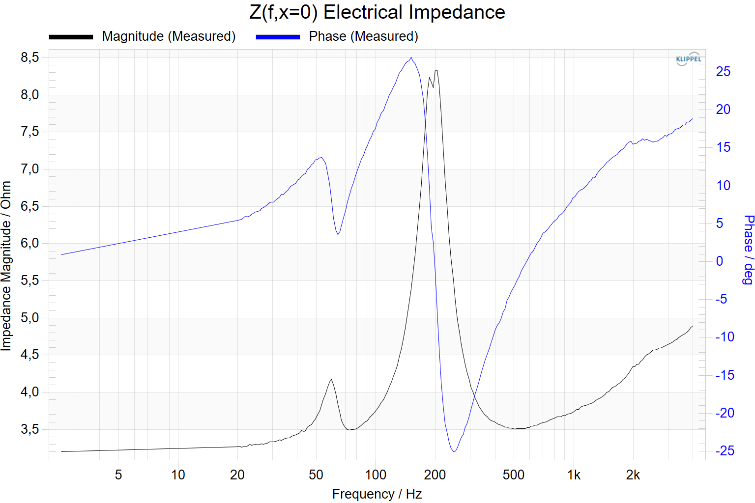
The mechanical system is described by a second-order system (one distinct resonance peak in the electrical impedance magnitude).
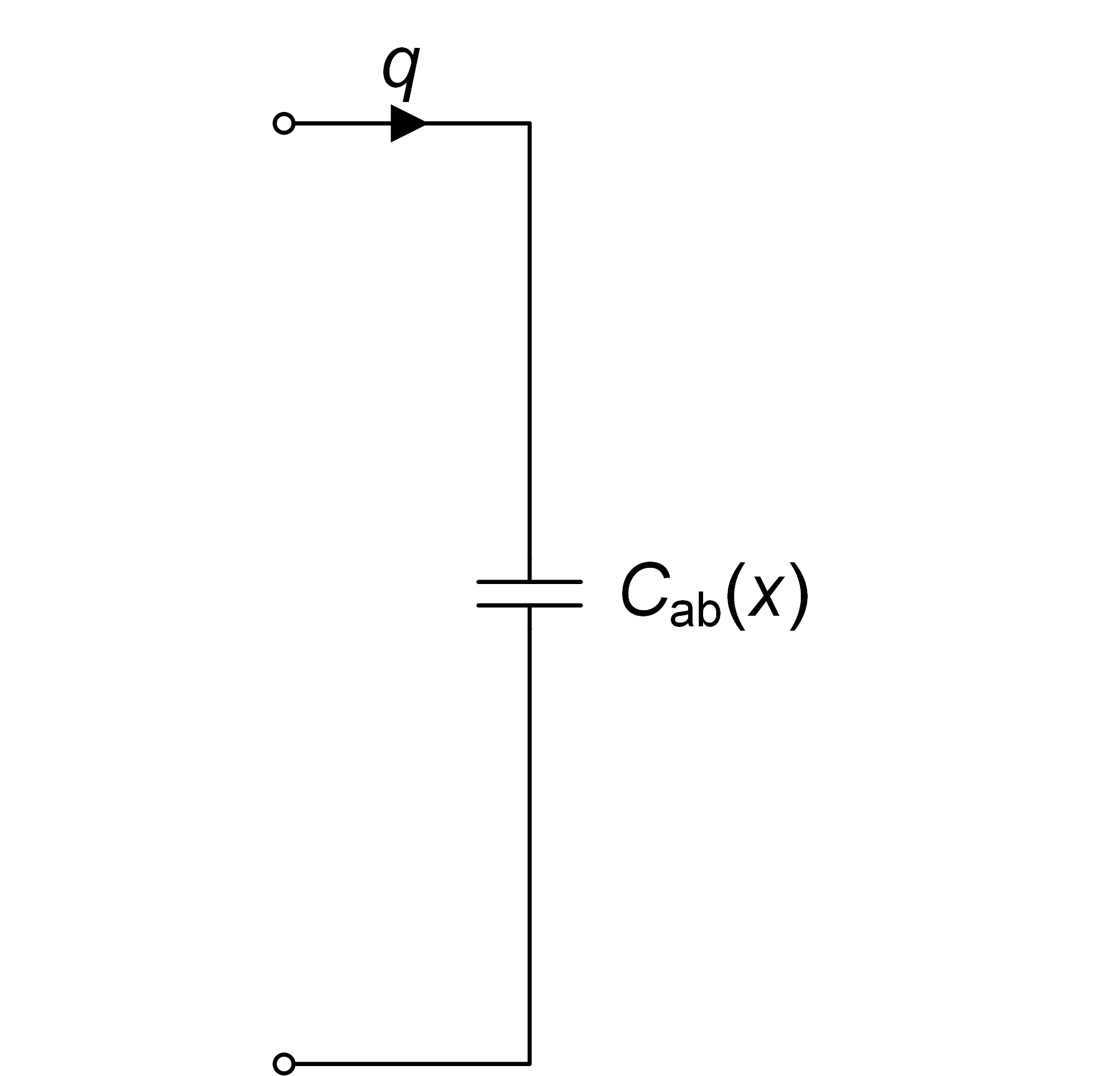
Closed box
An electrodynamic transducer mounted in a closed enclosure.
The mechanical system is described by a second-order system (one distinct resonance peak in the electrical impedance magnitude).
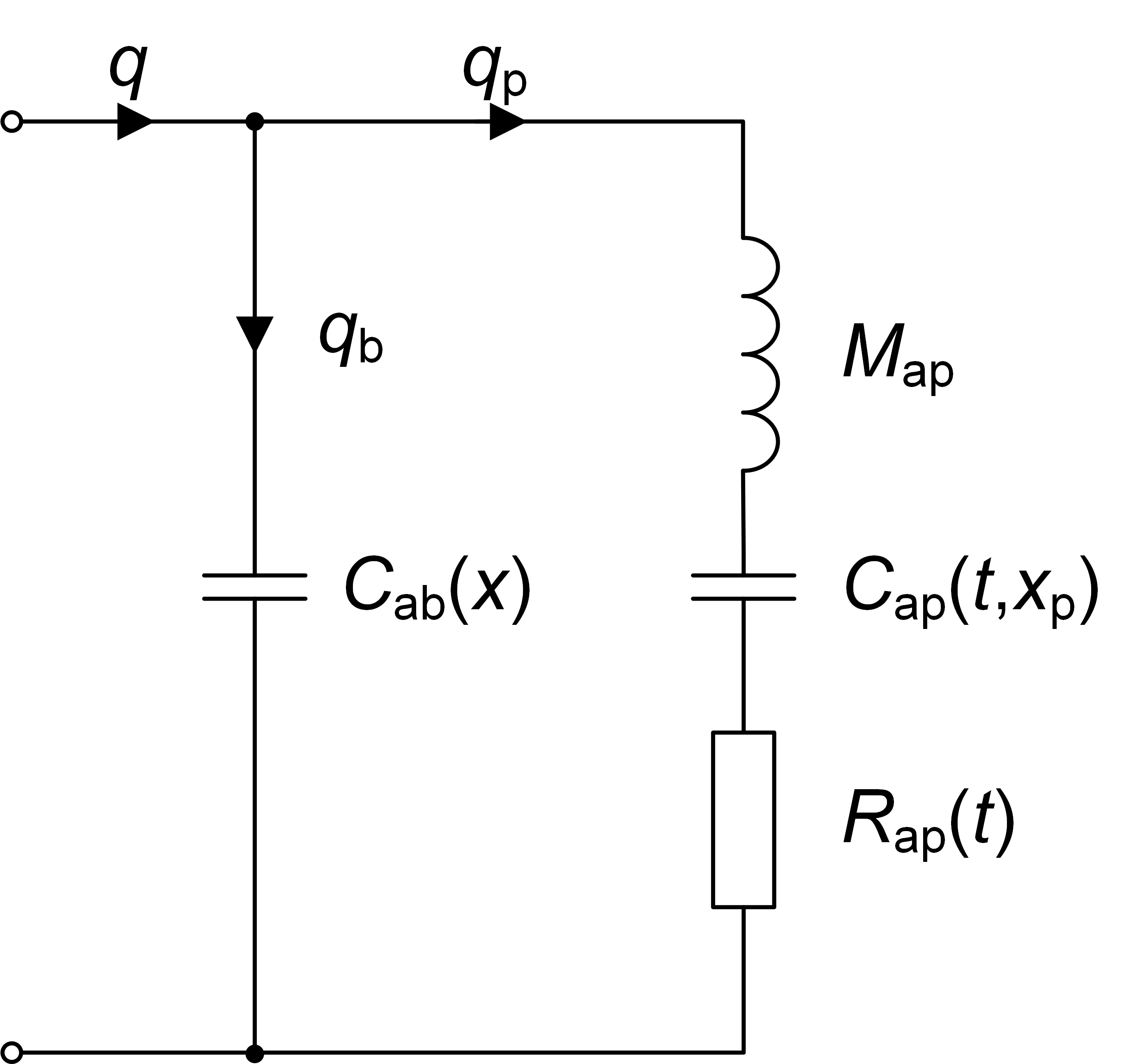
The compliance \(C_\mathrm{ab}(x)\) represents the compliance of the enclosed air in the rear chamber.
The chamber volume is modulated by the cone displacement, resulting in a nonlinear air compliance.
A small barometric vent is usually included to equalize atmospheric pressure.
The corresponding resistance is not explicitly shown in the model below.
Closed box model
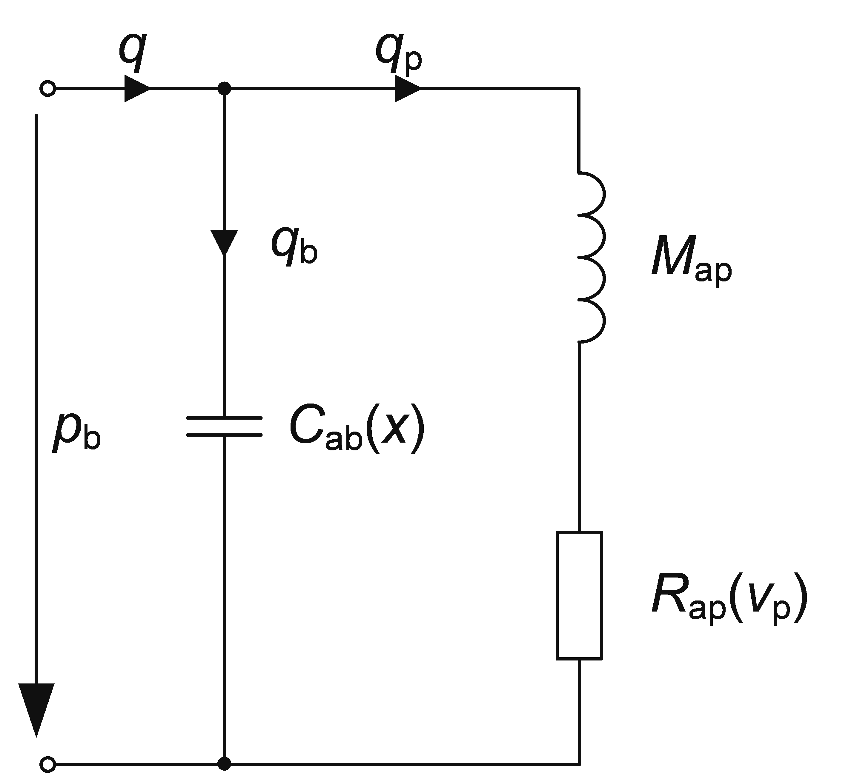
Vented box
Also referred to as bass reflex system.
An electrodynamic transducer mounted in an enclosure with an opening (e.g., a port or pipe).
Together, they form a Helmholtz resonator excited by the transducer.
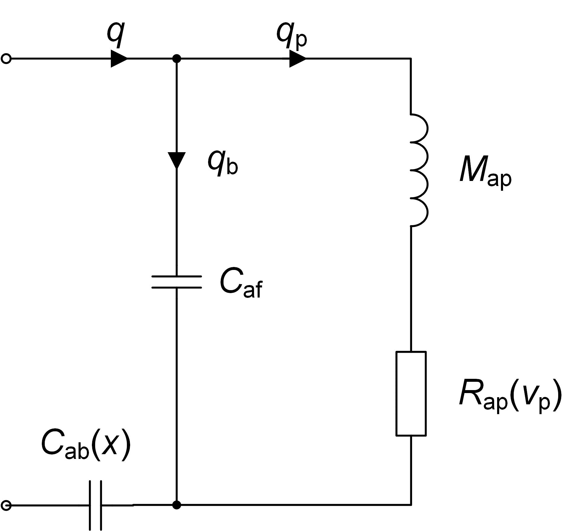
The mechanical system is described by a fourth-order system (two distinct resonance peaks in the electrical impedance magnitude).
At higher excitation levels, air particle velocities in and around the port can become very high.
This leads to increased acoustic losses due to vortex shedding as well as laminar and turbulent flow resistance, which can generate significant nonlinear distortion.
In addition, an asymmetric nonlinear port resistance (see Nonlinear Parameters)
may cause a significant DC displacement of the voice coil.
Vented box model
Passive radiator
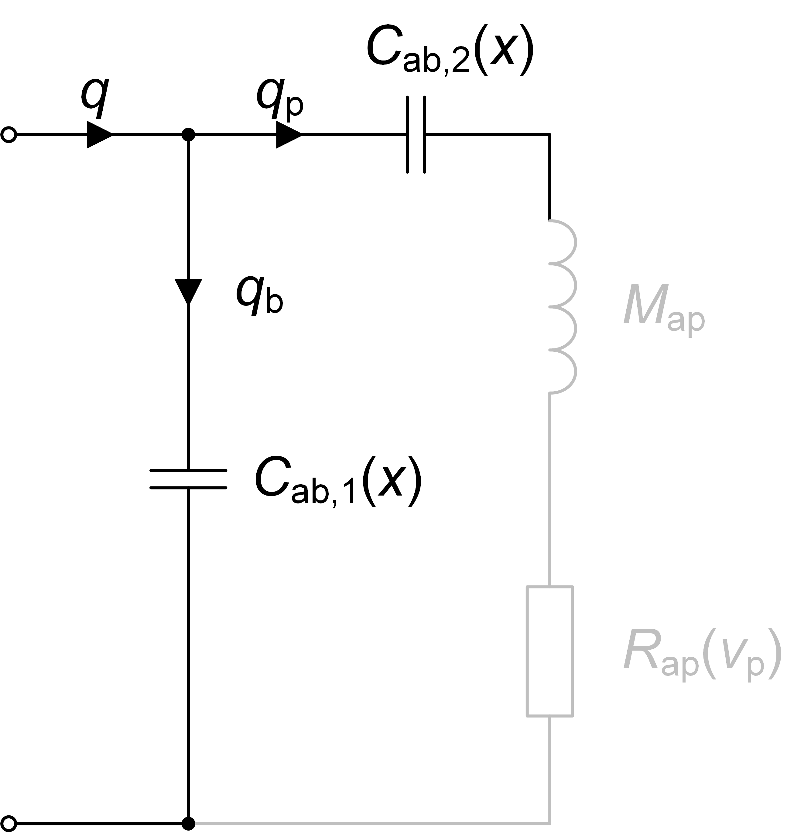
An electrodynamic transducer mounted in an enclosure drives a passive membrane (spring–mass system) within the same enclosure.
The mechanical system is described by a fourth-order system (two distinct resonance peaks in the electrical impedance magnitude).
Similar to the nonlinear suspension of the active transducer (see Mechanical Resonator),
the passive radiator’s stiffness and damping are nonlinear and time-variant, depending on displacement and operating conditions.
Passive radiator model
Sidefire
A small electrodynamic transducer mounted in an enclosure that is closed at the rear side of the diaphragm and features a small sound outlet on the front side.
Such configurations are commonly used in mobile devices.
The linear model of this system corresponds to a fourth-order bandpass system, typically exhibiting two resonance peaks in the electrical impedance magnitude.
If only a single distinct resonance peak is observed, the system may be described as a second-order system.
Sidefire speaker model
Tweeter
An electrodynamic transducer designed for high-frequency reproduction.
Typically, the voice coil is directly attached to a dome-shaped diaphragm.
This assembly operates against a closed rear cavity, which may include a small internal vent.
The mechanical system can be described by either a second-order or fourth-order system (one or two resonance peaks in the electrical impedance magnitude).
The appropriate model order is determined automatically by the fitting algorithm.
If the rear volume is not sealed, select Free Air or Vented Box instead.
Tweeter model
Moving-Magnet Transducer
A moving-magnet transducer uses a fixed coil and a magnet as the moving element.
This principle is commonly used in exciters, but is also found in certain subwoofer designs.
The modeling of moving-magnet transducers is largely similar to that of moving coil transducers.
However, several important differences must be considered:
The electro-mechanical coupling cannot be described by the force factor \(Bl(x)\), but instead by the electro-mechanical transduction factor \(T_\mathrm{em}(x)\)
The mechanical stiffness \(K_\mathrm{ms}(t,x)\) consists of both a mechanical component (suspension) and a magnetic suspension component
The mechanical damping \(R_\mathrm{ms}\) includes not only mechanical losses, but may also contain iron losses
The reluctance force, as defined in Self-Inductance, does not occur in moving-magnet transducers
FLSI determines loudspeaker parameters in the electrical domain from the measured voltage and current signals
(see simplified linear model in the electrical domain below).
Simple linear transducer model in the electrical domain
To derive the actual mechanical parameters — such as moving mass and mechanical stiffness — according to the full
nonlinear loudspeaker model, a calibration factor is required.
This calibration links the electrical model to the mechanical domain and is typically based on the force factor
\(Bl(x=0)\) or an equivalent mechanical reference parameter.
It is strongly recommended to allow FLSI to perform mechanical calibration automatically using a laser.
This provides the most accurate and robust results.
However, in situations where optical access is not available, mechanical calibration can be performed manually by specifying either:
\(M_\mathrm{ms}\) (moving mass), or
\(Bl_\mathrm{max}\) (maximum force factor over displacement), or
\(Bl(x=0)\) (force factor at rest position)
The parameter \(Bl_\mathrm{max}\) refers to the peak value of the \(Bl(x)\) curve across the full displacement range,
rather than only at the rest position (\(x = 0\)).
Note
If manual calibration is required, the calibration parameter value should be obtained from a separate FLSI measurement where laser access is available,
e.g., by measuring the transducer in free air or with the grill removed.
Use \(M_\mathrm{ms}\) import whenever the acoustical environment remains unchanged between the reference measurement and the measurement without laser access. This usually provides the most robust and consistent calibration.
Use \(Bl_\mathrm{max}\) import if the acoustical environment changes (e.g., due to waveguides, grills made of dense materials, or vacuum measurements).
Detailed Explanation:
In most cases, the use of the moving mass\(M_\mathrm{ms}\)is recommended for mechanical calibration,
because calibration based on \(Bl(x=0)\) is more sensitive to small identification errors.
This is because the parameter identification is performed in the electrical domain, where the moving mass transformed into the electrical domain, \(C_\mathrm{mes}\), is identified.
The moving mass is then calculated using \(M_\mathrm{ms} = C_\mathrm{mes} Bl(x=0)^2\).
Consequently, small errors in \(Bl(x=0)\) lead to a quadratic error contribution in the estimated \(M_\mathrm{ms}\).
In addition, the moving mass is typically the most stable parameter between the small- and large-signal domains.
By contrast, \(Bl(x=0)\) may vary due to magnet temperature fluctuations, particularly in small transducers using neodymium magnets.
As a result, moving mass import generally provides the most consistent parameter set between the small- and large-signal domains.
However, if the acoustical environment of the transducer changes between the reference measurement with laser and the measurement without laser,
the moving mass may change, because this comprises the moving air in front of the transducer’s membrane.
Also, do not apply moving mass calibration of a measurement in air in a vacuum measurement, and vice versa,
as the moving mass will be different due to the lack of air in the vacuum measurement.
If the acoustical environment changes due to waveguide or a dense grill, the mass cannot be assumed to be constant and a \(Bl\) import is preferred.
In this case, it is highly recommended to use \(Bl_\mathrm{max}\) instead of \(Bl(x=0)\) as mechanical calibration parameter.
This is because the rest position may shift during large-signal operation (commonly observed when drivers are mounted in relatively small enclosures),
causing \(Bl(x=0)\) not to be constant between different measurements under any circumstances.
Instead of the automatic mechanical calibration or specifying
a \(Bl(x=0)\) or moving mass value manually, the Added Mass Method can be performed.
Usually it is recommended to use a laser for the mechanical calibration.
However, in some cases the added mass method is preferable, e.g.
if no laser is available
if the laser cannot be used due to bad optical conditions
validating the mechanical calibration using different measurement techniques
training and academic purposes
The added-mass method should be performed using the following procedure:
Create a new FLSI operation.
Apply an additional mass to the transducer’s cone, e.g. clay. Its mass should roughly be in the range of roughly 40-100 % of the estimated transducer’s moving mass.
Open the FLSI operation’s property page.
Configure the measurement (Speaker System Type, Limits, …)
In the Mechanical Calibration drop-down list, select Added Mass Method.
Press the button Create Operation for Added Mass Measurement. This creates a new operation which will be used to perform a small signal measurement with an additional mass applied to the transducer’s moving mass.
Run the newly created FLSI operation Measurement with Added Mass
Remove the moving mass.
Open the property page of the FLSI operation that you have created in step 1.
Press the button Import Measurement with Added Mass and select the FLSI operation Measurement with Added Mass of step 4.
Insert the precise value of the added mass in the Added Mass input field.
Entering geometry data of driver and enclosure is optional. If the effective radiation area \(S_\mathrm{d}(x=0)\) or the corresponding diameter is provided,
additional derived linear parameters, such as \(V_\mathrm{as}\), are calculated and displayed in the linear parameter result table.
The effective radiation area can be measured accurately using SCN – Scanning Vibrometer.
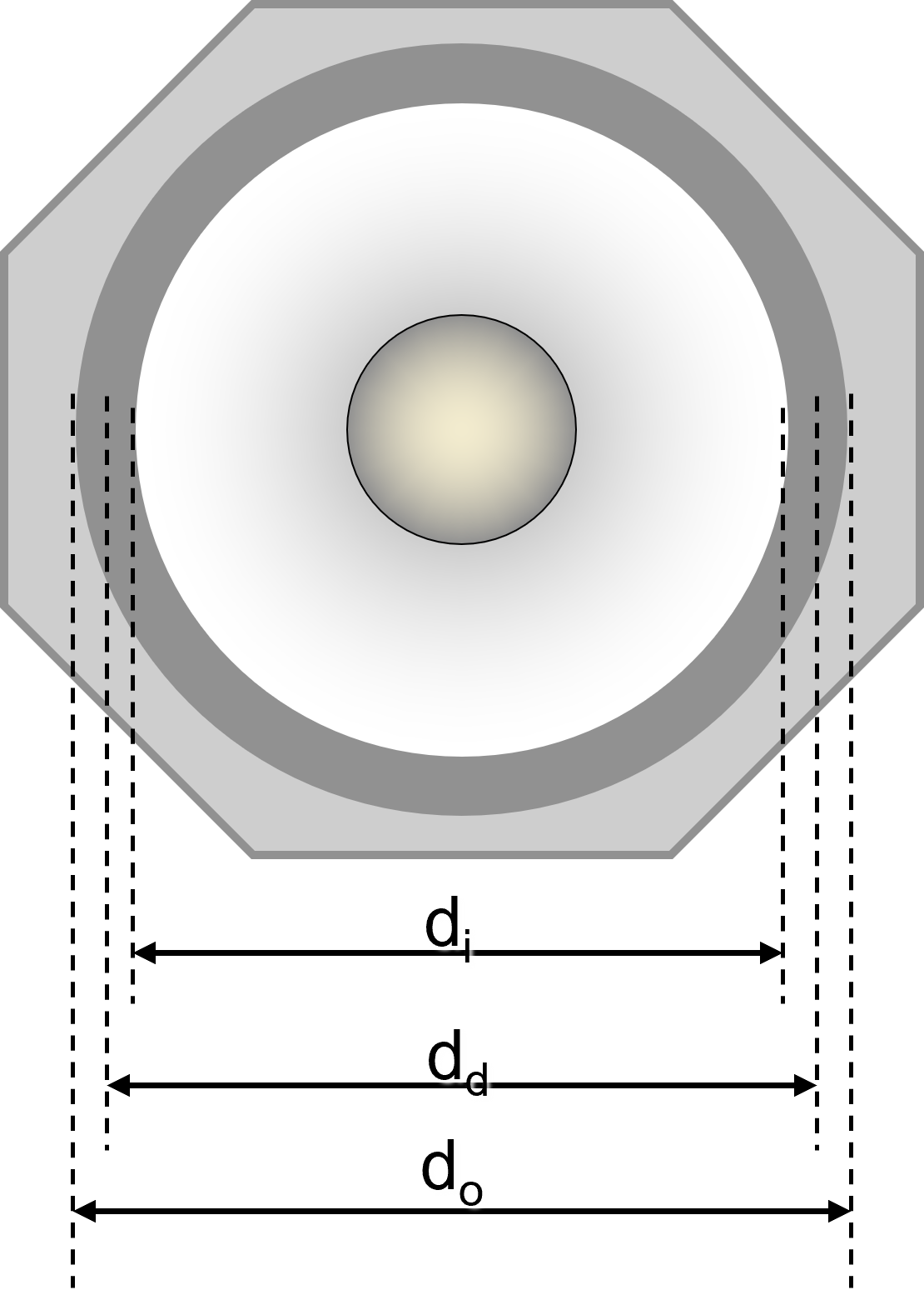
If this is not possible, \(S_\mathrm{d}(x=0)\) for circular drivers can be approximated using the effective diameter:
When using this approximation, slightly higher tolerances should be expected for derived parameters that depend on \(S_\mathrm{d}(x=0)\).
Do not use the nominal driver diameter (e.g., 4” or 5.25”), as it does not represent the effective radiating area.
The calibration parameters are post-processing parameters that can be changed after the measurement.
Small-Signal vs. Linear Parameters at the Rest Position#
Linear parameters are required as input for traditional loudspeaker modeling.
In this context, they are assumed to be constant and independent of the excitation,
meaning that any dependence on state variables such as displacement \(x\) or voice coil temperature \(T_\mathrm{v}\) is neglected.
This assumption is valid only in the small-signal domain, where the transducer operates at very low amplitudes and behaves approximately linearly.
Time-variant effects, such as creep and thermal dynamics (see Mechanical Resonator)
As a result, the parameters of the transducer vary with time and operating conditions.
This leads to systematic differences between parameters derived in the small-signal domain and those observed under large-signal conditions.
More information can be found in section Large-Signal Modeling.
To maintain compatibility with traditional linear models while reflecting realistic operating conditions,
linear parameters in FLSI are defined at the rest position (x = 0) under large-signal excitation.
Small-signal parameters
Measured at very low amplitudes
Represent an idealized, purely linear system
Linear parameters at x = 0
Derived under realistic large-signal excitation
Include the influence of thermal and time-variant effects
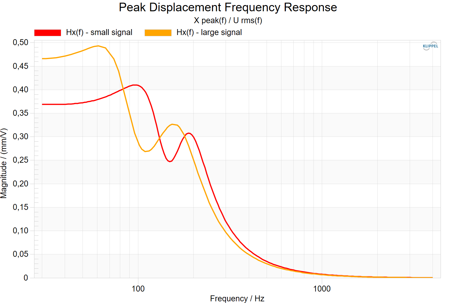
The \(H_\mathrm{x,peak}(f)\) chart below shows the peak displacement versus excitation voltage of a vented-box system,
using both small-signal parameters and large-signal parameters at the rest position.
The two curves show significant deviations, caused by the time-variant behavior of the transducer.
To accurately simulate the loudspeaker’s behavior, it is therefore necessary to consider linear parameters, nonlinear parameters, and time-variant effects.
At the same time, linear parameters such as resonance frequencies, Q-factors, and sensitivity remain easy-to-interpret quantities
and continue to provide valuable insight for engineering and communication, i.e. the alignment of transducer and enclosure.
In addition, identifying time-variant behavior provides important benefits for the loudspeaker and transducer engineer, for example:
Revealing design weaknesses, such as limited robustness
Estimating thermal compression effects under realistic operating conditions
Quantifying dynamic shifts of the operating point (e.g., DC displacement)
The table Linear Parameter at x=0 table displays the parameters of the
lumped parameter model in the small signal domain
and in the large signal domain at the voice coil rest position x=0.
If the Nonlinear Mode is activated on the FLSI’s property page, three columns are displayed:
LARGE+WARM (large signal domain + warm speaker)
measured in the NONLINEAR MODE
the peak voice coil displacement is high: \(|x_\mathrm{peak}| \ll x_\mathrm{prot}\),
the variation of the parameters is not negligible: \(C_\mathrm{min} \ll 100\%\) and/or \(Bl_\mathrm{min} \ll 100\%\),
the voice coil temperature might be increased (\(\Delta T_\mathrm{v} > 0\)) due to heating.
LARGE+COLD (large signal domain + cold speaker)
measured in the LINEAR and NONLINEAR MODE
the peak voice coil displacement is high: \(|x_\mathrm{peak}| \ll x_\mathrm{prot}\),
the variation of the parameters is not negligible: \(C_\mathrm{min} \ll 100\%\) and/or \(Bl_\mathrm{min} \ll 100\%\),
the effect of heating is compensated while considering the cold voice coil resistance measured in the LINEAR MODE where \(\Delta T_\mathrm{v} \approx 0\).
SMALL SIGNAL (small signal domain + cold speaker)
measured in the LINEAR MODE
the amplitude of the excitation signal is small,
the displacement is small in comparison to the allowed maximum displacement: \(|x_\mathrm{peak}| \ll x_\mathrm{prot}\),
the variations of the nonlinear parameters are negligible: \(C_\mathrm{min} \approx 100\%\) and/or \(Bl_\mathrm{min} \approx 100\%\),
the increase of voice coil temperature is negligible: \(\Delta T_\mathrm{v} \approx 0\),
the effects of the nonlinear, thermal and time-varying mechanisms are negligible and the transducer behaves almost linear.
Section Self-Inductance introduced the linear inductance impedance \(Z_\mathrm{L}(f, x=0, i=0)\)
as a frequency-dependent electrical lumped element.
While this representation is well suited for analysis, it is not directly compatible with most simulation tools
(such as SIM), which typically require an equivalent circuit model.
For this reason, the parameters of the linear LR-3 inductance model are provided here for export and use in such tools.
In addition, the clipboard export (property page \(\rightarrow\) Im/Export) provides access to the nonlinear LR-3 model parameters:
\(L_\mathrm{e}(x)\), \(L_\mathrm{2}(x)\), \(R_\mathrm{2}(x)\), \(L_\mathrm{3}(x)\), and \(R_\mathrm{3}(x)\).
Linear inductance model
Note
The LR-3 inductance model parameters are valuable as input for simulation tools.
However, they are not physically interpretable and cannot be directly compared between different transducers.
For this reason, it is recommended to compare the frequency-dependent impedance curves \(Z_\mathrm{L}(f,x)\) instead,
which provide a physically meaningful basis for comparison.
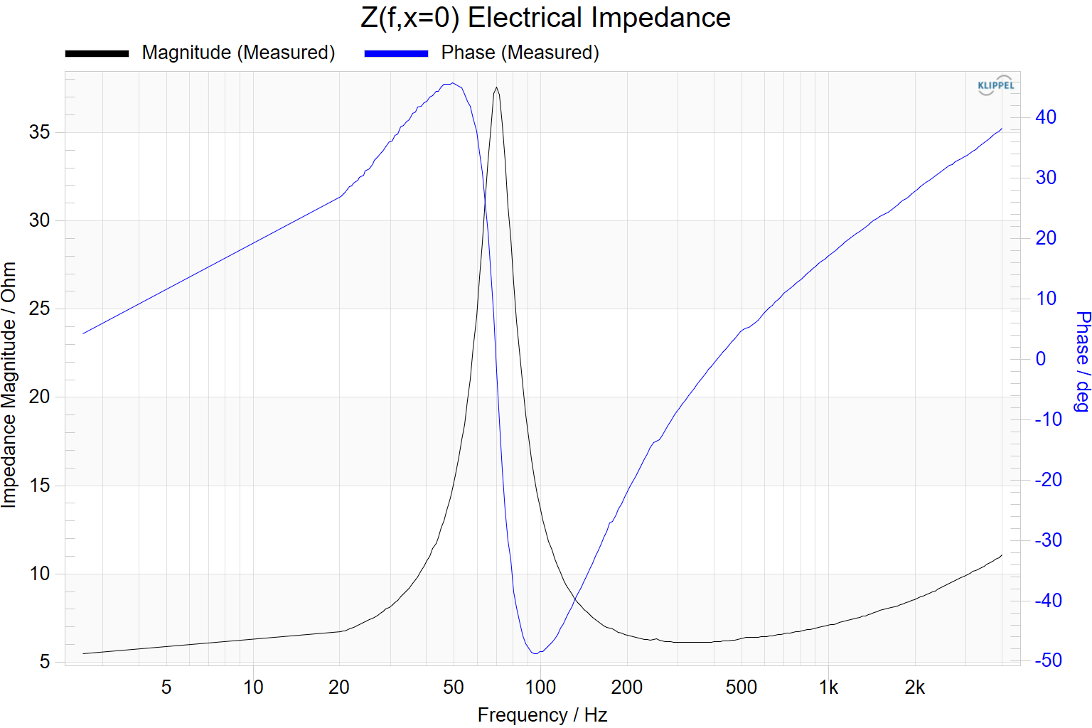
The complex electrical impedance is the transfer function between voltage and current
\[Z_\mathrm{e}(f) = \frac{U(f)}{I(f)}.\]
This transfer function can both be measured and calculated using the identified linear parameters.
The FLSI’s electrical impedance result window displays the magnitude and the phase
(right-click in the window and activate Show All Curves) of the following
impedances:
Magnitude / Phase (measured)
measured impedance in the small signal domain (LINEAR MODE)
Magnitude / Phase (fitted)
fitted impedance that is calculated based on the parameters identified in the small signal domain (LINEAR MODE)
includes mechanical creep
Magnitude / Phase (Thiele-Small simplification)
fitted impedance that is calculated based on the parameters identified in the small signal domain (LINEAR MODE)
\[\underline{Z_\mathrm{L}}(f) = 2\pi f j L(f) + R_\mathrm{L}(f).\]
The latter representation can be easier to interpret than the magnitude and phase.
For instance, the losses that are transformed into heat can be seen directly
for each frequency and compared to the DC resistance Re.
The linear transfer function between the voice coil displacement \(X(f)\)
and the excitation voltage \(U(f)\)
\[H_{\textrm{x}}(f) = \frac{X(f)}{U(f)}\]
can be measured
with a laser or calculated using the identified linear parameters like resonance frequency, Q-factors
and the force factor.
The two transfer functions should be almost identical.
If not, the laser measurement might have been disturbed or the model was not identified with sufficient accuracy.
The transfer functions can be calculated in both the small signal (LINEAR MODE) and the large signal (NONLINEAR MODE)
measurement.
Calculating the laser displacement transfer function in the small signal domain is relatively simple, because the laser and voltage
signals can be divided in the frequency-domain without any further processing.
However in the large signal domain, the processing is more complex because linear transfer functions
are only defined for linear signals.
Hence, the nonlinear distortion which was identified in the parameter identification algorithm
is removed from the measured nonlinear laser signal before calculating the transfer function.
The peak displacement frequency response is calculated by multiplying this transfer function
by the crest factor of a sinus tone \(\sqrt 2\).
This peak displacement frequency response is highly valuable for estimating how much peak displacement can be reached with
a sinus tone of a certain RMS voltage.
The peak displacement produced by a 1 VRMS sinus tone can be directly read from this curve.
Note that this estimation is purely linear and does not consider nonlinear distortion.
The following displacement frequency response magnitudes are displayed:
Laser (small signal)
measured \(|H_{\textrm{x,peak}}(f)|\) in the small signal domain (LINEAR MODE)
Fitted (small signal)
fitted \(|H_{\textrm{x,peak}}(f)|\) that is calculated based on the parameters identified in the small signal domain (LINEAR MODE)
includes mechanical creep
Thiele-Small (small signal)
fitted \(|H_{\textrm{x,peak}}(f)|\) that is calculated based on the parameters identified in the small signal domain (LINEAR MODE)
This result window shows the voltage sensitivity of the transducer as a function of frequency, referenced to 1 m distance, 1 V input, and half-space radiation (2π).
\(S_\mathrm{d}\) import is required for displaying the following curves:
Modeled (small-signal)
Calculated using the linear parameter set. This curve represents the idealized response under low-level excitation, assuming constant parameters.
Modeled (large-signal, warm)
Calculated using the linear parameters at the rest position derived under large-signal conditions.
This curve reflects the influence of thermal and time-variant effects, providing a more realistic estimate of sensitivity under typical operating conditions.
Modeled (large-signal, cold)
Calculated using the linear parameters at the rest position derived under large-signal conditions, but with the small-signal (cold) DC resistance.
This curve reflects the influence of time-variant effects without thermal compression, providing an estimate of sensitivity
under large-signal conditions at low average power (i.e., stimuli with high crest factor).
Measured (laser, small-signal)
Derived from the cone displacement measured by the laser in LINEAR MODE, assuming piston-like radiation.
The displacement signal is differentiated twice to obtain acceleration, which is then converted into radiated sound pressure under the 2π assumption.
Accurate results require proper laser alignment and valid mechanical calibration.
The measured curve provides a direct reference to the physical response and can reveal deviations from the modeled behavior.
Differences between small- and large-signal curves indicate the impact of time-variant effects, in particular thermal compression and time-variant mechanical suspension behavior (stiffness and damping).
Note that sensitivity curves are currently not available for passive radiator and moving-magnet transducers.
Note
Sensitivity curves may slightly differ from curves obtained by simulation tools, such as LSIM, as FLSI considers creep
and leakage losses in speaker systems with closed rear chamber.
FLSI identifies parameters by minimizing the error between measured and simulated states (primarily the electric current).
If a parameter, such as \(Bl(x)\) or \(K_\mathrm{ms}(x)\), has little or no influence on the states,
the sensitivity of parameter fitting is low.
This means that:
The parameter has negligible influence on the loudspeaker’s behavior and performance.
The parameter should not be interpreted further — it generally does not contain relevant information.
The shape of the nonlinear parameter may be imprecise because no useful information could be extracted from the underlying states.
To check whether a parameter is relevant for the device’s behavior, review:
Distortion Components in Large Signal Characteristics (Single Values):
If the distortion component’s value is very small (less than 1 %), the parameter is usually negligible.
In this case, the distortion component value is displayed in light gray.
Displacement Limits:
If the displacement limit is greater than the maximum displacement reached during the measurement, the parameter may be irrelevant.
Confirm by also checking the distortion components.
Note that a parameter that is irrelevant in one measurement can be important in another with different conditions:
Increasing the excitation voltage can generate more distortion, making a parameter more significant.
Mounting the transducer in an enclosure can make parameters important that were negligible in a free-air measurement due to different operating conditions (e.g., higher stiffness and current).
In all nonlinear parameter curves that depend on displacement \(x\), a solid black vertical line is shown.
This line represents the instantaneous rest position of the voice coil.
If a laser is used, the measured rest position — the position the coil would return to if the stimulus
were turned off — is displayed as a dotted vertical line.
A deviation between the dotted and solid lines indicates that one of the following conditions may be present:
The voice coil rest position has shifted during the large-signal measurement.
This can occur if the suspension changes its geometry during the test.
Such a shift is usually an undesired defect.
An unmodeled DC force is present.
This effect is sometimes observed in small, closed enclosures:
Closed boxes are never perfectly sealed;
they must include a barometric vent to equalize pressure between the enclosure’s interior and the surrounding air.
In such cases, a DC force — often caused by a nonlinearity like the reluctance force — acts not on the total stiffness
(\(K_\mathrm{mt}\)), but primarily on the mechanical stiffness (\(K_\mathrm{ms}\)).
As a result, the DC force acting only on \(K_\mathrm{ms}\)
causes a larger DC displacement than if it acted on \(K_\mathrm{mt}\) (the stiffness determined by the parameter identification).
In this case, the parameter identification algorithm may underestimate the actual DC displacement
which results in a shifted instantaneous rest position.
The laser or DUT is not in a fixed position.
This is a measurement setup error and should be corrected.
The force factor \(Bl(x)\), also called electrodynamic coupling factor or
electromechanical transduction factor, is
defined by the integral of the magnetic flux density \(B\) over voice coil length \(l\).
The solid gray curve \(Bl(-x)\) represents the force factor mirrored at the rest position.
This visualization helps to identify any asymmetries in the suspension.
This parameter is only available in moving-magnet transducers.
\(T_\mathrm{em}(x)\) is electro-mechanical transduction factor linking electrical with mechanical domain.
Its distortion symptoms (compression, harmonic, intermodulation distortion) are very similar to \(Bl(x)\).
The stiffness \(K_\mathrm{ms}(x)\) characterizes the mechanical properties of the suspension and is the
inverse of the compliance \(C_\mathrm{ms}(x)\).
The nonlinear stiffness is defined as the secant stiffness of the lossless restoring force–deflection curve
characteristic \(F(x)\):
where \(x_0 = 0\) denotes the voice-coil rest position.
The solid gray curve \(K_\mathrm{ms}(-x)\) represents the stiffness mirrored at the rest position.
This visualization helps to identify any asymmetries in the suspension.
If the speaker’s enclosure is closed, the chart displays the total stiffness of the system:
In order to display the driver stiffness \(K_\mathrm{ms}(x)\) and the stiffness of the enclosed air
\(K_\mathrm{mb}(x)\), it is necessary to specify \(S_\mathrm{d}(x=0)\) and the box volume \(V_\mathrm{b}\)
on the property page (see Acoustical Calibration (Geometry)).
The parameters \(S_\mathrm{d}(x=0)\) and \(V_\mathrm{b}\) can be changed after the measurement is complete.
The enclosure type must be set before the measurement, though.
The small-signal stiffness, measured in the LINEAR MODE, is displayed alongside the nonlinear stiffness,
measured at high amplitude during the NONLINEAR MODE.
This allows for a direct comparison of how the mechanical stiffness changes at the rest position across different levels.
In moving-magnet transducers, the stiffness \(K_\mathrm{ms}(x)\) comprises both mechanical (e.g., spider) and
magnetic stiffness.
FLSI also calculates the incremental (small-signal) stiffness, which can be accessed by right-clicking in
the \(K_\mathrm{m}(x)\) window and selecting Show All Curves.
The incremental stiffness is defined as the local derivative of the restoring force with respect to displacement:
where \(x_k\) denotes discrete static voice-coil positions at which the stiffness is evaluated.
This curve is particularly useful for comparison with point-by-point measurements or simulations
(see IEC 62458 and
Validating Nonlinear Transducer Motor Simulations with Measurements):
in this approach, the voice coil is moved to positions \(x_k\), and the stiffness is either calculated or measured,
yielding the incremental stiffness \(K_\mathrm{incr}\) over \(x_k\).
Note
The nonlinear compliance curves \(C_\mathrm{ms}(x)\) and \(K_\mathrm{mt}(x)\) can be accessed by right-clicking in the
\(K_\mathrm{m}(x)\) window and selecting Show All Curves.
Viewing these curves can be useful for understanding the protection system, as the protection limit \(C_\mathrm{min}\) refers to the nonlinear compliance.
As described in Self-Inductance, the voice coil’s self-inductance depends on frequency, displacement, and current:
\[\underline{Z}_\mathrm{L}(f,x,i) = 2\pi f j L(f,x,i) + R_\mathrm{L}(f,x,i).\]
Accurately modeling all electro-dynamic effects for real audio signals over a wide bandwidth requires a complex nonlinear dynamic model,
because frequency, displacement, and current are interdependent in a non-trivial way.
However, the results of such a model cannot easily be visualized for intuitive interpretation.
To make the displacement-dependency of inductance interpretable, the model is simplified to a set of blocked impedances:
considering only the DC part of the total displacement which comprises a DC and an AC part:
\[x = x_\mathrm{DC} + x_\mathrm{AC}.\]
The electric current flow (current dependency is covered in Flux Modulation) is assumed to be negligible for
displacement-dependency investigations.
The blocked impedance representation is comparable to the results of a semi-static point-by-point measurement
(see IEC 62458 or Measuring the Nonlinear, Lossy, Frequency-dependent Voice Coil Inductance),
where the voice coil is rigidly fixed at different positions \(x_\mathrm{DC}\),
and small-signal measurements are performed to obtain the electrical impedance curves at these positions.
For simplicity, FLSI’s user interface omits the index \(DC\) and does not explicitly indicate \(i\approx 0\):
In Klippel’s previous large-signal identification software (LSI2 and LSI3), inductance variation was displayed using
a pure inductance \(L_\mathrm{e}(x)\) (also see FAQ, explaining differences between LSI and FLSI).
A more insightful representation is to evaluate the impedance magnitude of the inductance
\(|\underline{Z}_\mathrm{L}(f,x)|,\) calculated at selected frequencies \(f\).
This directly shows how impedance changes with displacement and frequency,
and relates directly to the amplitude modulation produced by inductance nonlinearity.
For example, a large variation in impedance magnitude produces greater amplitude modulation than a small variation.
The pure inductance \(L(f,x)\) shows only part of the distortion mechanism.
Inductance nonlinearity causes both amplitude and phase modulation — with the phase component having much less perceptual impact on audible intermodulation distortion
(further reading: Psychoacoustics - Facts and Models).
In most drivers, inductance exhibits a strongly asymmetric characteristic at low frequencies:
When the voice coil moves toward the back plate, inductance typically increases because the magnetic field generated by the coil encounters lower magnetic reluctance
due to the high permeability of iron.
This property can be used to verify loudspeaker polarity and interpret the excursion direction in diagrams of nonlinear parameters.
The shape of the nonlinearity (symmetric vs. asymmetric) also provides insight into the type of nonlinear distortion:
Asymmetric behavior typically produces second-order distortion intermodulation distortion.
\(|\underline{Z}_\mathrm{L}(f,x)|\) should not be interpreted without considering the voice coil’s DC resistance \(R_\mathrm{e}\), which is also shown in the chart.
If \(|\underline{Z}_\mathrm{L}(f,x)|\) is significantly smaller than \(R_\mathrm{e}\) — as is often the case in micro-speakers and woofers at low frequencies — the distortion caused by self-inductance is usually negligible.
Another useful representation of lossy inductance, showing its dependency on frequency and voice coil position,
is obtained by calculating the ratio between the AC flux linkage\(\Lambda_\mathrm{AC}(f,x)\)
(Fourier-transformed flux linkage \(\lambda_\mathrm{AC}(t,x)\)) and the corresponding electric current \(I(f)\):
Here, the lossy inductance \(L_\mathrm{l}(f,x)\) (in henries) can be interpreted as an inductance derived from the impedance magnitude —
it ignores the phase of \(\underline{Z}_\mathrm{L}\) and treats all impedance as purely inductive.
This quantity is displayed as a color map (contour plot) showing the AC flux linkage distribution
for different voice coil positions (vertical axis) and frequencies (horizontal axis).
Note
While the impedance-magnitude chart \(|\underline{Z}_\mathrm{L}(f,x)|\) mainly reveals the symptoms of nonlinear inductive effects,
the \(L_\mathrm{l}(f,x)\) representation is more directly related to the underlying physical phenomena in the motor —
particularly, the variation of magnetic flux linkage with coil displacement and signal frequency.
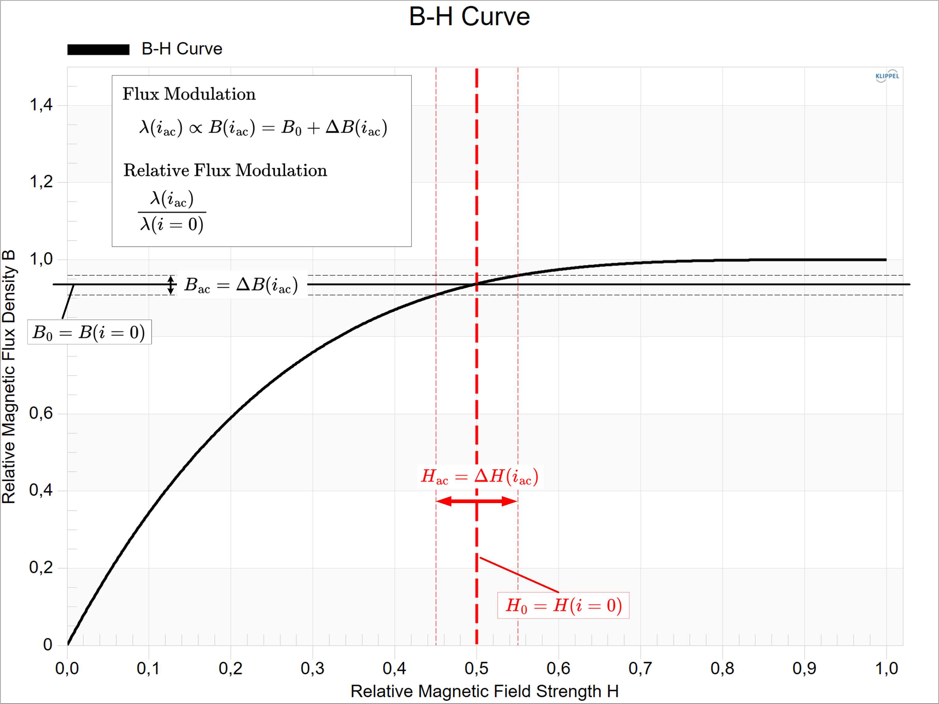
The total magnetic flux “seen” by the voice coil at its rest position \(x=0\) consists of two components:
a DC component\(\lambda_\mathrm{0}\), produced by the permanent magnet
the flux linkage\(\lambda(i_\mathrm{ac})\), produced by the electric AC current in the voice coil.
If the AC voice-coil current significantly alters the total magnetic flux and the permeability of the iron in the skin region,
the effective permeability, and therefore the inductance, becomes modulated.
However, if the iron is already highly saturated by the static flux from the permanent magnet, this variation is typically small.
In FLSI, the flux modulation is represented as the relative effective flux linkage
\[\frac{\lambda(i_\mathrm{ac})}{\lambda(i=0)},\]
measured at the voice coil’s rest position \(x=0\).
B-H curve of iron explaining flux modulation
Flux modulation primarily contributes to harmonic distortion at frequencies above the loudspeaker’s resonance frequency.
The flux modulation identified in FLSI is valid for AC signals at typical audio frequencies.
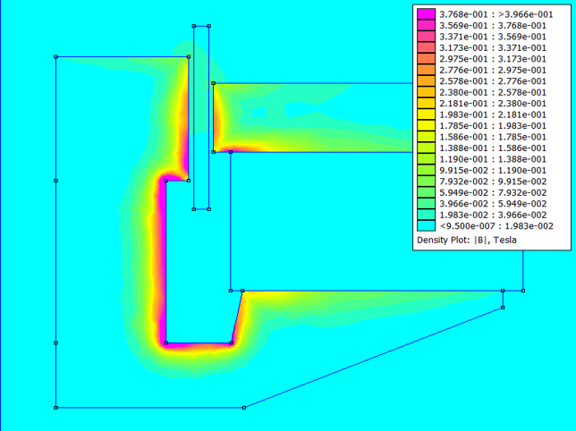
If the skin effect’s penetration depth, \(\delta_\mathrm{skin}\), is significantly smaller than the pole piece diameter,
\(d_\mathrm{pole}\) — which is typically the case already at low frequencies (20 Hz) —
the flux modulation affects only the voice coil’s self-inductance and has no significant impact on \(Bl\):
\[Bl(i) \approx \text{constant with respect to } i, \quad \text{when } \delta_{\mathrm{skin}} \ll d_{\mathrm{pole}}\]
Flux Density with 20 Hz sinusoidal excitation, visualizing the skin effect (FEMM)
Note that the effective flux modulation is not a parameter in the strict sense, as the nonlinear curve shape
depends on the particular excitation signal, its bandwidth, frequency shaping, and other signal characteristics.
The dependency of the mechanical resistance \(R_\mathrm{ms}(v)\) on the voice coil velocity \(v\) is a dominant
nonlinearity in micro-speakers and other transducers that have relatively small motor systems, including smaller woofers.
This nonlinearity can be usually neglected in larger woofers.
The nonlinear variation of \(R_\mathrm{ms}(v)\) is not caused by the mechanical motion of the diaphragm or other mechanical elements,
but instead arises from the nonlinear air-flow resistance in small structures, typically within the transducer’s motor.
This effect can be easily verified by performing a measurement in vacuum, where the nonlinearity disappears.
In FLSI, this acoustic parameter is reflected into the mechanical domain via the effective radiation surface area \(S_\mathrm{d}^2\),
so that the resulting nonlinearity becomes comparable to \(R_\mathrm{ms}(v \approx 0)\), which represents the small-signal mechanical losses.
The nonlinearity of \(R_\mathrm{ms}(v)\) leads to a significant increase in mechanical damping,
resulting in nonlinear amplitude compression of the fundamental near the resonance frequency
and the generation of substantial harmonic and intermodulation distortion.
In LSI2/LSI3 \(R_\mathrm{ms}(v)\) was modeled using a power series expansion
\[R_{\mathrm{ms}}(v) = r_1 \, v + r_2 \, v^2,\]
which usually leads to a parabolic curve shape when the asymmetry of \(R_\mathrm{ms}(v)\) is small.
In FLSI, the shape of the nonlinearity was refined to more accurately represent nonlinear flow resistance.
Since the nonlinear (large-signal) drag force \(F_\mathrm{D}\), caused by flow resistance, is proportional
to the square of the mean air particle velocity,
the nonlinear parameter \(R_\mathrm{ms}(v)\) can therefore be modeled as a linear function of velocity,
with different behavior between inflow and outflow:
\[\begin{split}R_{\mathrm{ms}}(v) =
\begin{cases}
r_+ \, v & \text{for } v \ge 0 \\
r_- \, v & \text{for } v < 0
\end{cases}\end{split}\]
This approximation is consistent with quadratic drag behavior in nonlinear flow regimes.
The asymmetry of the \(Bl(x)\) curve can be represented by a single value, as defined in
Nonlinear Parameters.
It can also be calculated for different voice coil offsets, \(x_\mathrm{off}\),
and amplitudes, \(x_\mathrm{ac}\), resulting in \(a_{\mathrm{Bl}} \left(x_\mathrm{ac}, x_\mathrm{off} \right)\).
An asymmetry is considered negligible if \(a_{\mathrm{Bl}} \left(x_\mathrm{ac}, x_\mathrm{off} \right) < 5\%\).
A so-called \(Bl(x)\) symmetry region is displayed as a gray area in the \(Bl(x)\) symmetry window,
plotted against \(x_\mathrm{off}\) and \(x_\mathrm{ac}\).
The \(K_\mathrm{ms}(x)\) or \(K_\mathrm{mt}(x)\) (in case of closed box speaker type)
symmetry range represents the region where the stiffness variation remains below 5%, as
function of displacement amplitude (x-axis) and voice coil offset (y-axis).
It is calculated in a similar way as the \(Bl(x)\) symmetry range.
Within the desired operating range, the rest position — indicated by the thick black
curve — should lie entirely within the symmetry range (gray area).
In this case, \(K_\mathrm{ms}(x)\) (or \(K_\mathrm{mt}(x)\)) asymmetries can be considered negligible.
A typical indicator of a geometrical asymmetry in the spider (e.g., cup shape) or surround (e.g., half-wave profile) is
when the symmetry region runs parallel to the x-axis but never intersects it.
In some cases, improved alignment of the suspension components may help.
However, the root causes of asymmetry typically need to be identified by separating the spider and surround and using finite element analysis (FEA).
The symmetry range, displayed as gray area, was was changed from 5% in LSI to 20% in FLSI.
We have learned that a symmetry range limited at 5% was too critical, leading to an overestimation
of the negative effects.
The red lines in the \(Bl(x)\) and \(K_\mathrm{m}(x)\) symmetry range charts
represent their symmetry points.
Ideally, the symmetry points coincide with the x-axis.
The symmetry point in the nonlinear \(Bl(x)\) curve is where a negative and positive displacement x
will produce the same force factor
FLSI calculates parameter-based displacement limits according to standard IEC 62458 or based on manual thresholds.
Force Factor:
The maximum displacement \(x_{\mathrm{Bl}}\) is limited by excessive nonlinear \(Bl(x)\) distortion.
It is defined as the smallest displacement for which the relative force factor
\[\frac{Bl(x)}{Bl(0)}\]
reaches a defined threshold \(Bl_{\mathrm{min}}\) (default: 82%):
The maximum displacement \(x_{\mathrm{C}}\) is limited by excessive nonlinear stiffness/compliance distortion.
It is defined as the smallest displacement for which the relative mechanical compliance (which is the reciprocal of stiffness)
For free air systems, \(K_\mathrm{m}\) corresponds to \(K_\mathrm{ms}\). For speaker systems comprising a
closed back chamber, \(K_\mathrm{m} \equiv K_\mathrm{mt}\) (total stiffness comprising the
mechanical suspension \(K_\mathrm{ms}\) and the air spring stiffness \(K_\mathrm{mb}\)).
Inductance:
The amplitude modulation caused by the nonlinear self-inductance is directly related to the variation
of the magnitude of the blocked electrical impedance with displacement \(x\).
This impedance, comprising only the DC resistance and the voice coil (not considering back-EMF), is defined as:
\[Z_{\mathrm{e}}(f,x) = R_{\mathrm{e}} + Z_{\mathrm{L}}(f,x, i \approx 0)\]
The displacement limit \(x_{\mathrm{L}}\) is defined as the smallest displacement for which
the relative impedance magnitude
\(f_{2}\) is the frequency of the modulated voice tone and set to \(f_{2} = 8.5 f_{\mathrm{res}}\).
For free air and vented box measurements, \(f_{\mathrm{res}}\) corresponds to the transducer’s resonance frequency \(f_{\mathrm{s}}\).
In other complete system measurements (i.e., closed box), \(f_{\mathrm{res}} = f_{\mathrm{c}}\).
Note
\(x_{\mathrm{L}}\) can be read from the inductance nonlinearity chart Lossy Inductance (x):
It corresponds with the minimum displacement, where the inductance impedance magnitude curve at \(f_{2}\),
plus the small signal DC resistance \(R_\mathrm{e}\),
(highlighted by a thick curve) varies by \(\pm Z_{\mathrm{max}}\).
Doppler:
The maximum displacement \(x_\mathrm{D}\) is defined as the point where the Doppler Effect introduces excessive phase modulation.
It can be estimated analytically using the expression
\(Bl(x)\) may reach its maximum at a displacement other than the rest position \(x=0\) if the curve is asymmetric.
\(Bl_\mathrm{max}\) denotes the maximum \(Bl\) value over the entire modeled displacement range.
This value may slightly differ from the maximum displacement measured by the laser due to small modeling and measurement inaccuracies.
The complete modeled and measured displacement signals can be compared in the
Displacement Waveform Chart.
Maximum Port Velocity:
The maximum of the modeled mean spatial particle velocity \(v_{\mathrm{p,modeled}}\) in the port
can be calculated based on the full nonlinear lumped parameter model and precise values of
the effective radiation area of the transducer and port, specified on the FLSI’s property page.
Bl(x) Symmetry point x sym,bl:
This parameter is a single-value representation of the symmetry point curve displayed in the
Bl(x) Symmetry Range window
at the displacement \(x_\mathrm{prot}\).
The symmetry point is specified in the standard IEC 62458.
Km(x) Symmetry point x sym,k:
This parameter is a single-value representation of the symmetry point curve displayed in the
Km(x) Symmetry Range window at the displacement \(x_\mathrm{prot}\).
It is calculated in a similar way as the \(Bl(x)\) symmetry point.
Bl(x) Asymmetry:
The \(Bl(x)\) asymmetry can be assessed by a single value, as defined in
Nonlinear Parameters.
using the stiffness at the negative and positive maximum displacement ± \(x_\mathrm{prot}\) of the measured \(K_\mathrm{m}(x)\)-curve.
The sign of \(a_\mathrm{k}\) corresponds to the direction of the DC displacement generated dynamically by the
nonlinear rectification process of the displacement.
It has the same sign like the stiffness symmetry point.
The stiffness asymmetry parameter is specified in the standard IEC 60268-22.
Port Asymmetry:
This value is displayed only for vented box systems.
The asymmetry of the nonlinear port resistance \(R_\mathrm{ap}(v_\mathrm{p})\)
(see the lumped parameter model of the ported system in section Speaker System Modeling)
can be assessed using the following equation:
This calculates the asymmetry in the nonlinear port resistance at the maximum peak velocities observed during the measurement.
At the negative peak velocity \(-v_{\mathrm{p,peak}}\), air is sucked into the enclosure.
At the positive peak velocity \(+v_{\mathrm{p,peak}}\), air is pushed out of the enclosure into the ambience.
Any asymmetry of the port resistance creates a static pressure difference between the
atmospheric static pressure outside the loudspeaker enclosure and its inside.
This static pressure difference creates a DC displacement of the voice coil that has to be considered in the
system design to ensure stability and robustness.
A negative sign of \(a_\mathrm{r,port}\) means that the resistance to push air outside the enclosure
into the ambience is lower than to suck air inside, and vice versa.
Hence, the sign of the voice coil DC displacement caused by the port asymmetry corresponds with the sign of the asymmetry value.
is a single value representation of the nonlinear force factor \(Bl(x)\), neglecting its complicated curve shape.
It plays a crucial role in determining \(x_\mathrm{prot}\) and in providing mechanical
protection for the driver during the measurement.
is a single value representation of the nonlinear compliance, neglecting its complicated curve shape.
It plays a crucial role in determining \(x_\mathrm{prot}\) and in providing mechanical
protection for the driver during the measurement.
The following sections explain the metrics used to evaluate the accuracy of the identified nonlinear parameter model
in both the small and large signal domains.
Error values below 5% are typically considered good.
If any error metrics exceed predefined thresholds, the FLSI will display warning or error messages.
The error between the fitted voice coil displacement and the laser-measured displacement of the small signal measurement
(LINEAR MODE) is expressed as the normalized root mean squared error (NRMSE)
\(H_\mathrm{x}(f_n)\) is evaluated solely at low frequencies, typically below approximately four times the DUT’s resonance frequencies,
because the laser signal becomes noisy at higher frequencies.
This error metric is highly valuable to evaluate the accuracy of the identified\(Bl(x=0)\), under the assumption that
the laser is correctly calibrated,
the optical conditions are good, and
no severe rocking modes occur.
Note that if an inaccurate \(Bl(x=0)\) is imported on the property page, this error will increase.
The error between the fitted voice coil displacement and the laser-measured displacement of the large signal measurement
(NONLINEAR MODE) is expressed as the NRMSE
The voltage and current waveforms show the electrical signals measured by the KA3’s sensors, while the sound pressure waveform represents the microphone signal.
All signals are displayed in the time domain.
The spectra show how the signals are distributed across frequencies in the frequency domain.
The following curves are available:
Fundamental
The multi-tone stimulus used by the FLSI consists of many different frequencies.
This curve displays the measured signal at those frequencies.
You can right-click in the chart and press Mark Data Points, or use the A key to highlight them.
Note that a single low-frequency tone is applied to measure the voice coil’s DC resistance.
Noise
A short noise floor measurement is performed at the start of the LINEAR MODE.
Note that the noise floor measurement in the LINEAR MODE is shorter than in the NONLINEAR MODE.
As a result, the noise floor spectrum has a lower frequency resolution than the Distortion+Noise curve.
Distortion+Noise
In an ideal, linear, noise-free system, no signal energy exists between the fundamental frequencies.
However, a loudspeaker is a nonlinear system that generates new frequency components as combinations of the fundamental frequencies.
The laser-measured displacement is displayed as both a waveform and a spectrum.
In addition to the measured signal, the displacement calculated from the nonlinear lumped loudspeaker model is displayed.
The deviation between the modeled and measured displacement is typically very low.
However, if an inaccurate \(Bl(x=0)\) is imported through the property page,
the deviation will be significant because the mechanical calibration will be incorrect.
You can right-click in the chart and select Show all Curves to display the displacement
calculated using a linear lumped parameter model.
In a highly nonlinear loudspeaker, the deviation between the peak displacement of the nonlinear and linear models can exceed 50%.
Comparing the two modeled displacement signals indicates the error introduced by linear simulations,
such as those used in linear speaker protection systems.
The sound pressure output for the multi-tone signal used in the NONLINEAR MODE can be estimated through the identified nonlinear model.
This numerical simulation also allows for the evaluation of the nonlinear distortion generated by any nonlinearity present
in the model, providing valuable insights into how each nonlinearity contributes to the overall distortion.
This capability is highly useful for identifying the root cause of the dominant nonlinear distortion.
It can guide efforts to optimize the relevant components of the loudspeaker assembly.
Furthermore, it highlights which nonlinearities have a negligible impact on the speaker’s performance.
For example, distortion components below approx. 1% are typically considered minor and generally don’t require significant attention.
Additionally, the simulation can evaluate the impact of various factors — such as stimulus level, linear transducer parameters,
and enclosure type (e.g., closed, vented, or passive radiator) — on the total distortion.
The FLSI displays the distortion components in two ways:
SPL Spectrum with Distortion Components: This window displays the spectrum for each individual distortion component,
offering insights into the distortion characteristics of each nonlinearity.
It shows, for example, in which frequency range a nonlinearity is most dominant.
These distortions arise from the various combinations of fundamental frequencies.
The distortion components include both harmonic and intermodulation distortion.
Relative Nonlinear Distortion Components: These single values displayed in a table in the Large Signal Parameters window
show the overall distortion resulting from all the nonlinearities.
The relative distortion components are calculated using the ratio between the RMS value of each
distortion component, denoted as \(p_{\mathrm{RMS},i}\), and the total sound pressure \(p_{\mathrm{RMS,total}}\):
\[p_\textrm{RMS} = \sqrt{\frac{1}{T}\int_{t=0}^T p\left( t \right)^2 \mathrm{d}t}\]
where T is the duration of the multi-tone measurement block used in the nonlinear parameter fitting.
The following nonlinear distortion components are calculated:
Dtotal / Total Distortion (modeled)
Total modeled relative multi-tone distortion.
Dbl / Force Factor
Relative distortion contribution of the nonlinear force factor \(Bl(x)\).
Dk / Stiffness
Relative distortion contribution of the nonlinear mechanical stiffness \(K_\mathrm{m}(x)\).
Dr,int / Internal Mechanical Damping
Relative distortion contribution by the nonlinear internal damping of the suspension materials.
This is also called material damping.
It includes nonlinear mechanical creep, mechanical hysteresis and nonlinear viscous damping.
Dr,ext / External Resistance Rms(v)
Relative distortion contribution of the nonlinear external damping \(R_\mathrm{ms}(v)\).
This depends on the voice coil velocity \(v\) and is caused by the air flow resistance near
the magnetic gap and in the transducer’s motor.
It mainly (but not only) occurs in small transducers such as micro-speakers.
Dlx / Inductance (x)
Relative distortion contribution of the nonlinear displacement-dependent inductance \(Z_\mathrm{L}(x,f)\).
Dλi / Flux Modulation
Relative distortion contribution of the nonlinear flux modulation \(\lambda(i)\).
Dreluct / Reluctance Force
Relative distortion contribution caused by the reluctance force.
Dsd / Radiation Area Sd(x)
Relative distortion contribution of the nonlinear radiation area \(S_\mathrm{d}(x)\).
The identification of this distortion component requires a microphone.
Note
The relative total distortion value Dtotal is smaller than the arithmetic sum of all distortion components.
This is because the distortion components are relative RMS values.
If all distortion signals are orthogonal, the total distortion would equal
the square root of the sum of the squares of all distortion components.
\[D_\textrm{total,abs} = \sqrt{\sum_i^N D_i^2}\]
However, the distortion components are never orthogonal.
They can cancel each other in certain frequency ranges, depending on their phase relationships.
Hence, the resulting Dtotal,abs value is
always larger than Dtotal, which considers the component’s phases.
This shows the DC force caused by the asymmetric part of the nonlinear stiffness.
Fdc,bl
This shows the DC force caused by the nonlinear force factor.
Fdc,reluct
This shows the DC force caused by the reluctance force.
Fdc,rp
This shows the DC force caused by asymmetric nonlinear port behavior.
Note
Stiffness and port asymmetries generate DC forces that act in the same direction over the full frequency range where the corresponding nonlinearities are active.
In contrast, DC forces caused by the reluctance force and, in particular, the force factor \(Bl(x)\) are frequency-dependent.
For example, if \(Bl(x)\) produces a positive DC force below the resonance frequency, it will typically produce a negative DC force above resonance.
As a result, the multi-tone stimulus used in FLSI effectively excites DC forces related to stiffness, port nonlinearities, and also reluctance force
(that usually causes DC forces in a relatively narrow band).
However, DC forces caused by \(Bl(x)\)tend to partially cancel out under wideband excitation, since contributions
from different frequency ranges act in opposite directions.
Therefore, these effects may appear less critical in FLSI measurements, even though they can be significant under narrowband or single-tone excitation.
Hence, FLSI provides valuable insight into DC forces caused by most nonlinear mechanisms under realistic broadband conditions.
However, to fully assess worst-case DC displacement — particularly those driven by \(Bl(x)\) —
it is strongly recommended to perform additional measurements using sinusoidal excitation usingDIS – Distortion.
Make sure that that the laser is well adjusted and its beam is perpendicular to a bright, reflective measurement spot.
It is recommended to create a white reflective coating on the membrane so that the laser has good
measurement conditions.
If this is not possible, you can deactivate the X target protection limit and
specify a safe voltage manually.
In this case, the error is displayed as a warning and the measurement is continued even if
spikes or clipping is detected in the laser signal.
Make sure that the DUT is fixed tightly and cannot move during the measurement.
Check that the correct speaker system type is selected on the property page#
Cause:
The impedance that was recorded in the small signal measurement during the LINEAR MODE
is checked for feasibility.
The measured impedance magnitude of a speaker that is expected to have only a single
mechanical resonator (e.g., free air or closed box systems) should exhibit only a single resonance peak.
This warning is displayed if the measured impedance magnitude exhibits more than one significant resonance peak,
which indicates that the wrong speaker system type is selected on the property page.
However, additional resonances can exist. For instance, mechanical modes on the DUT’s
membrane might cause additional resonances in the electrical impedance.
Remedies:
Select the correct speaker system type on the property page, if the wrong ones is selected currently.
Note
If you are sure that you have selected the correct speaker system type, please disregard this message,
as it is not always possible to identify the speaker type automatically.
This error occurs if the linear lumped parameters cannot be identified due to unspecified reasons.
Possible reasons include (also see Supported Test Objects):
Wrong speaker system type selected on the property page.
Speaker system type is not supported (such as 6th or higher order band-pass systems or shakers mounted on a thin, free-swinging board causing multiple peaks in the electrical impedance magnitude).
Multiple speakers are connected to the amplifier in series or in parallel. This is not supported.
Electrical components (such as passive crossover) are connected to the transducer terminals.
Remedies:
Make sure that the electrical impedance looks feasible and similar to the examples below. The impedance curves must not be significantly distorted and the magnitude must not comprise more than two distinct peaks.
Make sure that the transducer is fixed tightly. It must not move around during the measurement.
Try to reduce the excitation level, in case the transducer already behaves highly nonlinear (i.e., \(Bl(x)\) drops below 25% or \(K_\mathrm{ms}\) increases by factor 8 nor more).
Contact KLIPPEL support if you cannot solve the issue based on the information given above.
High Fitting Error (LINEAR MODE / NONLINEAR MODE)#
This warning appears if the linear or nonlinear fitting error exceeded a certain threshold.
Make sure that
the correct speaker system type (closed box, vented, …) is selected
the DUT can be described by a second or 4th order mechanical system (maximum of two distinct resonance peaks in the electrical impedance magnitude)
the DUT’s resonance frequency and DC resistance is supported by the FLSI (see the specification document)
Please contact the Klippel support in case if the above statements are fulfilled.
This warning appears after the LINEAR MODE, if the target signal-to-noise+distortion ratio in the electrical signals could not be reached.
This may for example happen when measuring transducers which have very low suspension stiffness.
Usually the small-signal parameters are accurate even if this warning appears, however observe the fitting error and LINEAR MODE’s peak displacement carefully.
Also make sure that the environment is quiet during the measurement to avoid the transducer acting as a microphone, creating undesired distortion in the back-EMF.
I have installed a KCS-ID license but do not find the KCS category on FLSI’s property page#
It is required to trigger FLSI module’s license check by changing a parameter on the property page.
I.e., temporarily change the entry of the Geometry drop-down list.
Why do I get different results with the FLSI compared to the LSI3 or LPM?#
The speaker model was improved and comprises new linear and nonlinear parameters, including the nonlinear mechanical creep and the frequency-dependent inductance nonlinearity.
This enhances the accuracy of the existing linear parameters, such as resonance frequencies and Q-factors,
as well as nonlinear parameters, such as \(Bl(x)\) and nonlinear inductance.
The nonlinear inductance model was improved and extended.
The LSI2 and LSI3 algorithms identify a single nonlinear inductance curve \(L_\mathrm{e}(x)\),
assumed to be valid across the full excited bandwidth.
As a result, the identified inductance represented an average over the entire excited frequency range.
However, this simplification becomes inaccurate when shorting material is present in the transducer motor
and/or when the transducer operates over a wide frequency bandwidth.
To address this, the FLSI extends the nonlinear inductance model by a frequency-dependent nonlinearity.
The nonlinear inductance is represented by a nonlinear impedance magnitude.
FLSI employs a more insightful representation of the nonlinear self-inductance.
Whereas LSI2 and LSI3 display the nonlinearity of a pure inductance \(L_\mathrm{e}(x)\),
FLSI calculates the impedance magnitude of the inductance \(|\underline{Z}_\mathrm{L}(f,x)|\),
which is directly related to distortion behavior.
The advantages of this representation are discussed in greater detail in section Lossy Inductance (x) (see Note section).
This prevents noise in the laser signal from degrading the accuracy of the :math:Bl(x=0) estimate.
In addition, the moving mass is assumed to be constant under both small- and large-signal conditions.
As a result, \(Bl(x=0)\) may differ slightly between the small- and large-signal domains.
Such deviations can be caused, for example, by:
a shift of the voice coil rest position during large-signal operation, or
temperature-dependent changes of the permanent magnet’s field strength
What makes FLSI linear parameters more accurate than LPM parameters?#
FLSI employs a curve-fitting algorithm that is similar to LPM.
However, the fitting algorithm was significantly improved in FLSI to improve accuracy:
FLSI uses a more complex inductance model, improving fitting accuracy of the electrical impedance over the full measurement bandwidth.
FLSI identifies creep and/or leakage effects (in closed-box configurations) directly in the electrical impedance fitting, whereas LPM uses laser data — this improves fitting accuracy of the electrical impedance and parameter accuracy.
FLSI determines stimulus bandwidth, level, and averaging parameters automatically — in contrast, LPM requires manual configuration. Manual setup is more error-prone, as software feedback may not cover all cases of suboptimal settings.
FLSI identifies the moving mass (see Mechanical and Acoustical Calibration) in the large signal measurement, preventing noise in the laser signal from degrading the accuracy of the \(Bl(x=0)\) estimate.
FLSI’s server-based licensing infrastructure enables customers to
continuously benefit from the latest measurement technology, models, and software improvements.
The FLSI module installed on the PC communicates with the KA3 and acquires the measurement signals.
The actual parameter identification is performed on an FLSI server, which returns the identified parameters to your PC.
See Privacy Policy for information about the data exchanged with the server.
FLSI uses the command-line tool curl to communicate with the FLSI servers.
If any software restriction policy is in place on your PC, make sure that you are permitted to execute curl and
that it is allowed to establish HTTPS connections to the FLSI servers.
dB-Lab installs curl under the path
%ProgramData%\Klippel\<DB-LABNAME>\Scripts5\Klippel\Library\curl\CURL.EXE.
%ProgramData% usually links to C:\ProgramData and <DB-LABNAME> is usually RnD,
if only a single dB-Lab is installed on your computer.
FLSI servers are accessible through the domain *.klippel.services (i.e., nix.klippel.services).
All communication is encrypted using TLS 1.2 or higher, with TLS 1.3 preferred, over the standard HTTPS port (443).
If a firewall is in place, make sure it allows outgoing HTTPS connections (port 443) to *.klippel.services.
If your network traffic is routed through a proxy server, curl must be configured accordingly because it does not automatically use the Windows proxy settings.
Open your preferred file manager and go to folder %ProgramData%\Klippel\RnD\Scripts5\Klippel\Library\curl\ (if your dB-Lab installation is not called RnD, then modify the URL according to the name of your dB-Lab’s installation)
Create a file in this folder with the name .curlrc (no file ending) and open it in a text editor
Add the following line to the file, replacing <IP_ADDRESS> and <PORT_NUMBER> with your proxy server settings: proxy=<IP_ADDRESS>:<PORT_NUMBER> (e.g. proxy=192.168.10.10:8080 )
Verify that the FLSI server domain can be reached by
opening the URL https://nix.klippel.services in your browser
Expected Result
An HTTP 4xx status code (for example, 401 or 403) is expected to be displayed in the browser.
If the browser shows an error like Can’t open the page because the server can’t be found or similar, a firewall may be blocking access to the Klippel servers.
Remedy:
Configure the firewall to allow outgoing HTTPS connections to all subdomains of klippel.services, as the server names may change over time.
A software restriction policy may be in place in your company preventing executable (.exe) files from being run.
To test if you have the permission to run the required software curl,
open a Windows Command Prompt (press the Windows button and type cmd).
Run %ProgramData%\Klippel\RnD\Scripts5\Klippel\Library\curl\CURL.EXE"https://nix.klippel.services"
(if your dB-Lab installation is not called RnD, substitute RnD with the name of the dB-Lab installation name that you are using).
Expected Result
An HTTP 4xx status code (such as 401 or 403) should be displayed.
If curl reports Could not resolve host, the DNS, proxy, or firewall configuration is likely incorrect.
If it reports a Windows error code (such as 1260), curl is likely to be blocked by a software restriction policy.
Remedy:
%ProgramData%\Klippel\RnD\Scripts5\Klippel\Library\curl\CURL.EXE must be permitted to execute.
You may have to contact your IT department who can grant the required permissions.
If a proxy server is used in your network infrastructure, curl must be configured accordingly (see above).
This Privacy Policy applies to the server-based components of the measurement software provided by Klippel GmbH.
The software is intended for professional and technical use by organizations worldwide.
Technical Data is stored independently from Connection Data and Statistical Data.
It is stored in anonymized form and cannot be mapped to individual users or organizations.
This Privacy Policy may be updated to reflect technical, legal, or regulatory changes.
The current version will always be made available through the software documentation.
Gerbet, L.C. Zhu, W. Klippel, “Validating Nonlinear Transducer Motor Simulations with Measurements”, ISEAT Convention 2025
Klippel, “Nonlinear Large-Signal Behavior of Electrodynamic Loudspeakers at Low Frequencies,” J. Audio Eng. Soc., vol. 40, pp. 483-496 (1992).
Klippel, “Dynamic Measurement and Interpretation of the Nonlinear Parameters of Electrodynamic Loudspeakers,” J. Audio Eng. Soc., vol. 38, pp. 944 - 955 (1990).
Klippel, “Nonlinear Modeling of the Heat Transfer in Loudspeakers,” presented at the 114th Convention of the Audio Eng. Soc., 2003 March 22–25, Amsterdam, The Netherlands, Preprint.

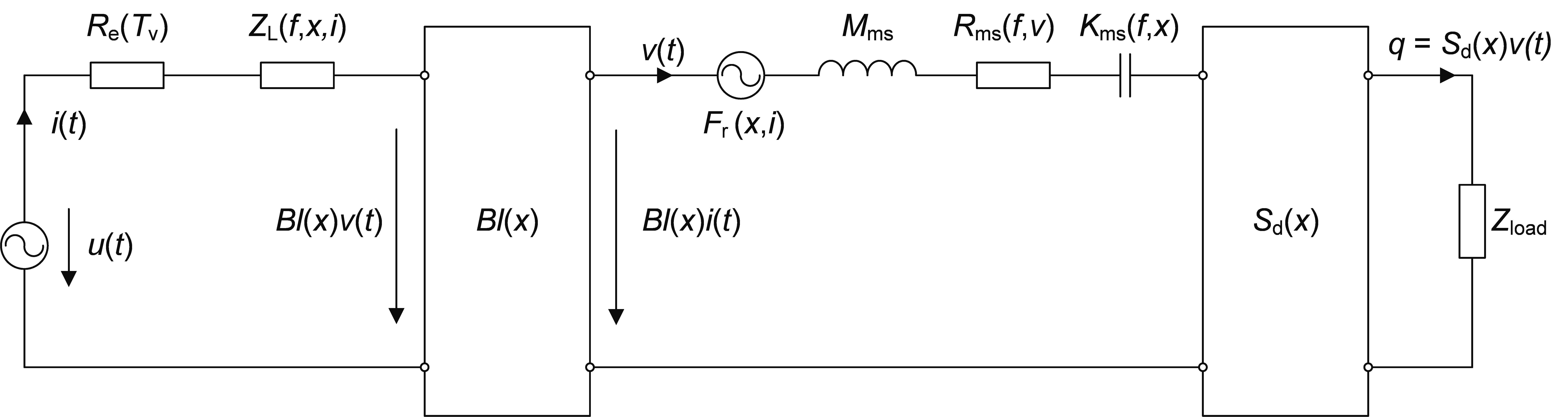
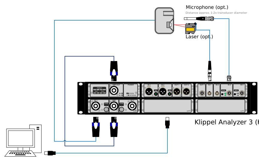
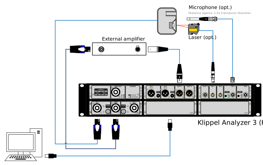
 to setup the
routing. Set the correct output channel (AMP card or XLR Card if an external
amplifier is used) and input channels for the optional external sensors.
to setup the
routing. Set the correct output channel (AMP card or XLR Card if an external
amplifier is used) and input channels for the optional external sensors.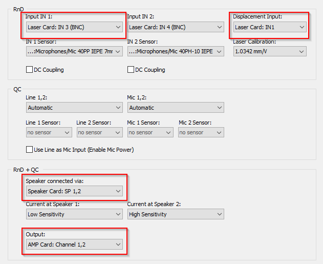
 Select Database in the dB-Lab software. Create
  a new
FLSI Fast Large Signal Identification operation, open its Properties by right-clicking on the operation and set up the
measurement as follows. It is assumed that the hardware is set up as described in Hardware Configuration
and the laser and the microphone are connected to the KA3.
a new
FLSI Fast Large Signal Identification operation, open its Properties by right-clicking on the operation and set up the
measurement as follows. It is assumed that the hardware is set up as described in Hardware Configuration
and the laser and the microphone are connected to the KA3.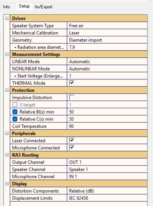
 Run button.