SCN – Scanning Vibrometer

Overview

Scanning Vibrometer Measurements

The Scanning Vibrometer (SCN) performs a non-contact measurement of the mechanical vibration and the geometry data of cones, diaphragms, panels and enclosures.

One rotational and two linear actuators (\(\phi\), \(r\), \(z\)) move a laser displacement sensor over a user-defined grid. At each measurement point the transducer is excited by a stimulus giving sufficient spectral resolution and high SNR in the measured response over the whole audio band.

The collected geometry data can be exported to other FEA/BEA applications while the vibration data can be analyzed within the SCN software.

Modern techniques of image processing are used for enhancing relevant information, suppressing noise and animating the vibration as a stroboscopic video. The sound pressure output in the far field and the directivity pattern are calculated and the contribution of each vibrating point on the vibrating surface is visualized. The software indicates critical vibration pattern and uses a decomposition technique for separating radial and circular modes.

Warning

The Scanning Vibrometer hardware contains moving parts that are automatically controlled during operation. Make sure staff is not entering the working area during operation. Pay caution when setting up the device or during any other interaction with the machine.

SCN Putting into Operation

Overview

The Klippel Scanning Vibrometer comprises the Scanner Hardware and the Klippel Scanning System software for controlling the measurement of loudspeaker vibrations and for the data analysis.

This chapter is concerned with the Software Installation and the Setup of the Scanning System. If no Hardware is available, then the Klippel Scanning System software can still be used for analyzing existing scanning data.

See also

Additional instruction and knowledge to get familiar with the system can be found at:

Online Training #2 Vibration and Radiation Behavior of Loudspeakers Membrane

Visit www.klippel.de/training for easy step-by-step instructions, basic theory and advice on how to interpret your measurement results correctly.

The training consists of a short video and a handout. At the end of the training you can check your knowledge by doing a multiple choice test.

Software Installation

The Klippel Scanning System requires an installation of the Klippel dB-Lab software, which supplies capabilities of measuring transfer functions and performing mathematical calculations.

During the installation an appropriate dB-Lab installation is selected which will be activated at each startup of the Klippel Scanning System.

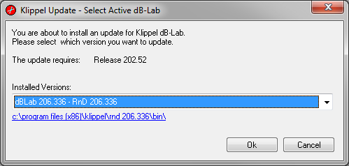
If multiple installed dB-Lab versions are found, the Klippel dB-Lab Activation dialog will appear to let you choose an appropriate installation.

Requirements

The Klippel Scanning System has no deviant requirements than the Klippel dB-Lab, which is required as basis for the installation.

• PC Operating System [1] : Microsoft Windows 7, 8 or 10 | Klippel recommends using Windows 10 or higher
• Min. CPU requirements [2] : Core 2 Duo 2.5GHz or equivalent

  recommended: Core i5 2.5GHz or equivalent

• 4GB RAM

• Min. 1 GB free disk space, plus disk space for measurement results [3]

• Internet connection strongly recommended for online-support

• PC monitor with minimum 1024x768 pixel screen resolution

  recommended: 1920 x 1080 pixel

• 2 USB 2.0 interfaces

[1]

While there are no known significant problems with Windows Vista or the respective server systems (Windows Server 2003, 2008 or 2011), they are not regularly tested and we can provide only limited support.

[2]

These specifications are sufficient for most applications running in dB-Lab. For applications that create or process significant amount of data, a high end system (i7 or equivalent, 64 bit Windows, 8GB RAM) ensures smooth, efficient and uninterrupted operation

[3]

 When planning a new PC, also consider the necessity of an automated regular backup to external storage

Please follow the instructions on the CD to install the required software components for the Klippel Scanning System.

If no Scanner Hardware is available then it is recommended to start now with the Tutorial 1 – Viewing SCN Results to get a quick introduction on how to use the Klippel Scanning System for analyzing loudspeaker vibration scans.

Otherwise please continue with the Setup of the Scanning System.

Setup of the Scanning System

This section describes the necessary steps to bring the Scanner Hardware into operation. It starts with the Mounting Instructions of the Scanner Hardware and a complete List of Parts.

Afterwards follows the Connection Setup of the Scanner Hardware and finally a step by step guide is given how to conduct a First Calibration of the Scanner.

Mounting Instructions

The Mounting Instruction is dedicated to SCN hardware revision 2.0.

For older hardware revision, some steps could differ slightly.

Older manuals are available from the KLIPPEL support.

Preparations at the Turntable

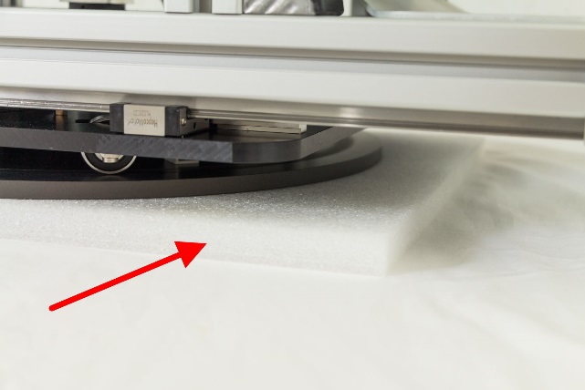
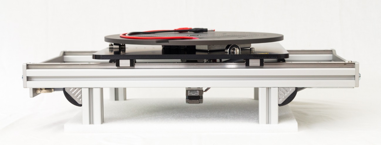
1. Unpack the Turntable and put it in upside-down position.

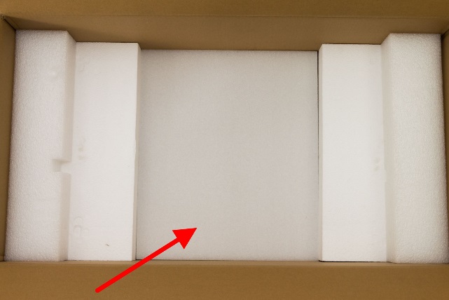
   Put it on the foam piece from the transport packaging to avoid any damages or scratches.

   

   

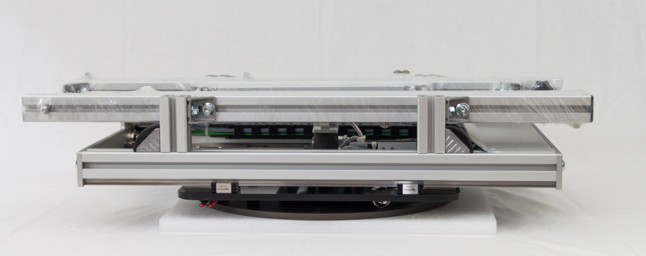
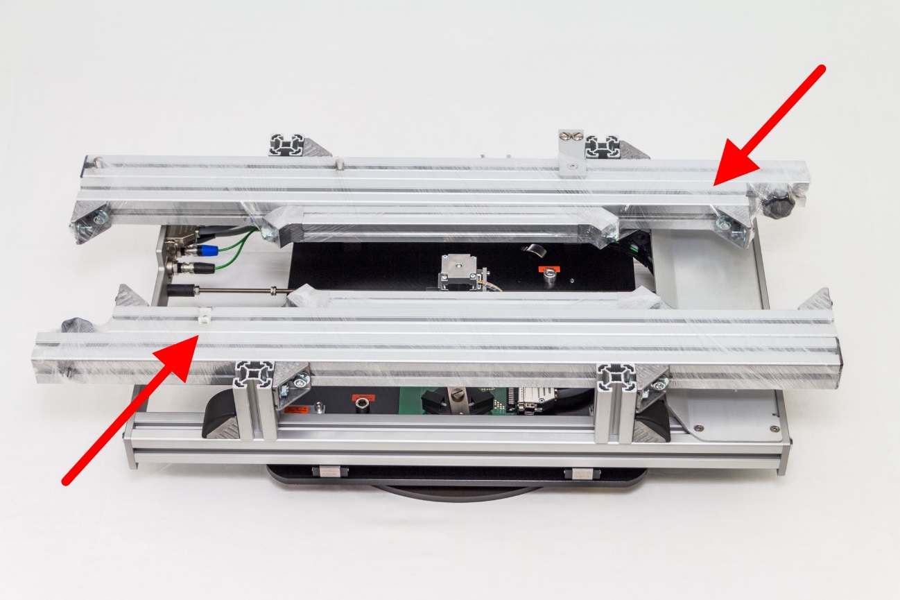
2. Remove the six wrapped bars from their shipping position.

   (13mm wrench needed)

   

   

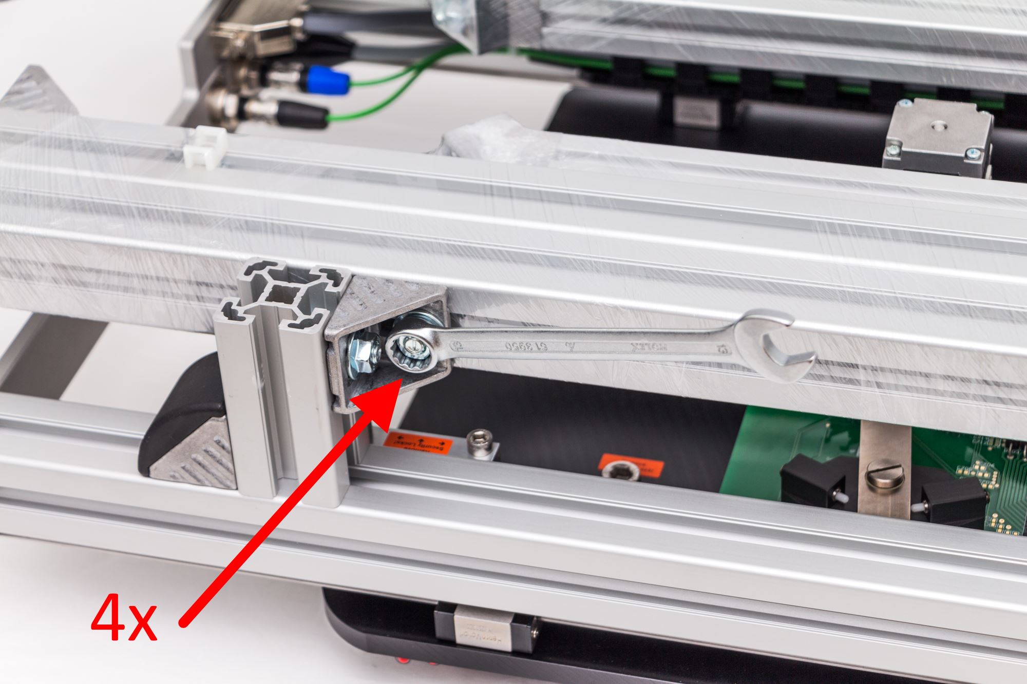
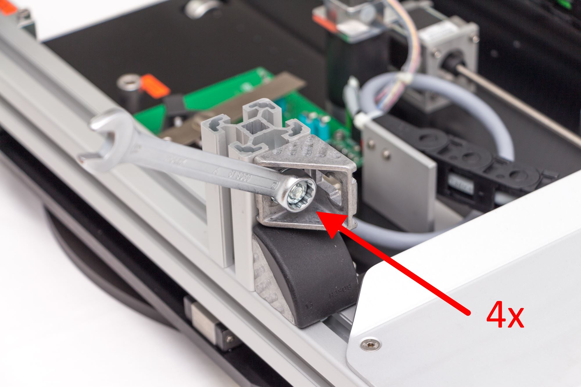
3. Remove the four angle brackets by unscrewing all eight screws.

   The angle brackets will be needed later in step 15.

   

4. Remove both R-axis shipping locks.

   (5 mm hex-wrench needed)

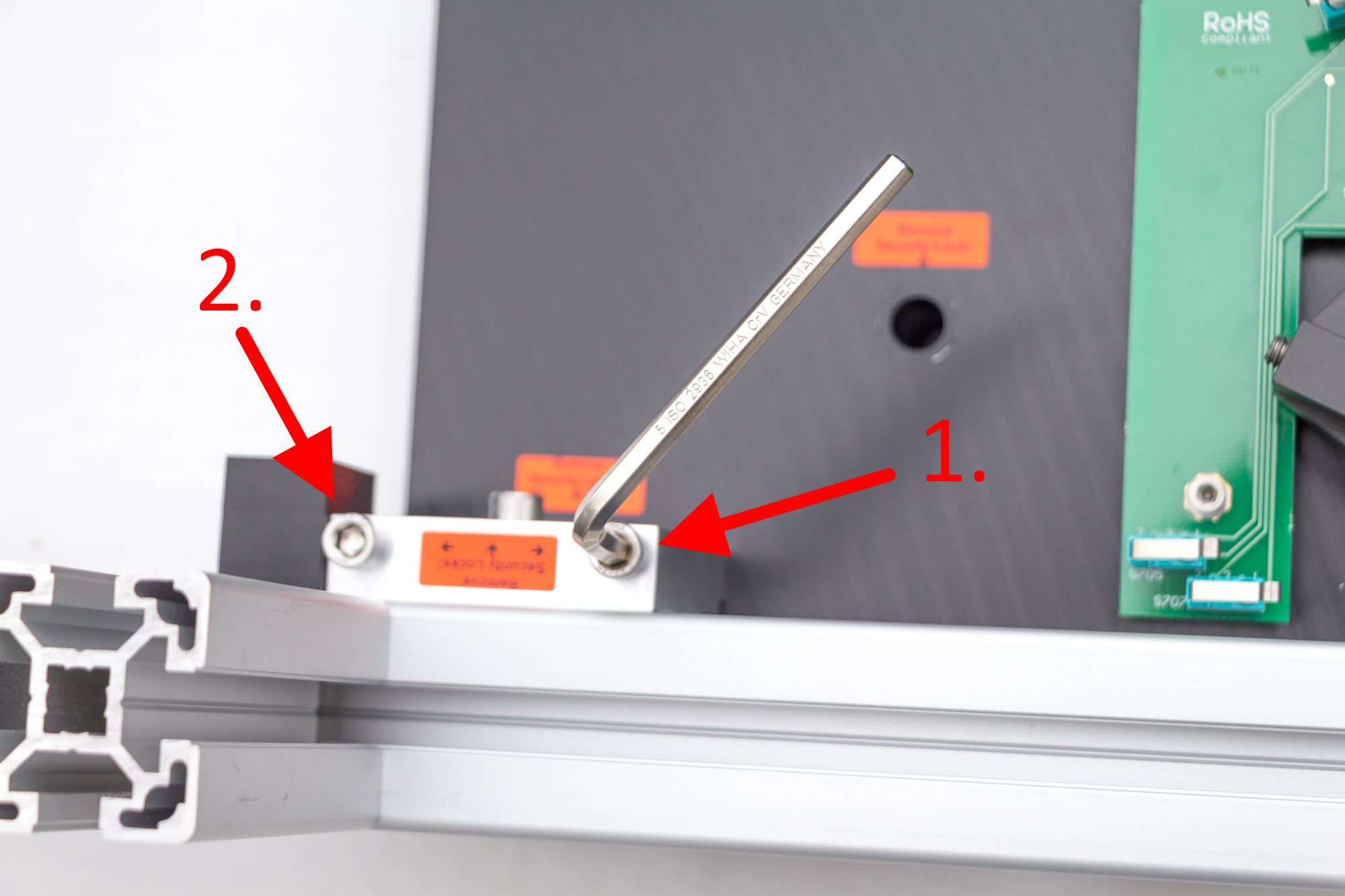
   (5 mm hex-wrench needed)

   Remove all three screws at each R-axis shipping lock before removing the lock.

   

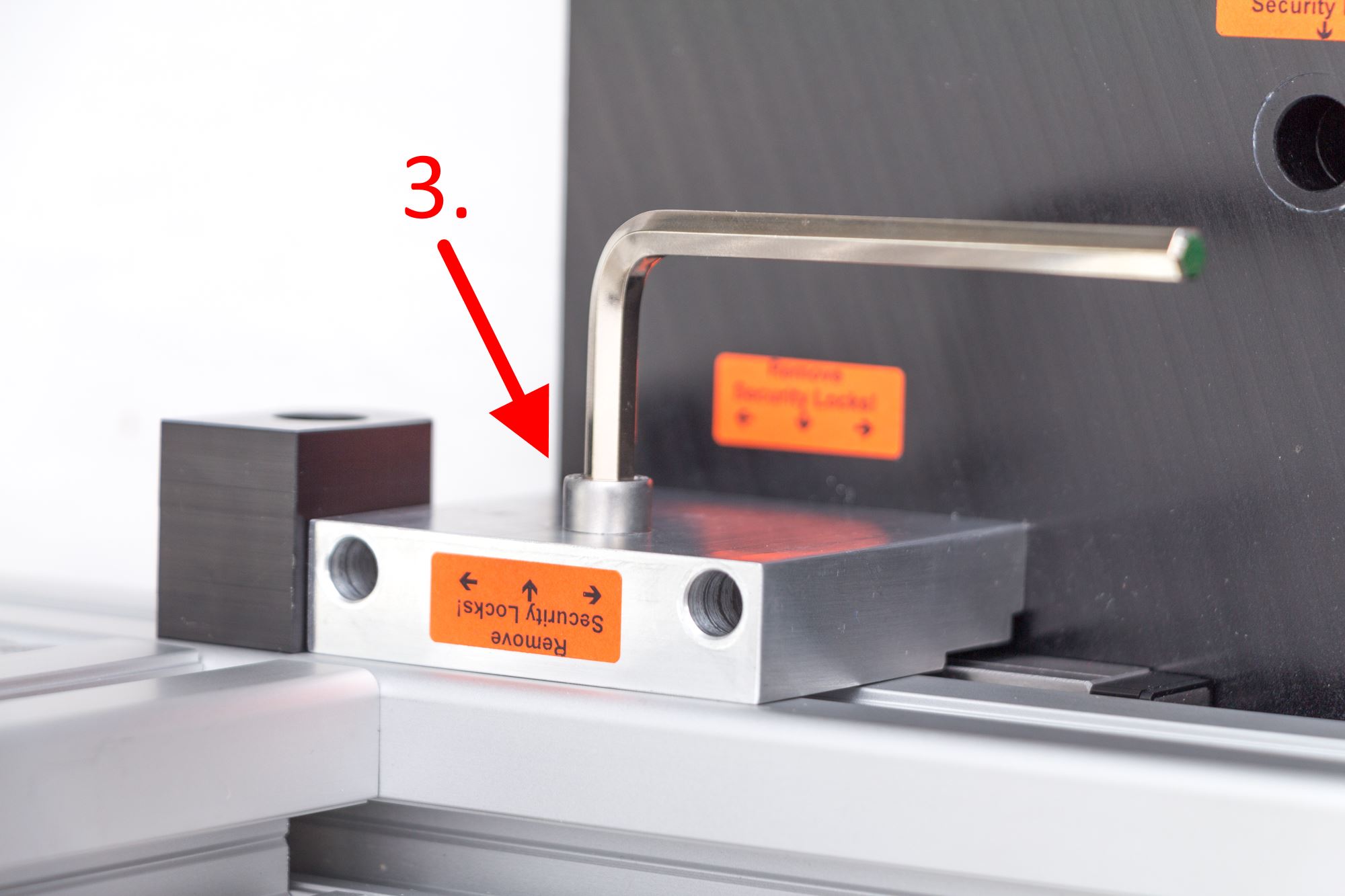
5. Remove both Phi-axis shipping locks.

   

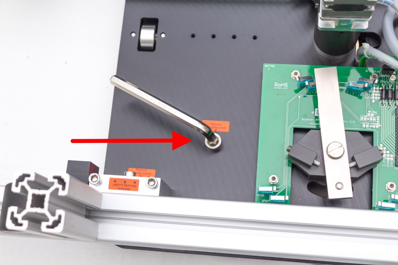
   (8mm hex-wrench needed)

6. Put the Turntable in vertical position.

   Keep the foam piece below it, to protect it from scratches.

   

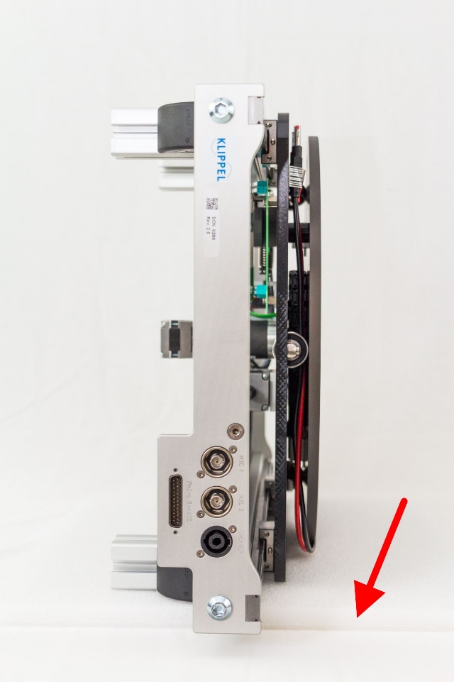
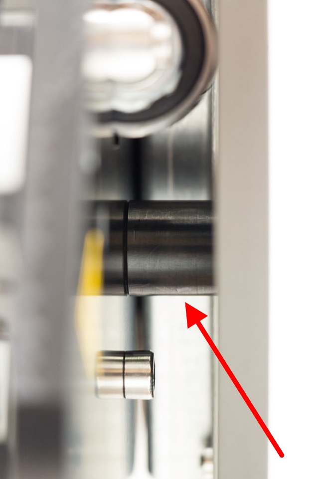
   Remove both Phi-axis shipping lock spacer, which are between the grey turntable and the black base plate. By slightly pushing the turntable plate away from the base plate they are falling out of the gap between both plates.

7. Put the Turntable in normal horizontal position.

   

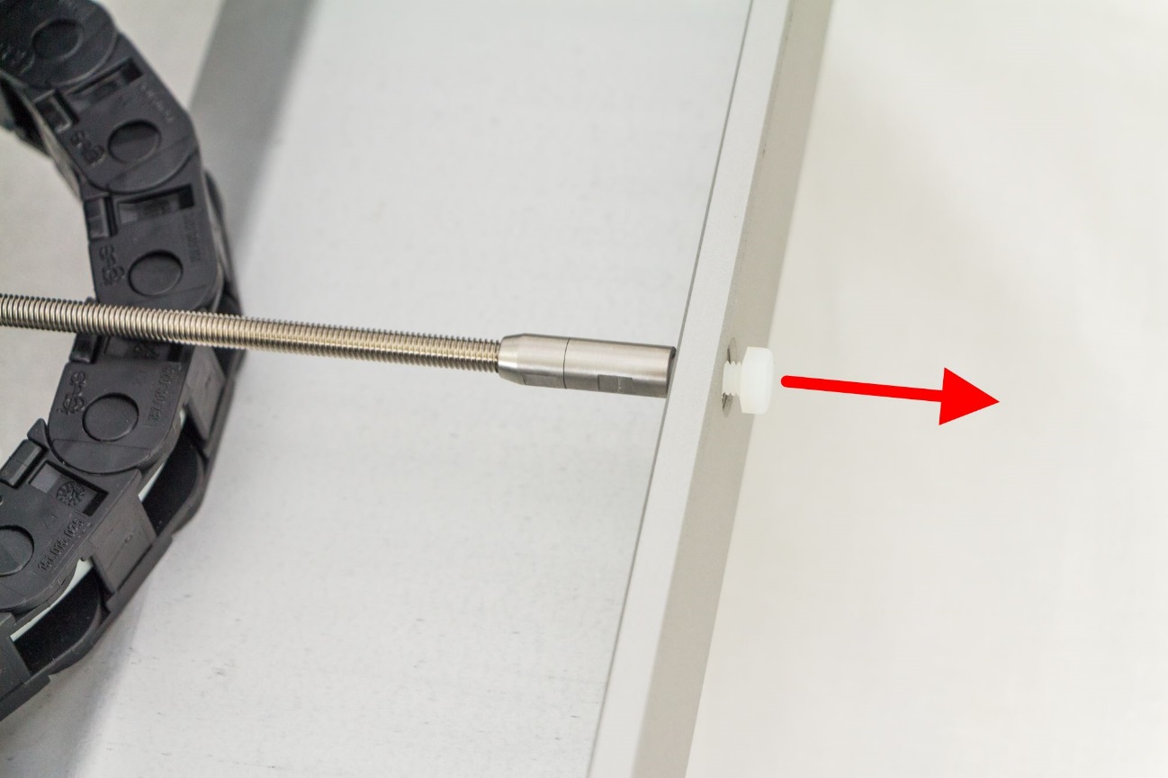
8. Fix the R-axis:

   Remove the M6 plastic shipping lock screw.

   

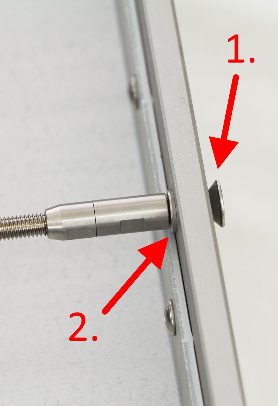
   Insert M6 x 12 mm countersunk hex screw and washer.

   They can be found in the plastic bag labeled “spare parts”.

   

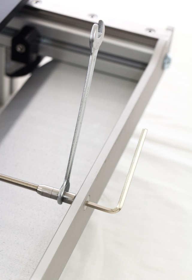
   Fix the R-axis spindle by holding the spindle and nut in its default position and fixing the screw. (8 mm wrench and 4 mm hex-wrench needed)

Mounting the Z-axis to the bottom frame:

9. Unwrap the six bars which were removed from its shipping position mounted at the Turntable (step 2).

10. Putting them on the transportation packaging foam pieces for an easier assemble.

    

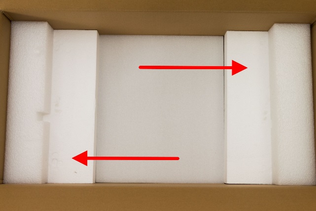
11. Place the two horizontal and vertical bars as shown in the picture.

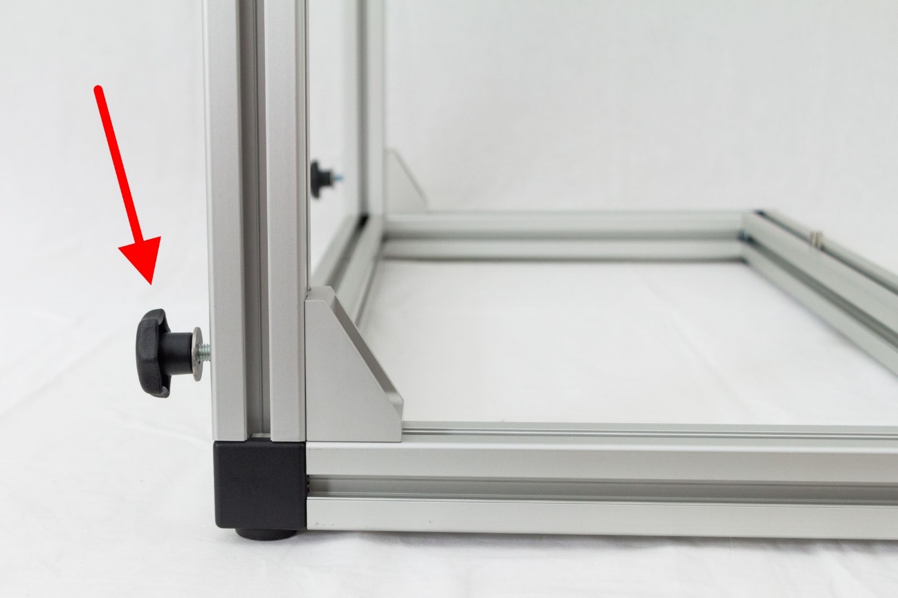
1. The vertical bars have a black plastic hand screw at the bottom end.

   It must be directed to the ground.

2. At the upper end each vertical bars has two guide bolts that must be positioned in parallel to the ground.

3. The vertical bar with the clip for the Laser Controller and holder for the cable chain must be positioned on the right side.

4. Check that two M5-T-nuts are inserted into the front side of each horizontal bar.

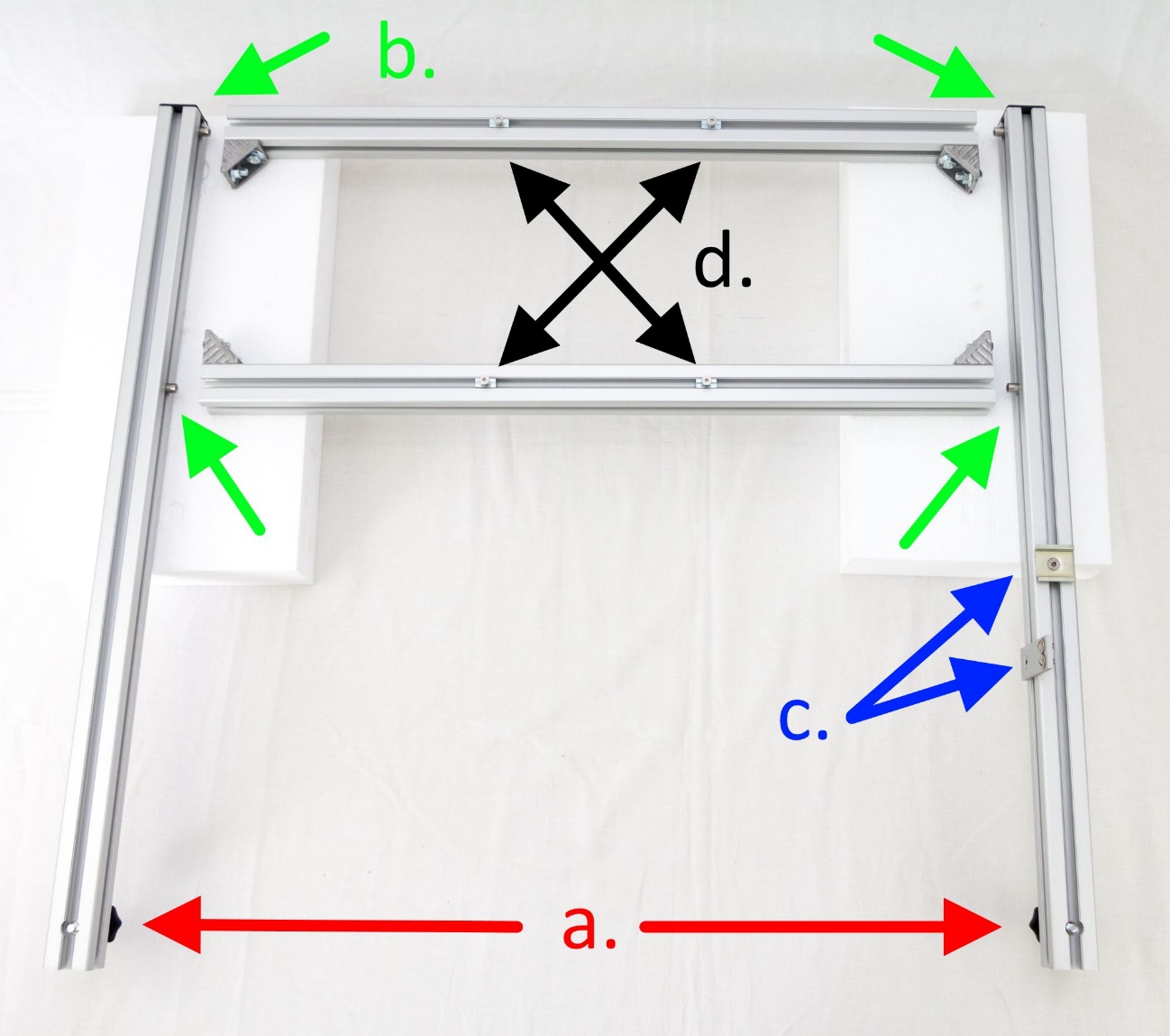
12. Feed the horizontal bars onto the guide bolts of the vertical bars. Mount the horizontal bars to the vertical bars by inserting M8-T-bolts with M8-nuts into the angle brackets and fix it.

    

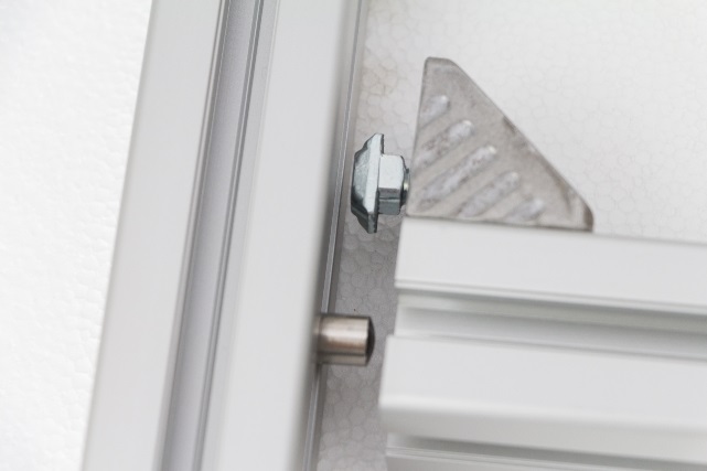
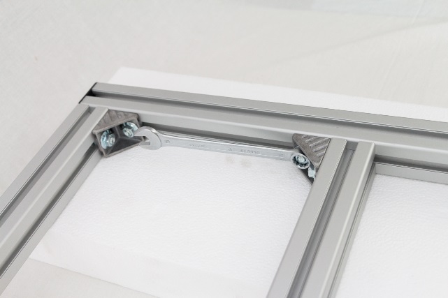
    (13 mm wrench needed)

Mounting the Z-axis frame to the bottom frame

13. Place the Z-axis frame on the ground frame and tighten the hand screws.

    

14. Insert the 45°-struts into the bottom- and Z-axis frame. Release the four hex socket screws until the T-nuts can rotate by 90° (turn it CCW). Then tighten the four hex socket screws (turn it CW).

    

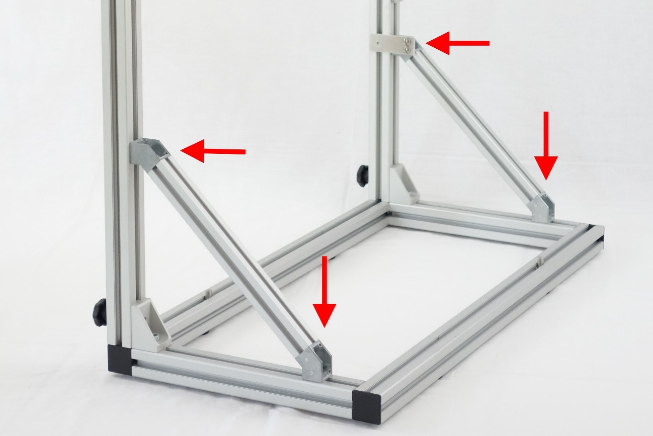
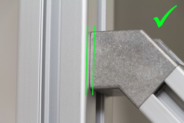
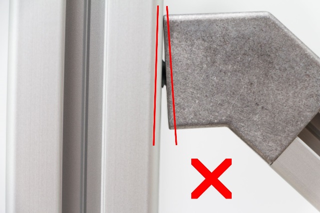
    Take care that the Z-axis frame is in right angle to the bottom frame.

    

Mounting the Turntable at the bottom frame

15. Mount the Turntable at the bottom frame. The connection panel at the Turntable must be positioned to the backside. The 45°-struts face to the front side.

    Insert the base struts of the Turntable into the guide bolts. Then the Turntable gets self-centered.

    

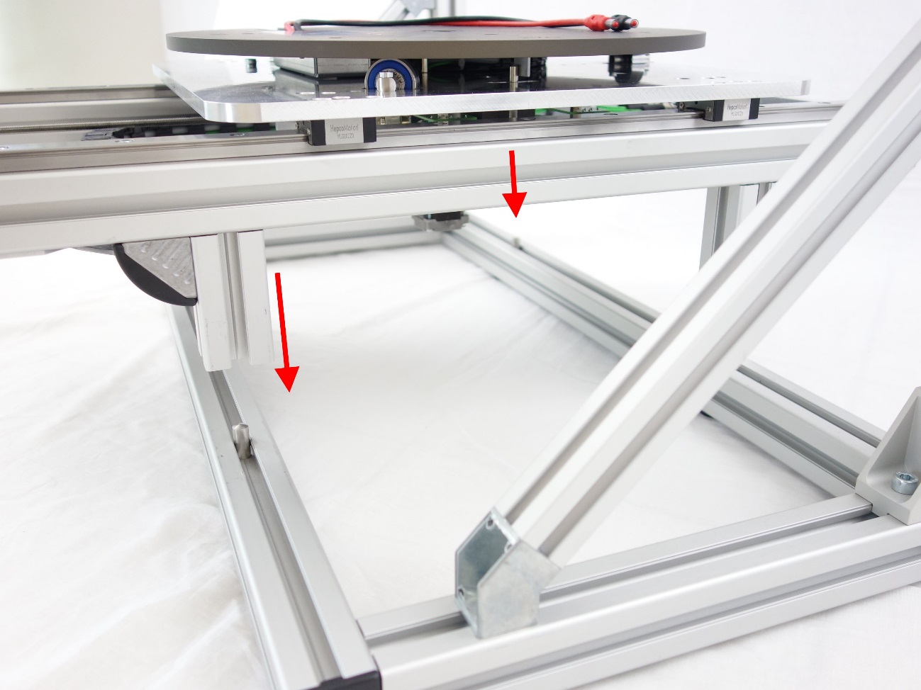
    Fix the Turntable by using the four angle brackets from step 3.

    

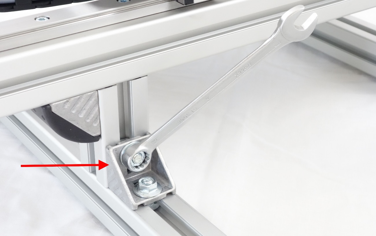
    (13 mm wrench needed)

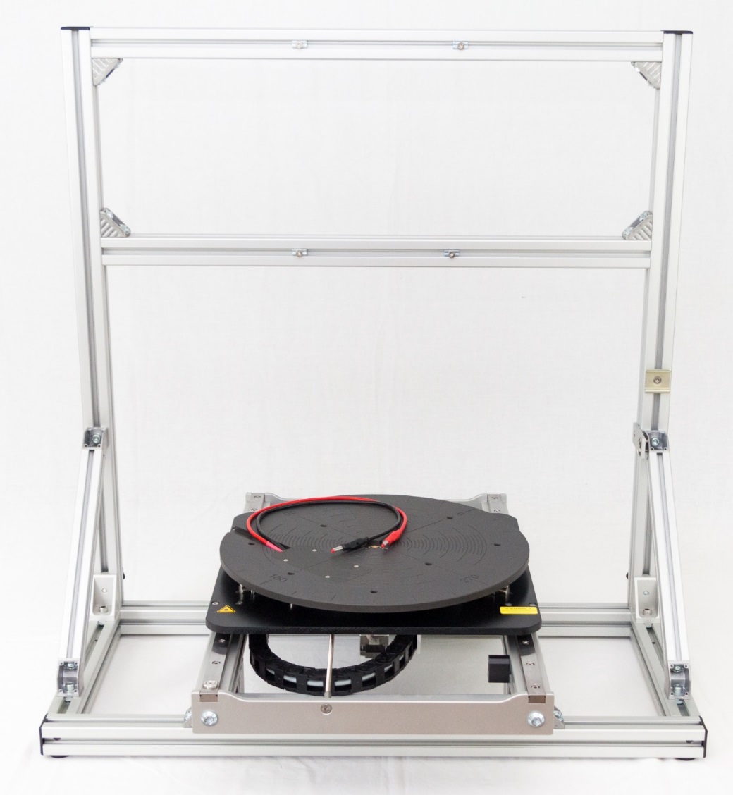
Mounting the Z-axis at the Z-axis frame

16. Remove the Z-axis shipping lock at the backside of the Z-Axis.

    

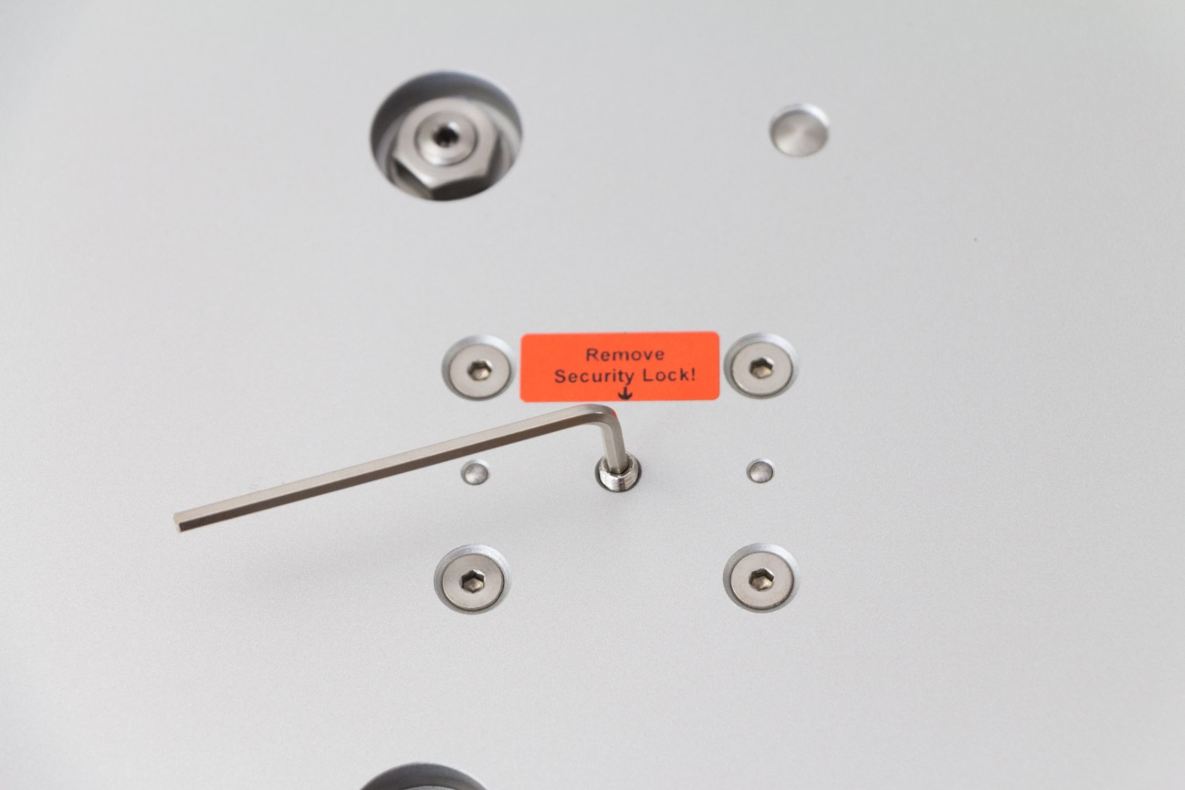
    (2.5mm hex-wrench needed)

17. Mount the Z-axis to the Z-axis frame by the usage of the four M5 hex countersunk screws, which are installed in the vertical bars.

    

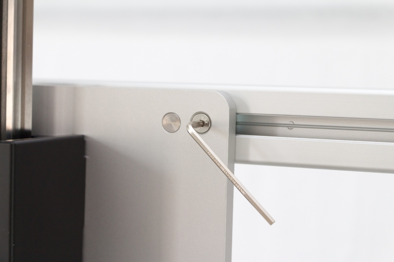
Mounting the cable chain to the Z-axis and the Z-axis frame

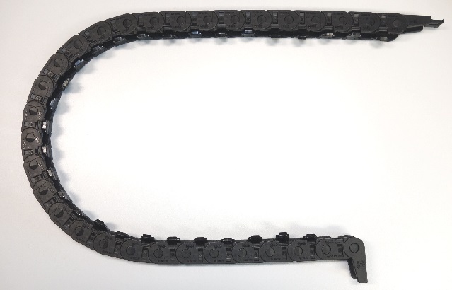
18. Open the cable chain. A slotted screwdriver should be used to open the clip at each chain link.

    

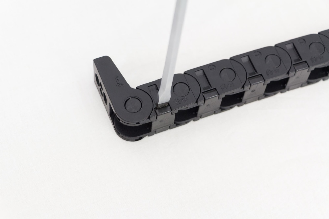
19. Mount the cable chain with its straight end piece at the cable chain holder at the right vertical bar.

    

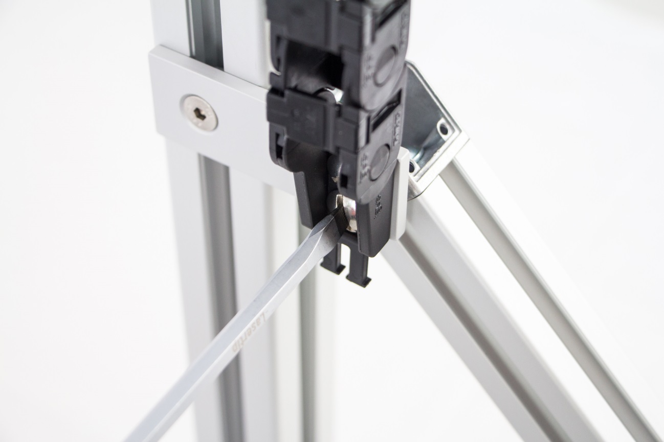
    (slotted screwdriver needed)

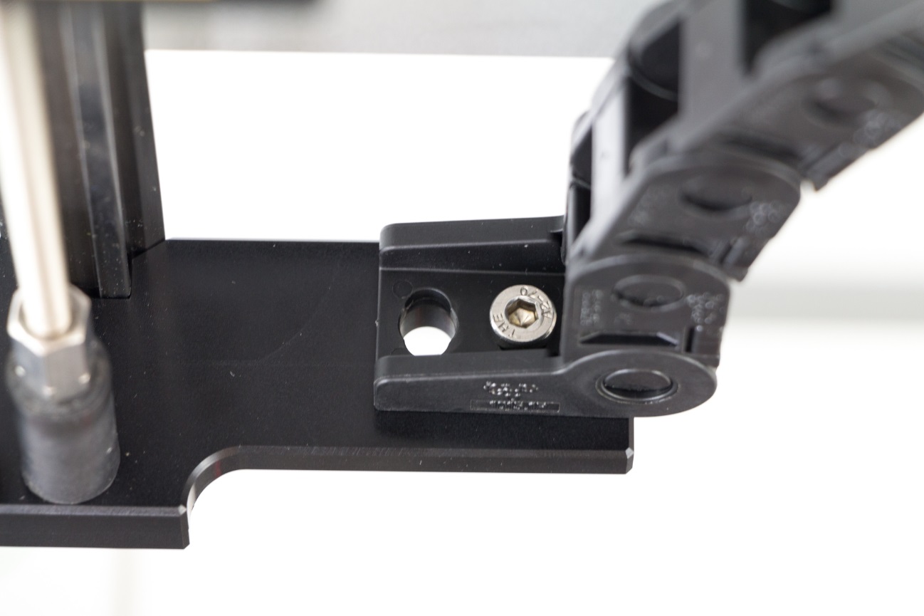
20. Remove the hex screw at lower end of the Z-axis.

    

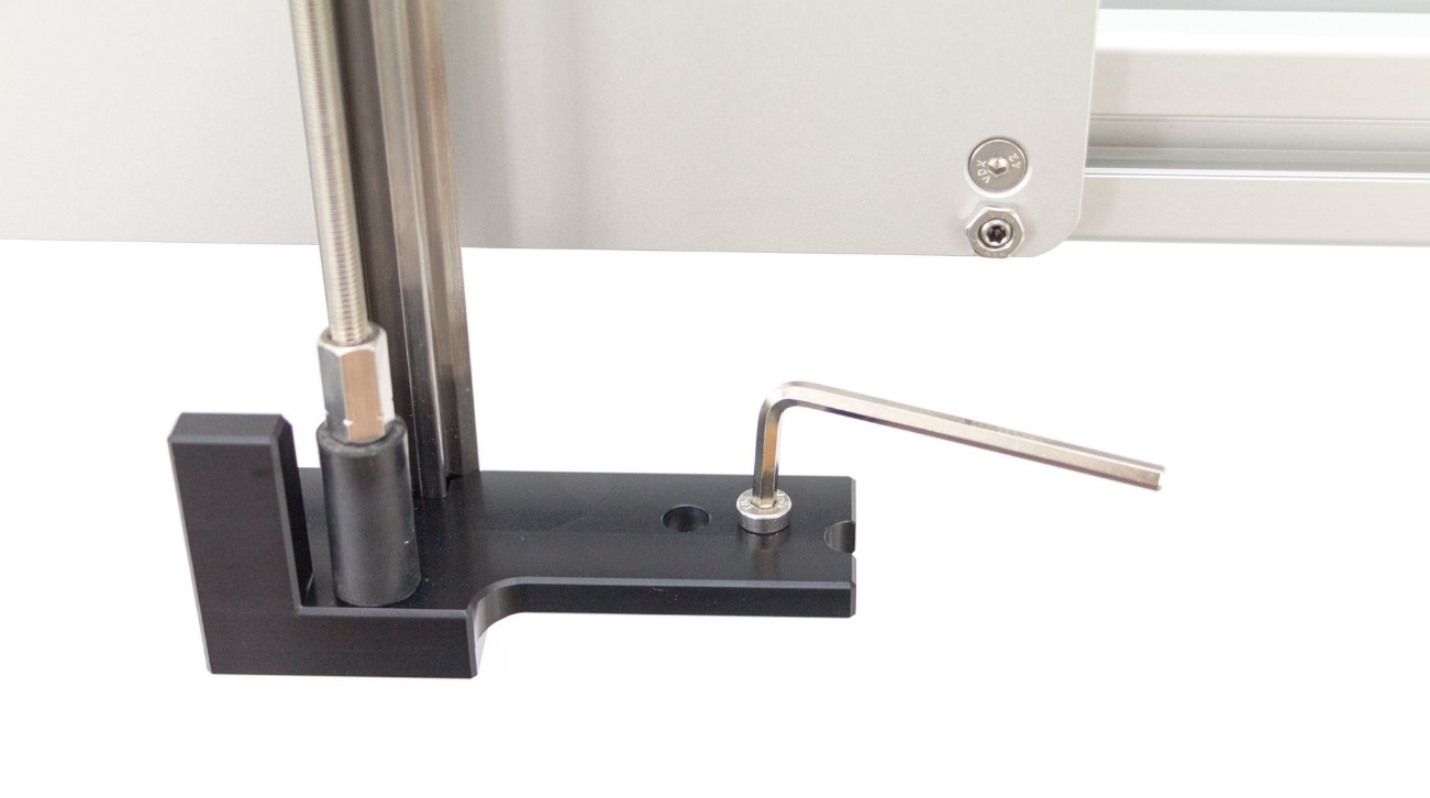
    (5 mm hex-wrench needed)

Mount the cable chain with its angled end piece at the lower end of the Z-axis.

Mounting the Laser head to the Z-axis

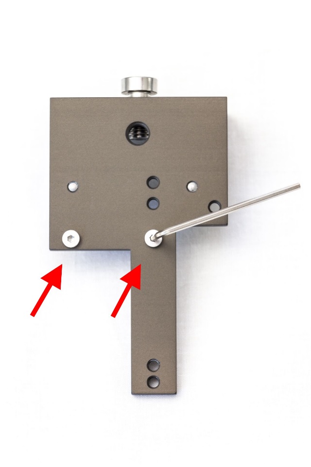
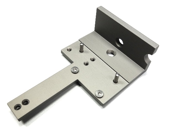
21. Remove the two M3 hex countersunk screws from the backside of the Laser Bracket.

    (2 mm hex-wrench needed)

    

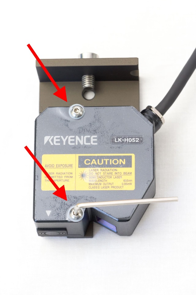
    Mount the Laser head to the Laser Bracket by the usage of two M4 x 38 mm hex screws and plastic washers.

    (2.5 mm hex-wrench needed)

22. Slide the Collision Sensor on the Laser head bottom-up. Use two M2.5 hex countersunk screws to fix it to the Laser Bracket.

    

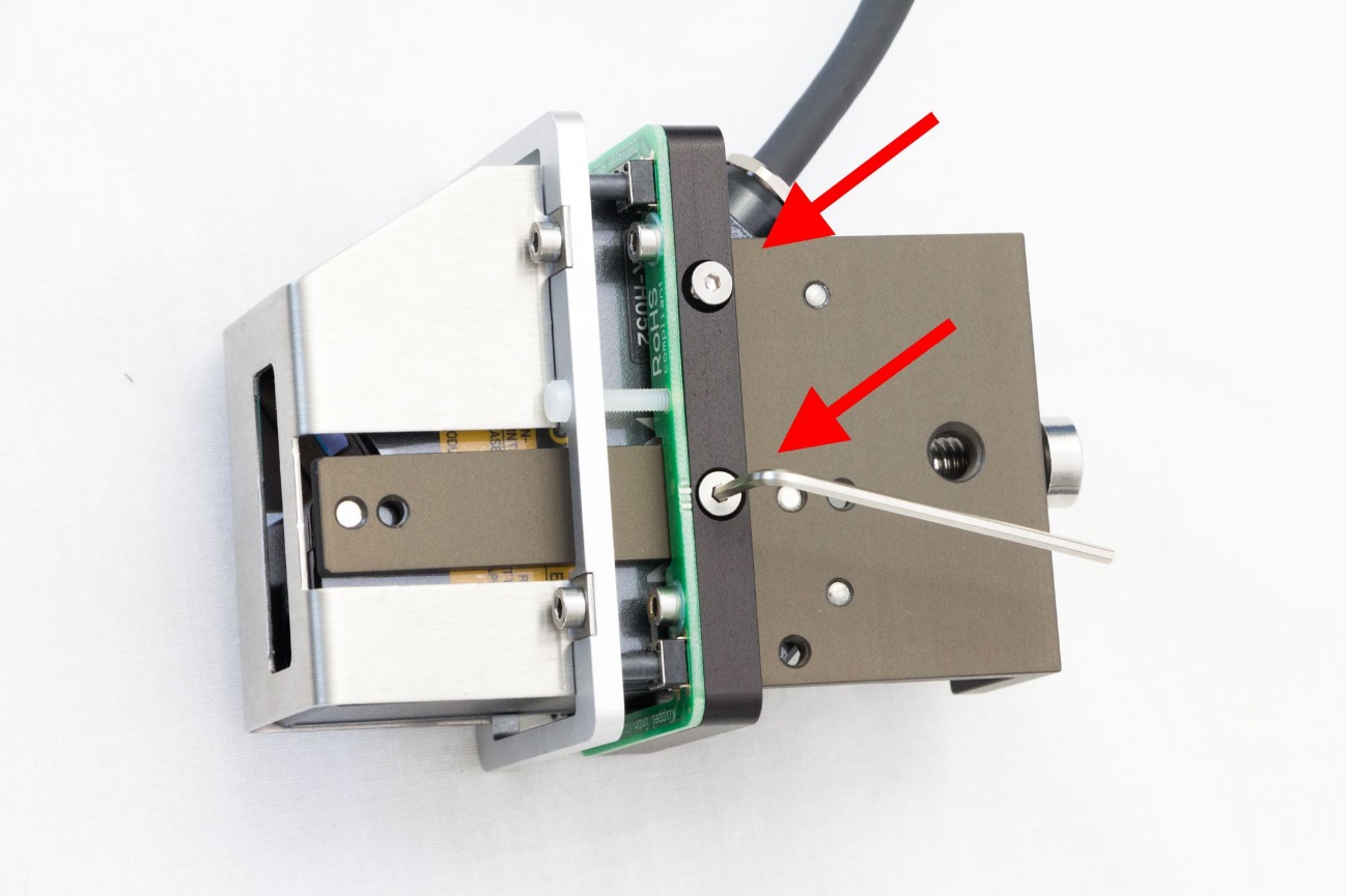
    (2 mm hex-wrench needed)

23. Mount the Laser Bracket with Laser head and Collision Sensor to the Z-axis.

    

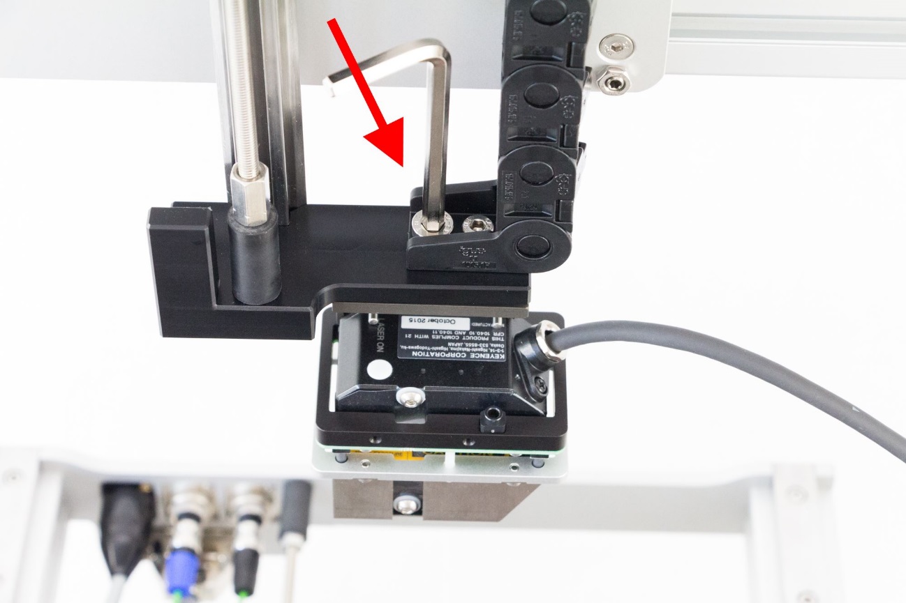
    (6 mm hex-wrench needed)

24. Connect the laser cable to the Laser head and the Collision Sensor Cable to the Collision Sensor.

    

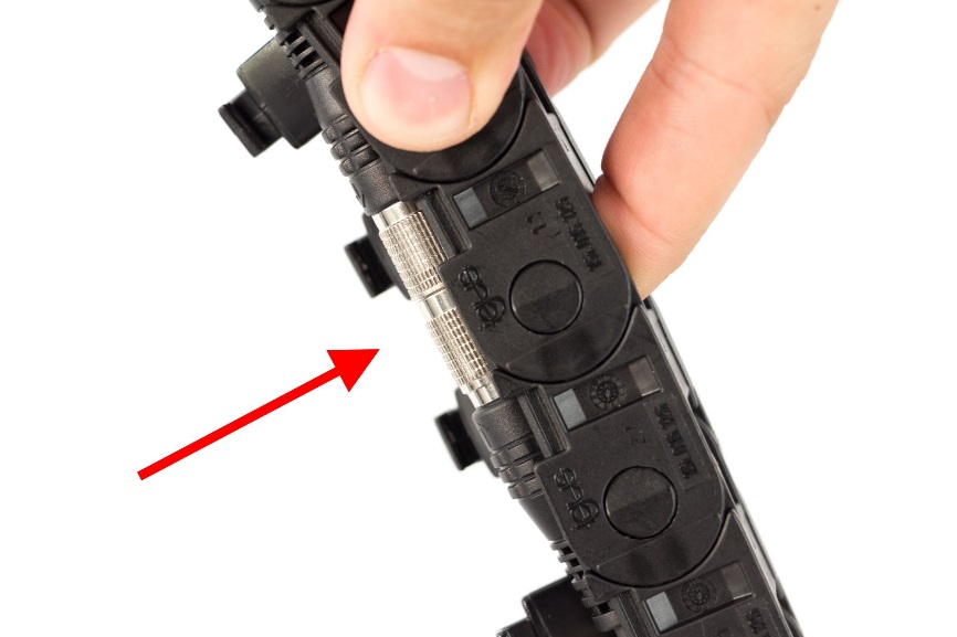
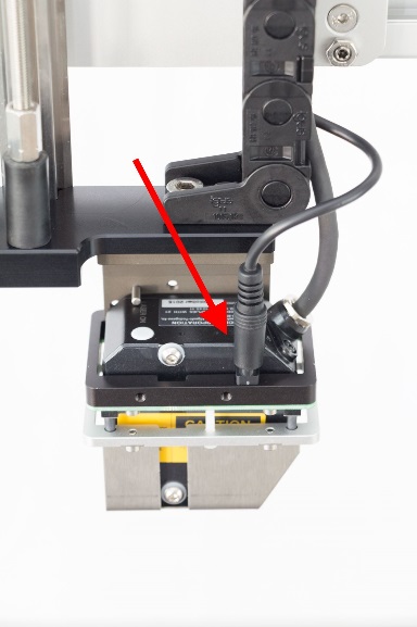
25. Insert both cables into the cable chain and close the clips.

Mounting of the Laser-Controller

26. Slide the Laser Controller sideward onto the holder clip on the right Z-axis vertical bar.

    Connect the Laser cable to Port 1 of the laser controller.

    

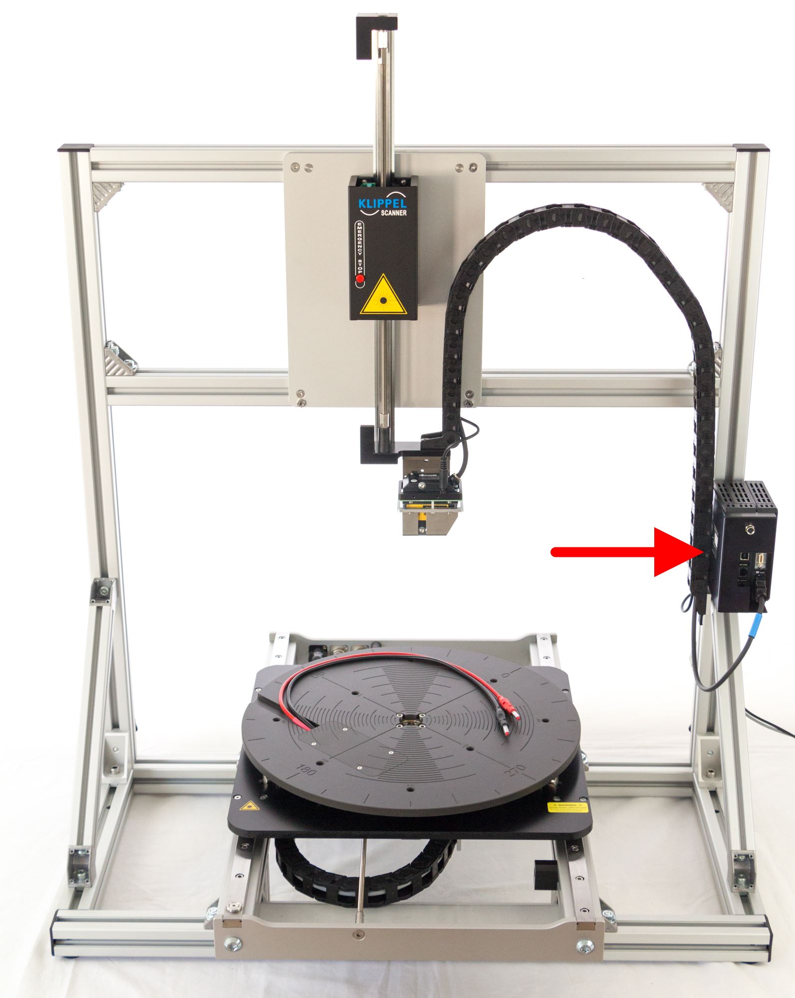
Finishing the Scanner Mounting

27. Connect the Z-axis cable to the Z-axis and install the cable at the backside of the frame.

    

    

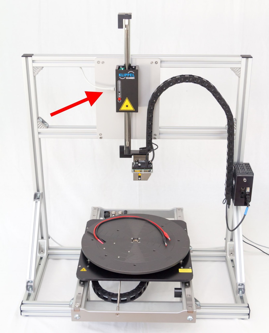
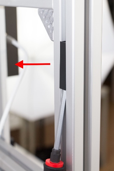
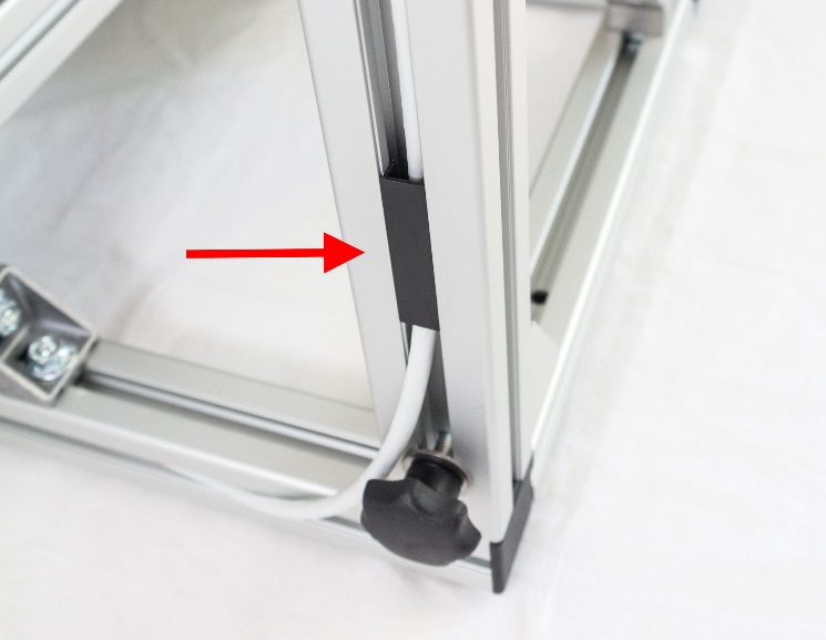
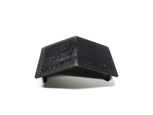
28. Snap on the plastic covers to the angle brackets.

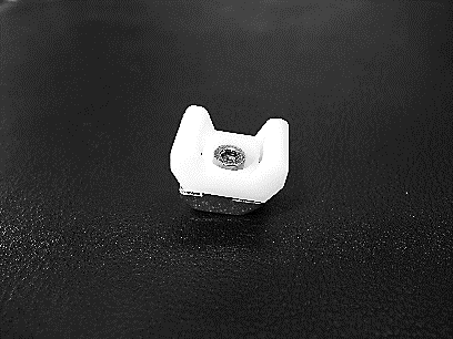
29. Mount the cable holder at the backside of the right vertical bar at 26cm above the ground.

    It should be used to fix all cables from the Laser Controller.

    

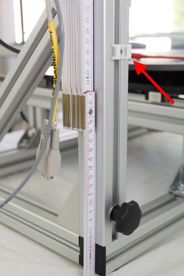
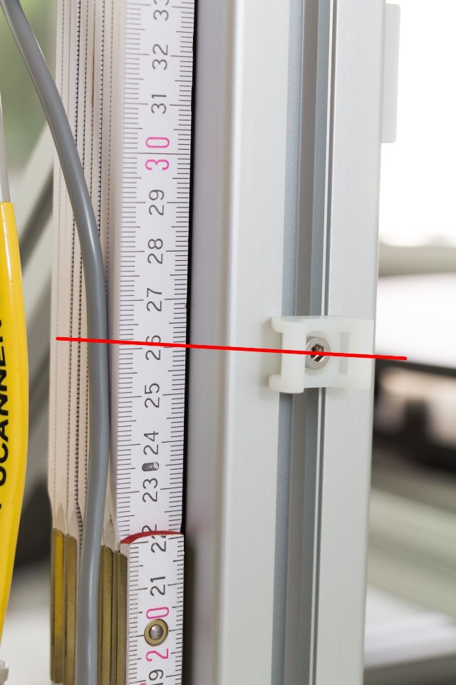
    (3 mm hex-wrench needed)

Please continue now with the Connection Setup

List of Parts

Turntable (pre mounted)

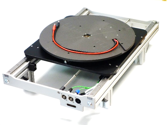
Z-axis (pre mounted)

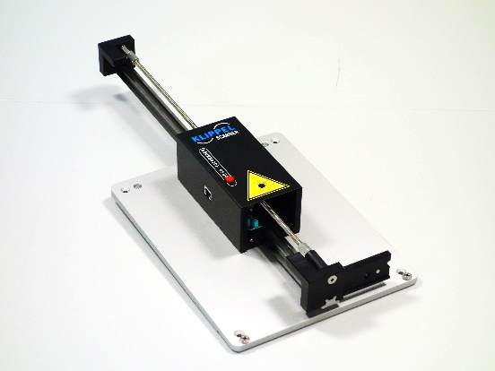
Bottom Frame (pre mounted)

• 8x M8-T-bolt

• 8x M8-nut

• 4x angle bracket

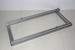
2x Vertical Bar

• 1x M8-hand-screw

• 2x guide-bolts

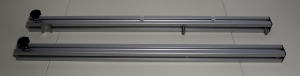
2x Horizontal Bar

• 4x M8-T-bolt

• 4x M8-nut

• 2x angle bracket

• 2x M5-T-nut

• 2x M5-hex-screw

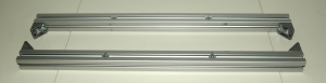
2x 45°-strut

• 2x M8-T-bolt

• 2x M8-hex-screw

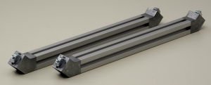
Angle Bracket Plastic Cover

• 8x big plastic cover for 90° angle bracket

• 4x small plastic cover for 45° angle bracket

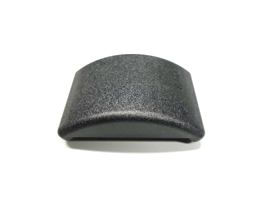
Cable Chain

Cable holder

6x Removable Cable Straps

SCN Laser Bracket (rev.304)

• 2x M3 hex countersunk hex screw

• M8 hex screw

Collision Sensor LK-H52 rev.1.1

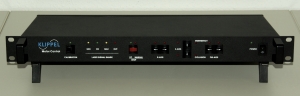
Motor Control

• Rev. 1.3 with M12 male 5 pin power socket

• Rev. 1.1 – 1.2 with M8 female 3 pin power socket

• Rev. 1.0 with DIN female 5 pin power socket

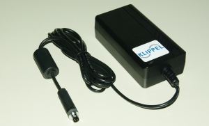
Motor Control Power Supply 24Vdc

with country specific main cable with M12 female 5 pin connector

• For MC rev. 1.1 -1.2 with adapter M12 male 5 pin to M8 male 3 pin

• For MC rev. 1.0 DA PSU with DIN male 5 pin connector needed

Speaker Clamp

• 2x cable Turntable to clamps (premounted)

• 2x small clamps

• 2x large clamps

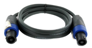
Speaker Cable 5m

SPEAKON to SPEAKON (Analyzer to Turntable)

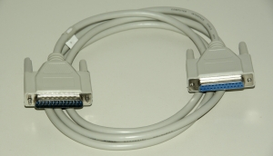
R-Phi-Axis Cable

D-Sub DB-25 shielded m/f (2m)

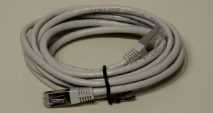
Z-Axis Cable

RJ45 shielded m/m (3m)

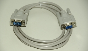
Laser Signal Range Cable

D-Sub DB-9 shielded m/f, (2m)

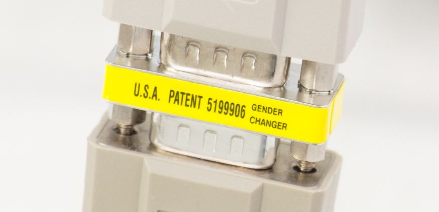
Laser Signal Range Adapter

D-Sub DB-9 m/f (screwable)

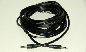
Collision Sensor Cable

3,5mm TRS Jack m/m (5m)

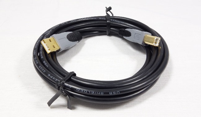
USB Cable 3m

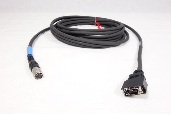
Laser Cable (0.7m)

Keyence Laser Sensor to Laser Controller

Centering Piece

• with rubber foam

• 1x M3-screw

• Small Calibration Cylinder

• Big Calibration Cylinder

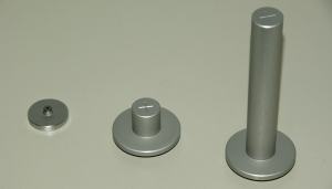
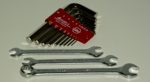
Tools

• Set of hex keys (2 to 8mm)

• 1x 13mm-wrench

• 2x 10mm-wrench

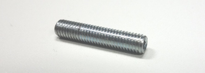
Z-Axis Shipping Lock

M5 bolt with inner hex collar

Phi-Axis Shipping Locks

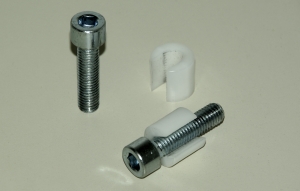
R-Axis Shipping Locks

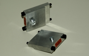
Connection Setup

The connection of all devices working together in the Klippel Scanning System needs to be done with care to assure the proper working of the Scanner. The steps correspond to the numbers in the Connection Illustration on the following page.

Some of the steps are already mentioned in the Mounting Instructions, so use the connection setup steps for checking and completing the scanner setup.

Scanner Hardware with Motor Control

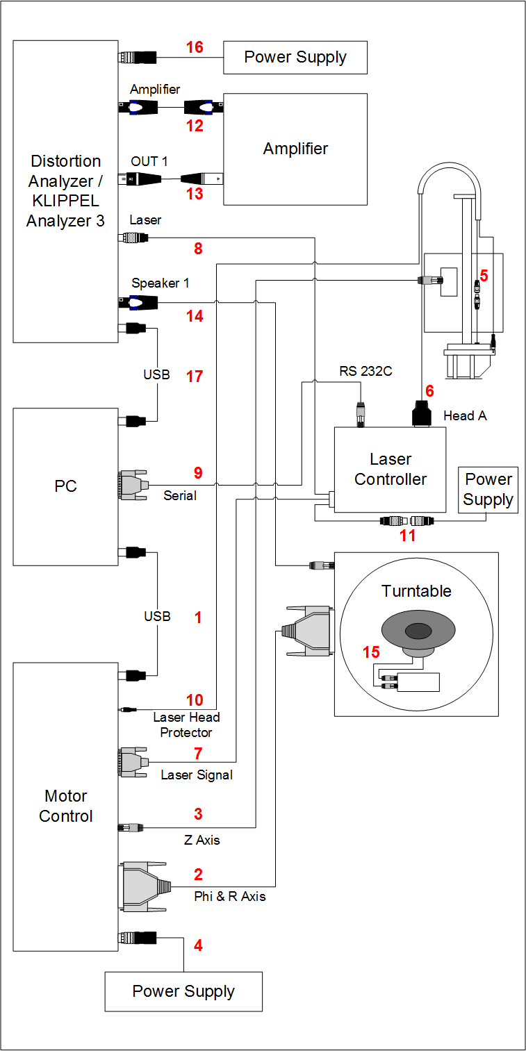
USB (1)

Connect the Motor Control to the PC with the provided USB-cord. (USB A – USB B)

Phi-R-Axis (2)

Connect the Motor Control to the Turntable with the provided Phi- & R-Axis-cord. Screw the connector together with the Motor Control! (D-Sub / DB-25 male - D-Sub / DB-25 female)

Note

The usage of shielded cables as delivered is required!

Z-Axis (3)

Connect the Motor Control to the Z-Axis with the provided Z-Axis-cord. Make sure that the plug is snapped in! (RJ 45 male – RJ 45 male)

Note

The usage of shielded cables as delivered is required!

PSU (4)

Connect the Motor Control with the provided 24V_DC power supply. Screw the connector together with the Motor Control for a good ground connection!

Motor Control rev. 1.1 – 1.2 with M8 female 3 pin socket could be used with 24V_DC PSU with M8 male 3 pin connector or 24V_DC PSU with M12 female 5 pin connector + M12 male 5 pin to M8 male 3 pin adapter.

Laser Controller Connections

Laser Signal digital (5)

Connect the Laser Head to the laser cable that is installed in the cable chain. Should still be done during hardware setup. (Keyence round screwable female)

Laser Signal digital (6)

Connect the laser cable to the port for Laser Head 1 at the Laser Controller. Should still be done during hardware setup. (Keyence rectangular snap-in male)

Laser Signal Range (7)

Connect the Laser Controller to the Motor Control with the Laser Signal Range cord.

At Keyence LK-G5001P Laser Controllers rev. >= 2.0, connect the Laser Signal Range cord directly to the socket named Laser Signal Range at Motor Control (D-Sub / DB-9 female) and at the Laser Controller (D-Sub / DB-9 male).

At all older Keyence Laser Controllers, connect Laser Signal Range cord with socket named Laser Signal Range at the Motor Control (D-Sub / DB-9 female) and with the short fixed mounted cord at the Laser Controller (D-Sub / DB-9 male). For a screwable connection, insert the Laser Signal Range Adapter between the Laser Controller cable outlet and the Laser Signal Range cable. (D-Sub / DB-9 male – D-Sub / DB-9 female cable & adapter)

Laser Signal analog (8)

At Keyence LK-G5001P Laser Controllers rev. >= 2.0, connect the Laser Controller to the Distortion Analyzer / KLIPPEL Analyzer 3 with the “Laser Supply & Signal” cord. (LEMO male 8 pin to M4 female 4 pin) Use “Laser 1” at the Laser Controller.

At all older Keyence Laser Controllers, connect the fixed mounted LEMO cord with the Laser input at the Distortion Analyzer / KLIPPEL Analyzer 3.

Note

The KLIPPEL Analyzer 3 has two laser inputs. Select the one in use in dB-Lab ‣ Hardware ‣ KA3 ‣ Signal Configuration

Laser Programming (9)

Connect the Laser Controller to the PC with the provided RJ12 to serial cord. The RJ12 plug has to be connected to the RS-232C socket of the Laser Controller, DB-9 to a serial port at the PC! (RJ12 male – D-Sub / DB-9 female, provided with the Laser Controller)

If PC doesn’t offer a serial port, add the provided USB-to-serial-adapter. (USB A male – D-Sub / DB-9 male)

A separate USB driver installation is needed on most systems.

Collision Sensor (10)

Connect the Laser Head Protector (Collision Sensor) to the Motor Control with the provided jack cord. The 3.5 mm TRS jack cord should still be installed in the cable chain. (3.5 mm TRS jack male - 3.5 mm TRS jack male)

Laser PSU (11)

Keyence LK-G5001P Laser Controllers rev. >= 2.0 could be powered directly by the KA3 via the “Laser Supply & Signal” (LEMO to M8 female 4 pin) cable. No external PSU is needed in this configuration.

Keyence LK-G5001P Laser Controllers rev. >= 2.0 connected to a DA2 need to be powered with a M12 male 5 pin to M8 female 4 pin “Laser Supply” cord connected to “Laser 2”.

All older Keyence Laser Controllers will be powered with an external 24V_DC PSU with M8 male 3 pin connector or external 24V_DC PSU with M12 female 5 pin connector + M12 male 5 pin to M8 male 3 pin adapter.

Note

Laser head has to be connected before powering the laser controller.

KLIPPEL Analyzer 3 (KA3), Amplifier and Loudspeaker

Amplifier OUT (12)

Connect the Amplifier Output to the KLIPPEL Analyzer 3 port Speaker-Card-AMP with a Speakon cord. (Speakon female – Speakon female or crimpled ferule – Speakon female)

KA3 XLR-Card-OUT1 (13

Connect the KLIPPEL Analyzer 3 port XLR-Card-OUT 1 to the Amplifier input with a XLR cord. (XLR male – XLR female)

KA3 Speaker-Card-SP 1 (14)

Connect the KLIPPEL Analyzer 3 port Speaker-Card-SP 1 to the Turntable with the provided Speakon to Speakon cord. (Speakon female – Speaonk female)

DUT at Turntable (15)

Connect the DUT to the speaker cables at the Turntable

KA3 POWER (16)

Connect the KLIPPEL Analyzer 3 to the provided power supply.

Screw the Connectors together for a secure ground connection! (M12 male 5 pin)

KA3 USB (17)

Connect the KLIPPEL Analyzer 3 to the PC with the provided USB cord. (USB A – USB B)

Distortion Analyzer (DA), Amplifier and Loudspeaker

Amplifier OUT (12)

Connect the Amplifier Output to the Distortion Analyzer port AMPLIFIER with a Speakon cord. (Speakon female – Speakon female or crimpled ferule – Speakon female)

DA OUT1 (13)

Connect the Distortion Analyzer port OUT 1 to the Amplifier Input with a XLR cord. (XLR male – XLR female)

DA SPEAKER 1 (14)

Connect the Distortion Analyzer port Speaker 1 to the Turntable with the provided Speakon to Speakon cord. (Speakon female – Speaonk female)

DUT at Turntable (15)

Connect the DUT to the speaker cables at the Turntable

DA PSU (16)

Connect the Distortion Analyzer to the provided power supply.

Screw the Connectors together for a secure ground connection! (DIN 5-pin male)

DA USB (17)

Connect the Distortion Analyzer to the PC with the provided USB cord. (USB A – USB B)

Security advice

Warning

Attention: Never use the Klippel RnD system at power sockets without EARTH connection!

The power supply for the Klippel Motor Control requires a protective earth conductor for proper operation. If the earth contact is removed it could cause high voltages at the enclosure of the device.

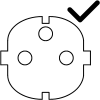
2 conductors + EARTH

2 conductors without EARTH

KLIPPEL GmbH takes no responsibility for any kind of damage or injury caused by improper or unspecified usage.

Warning

The Scanning Vibrometer hardware contains moving parts that are automatically controlled during operation. Make sure staff is not entering the working area during operation. Pay caution when setting up the device or during any other interaction with the machine.

First Calibration

The Scanner Hardware has to be exactly calibrated for measuring accurate scan data. Follow the subsequent calibration steps for a first calibration after any changes to the Scanner Hardware setup or after a new Software Installation.

1. Switch the Motor Control Device on. (Please switch it off first, if it was already switched on to reset the internal calibration.)

2. Start the Klippel Scanning System application.

3. Select the Perform Scan… entry from the File menu.

4. The Calibration dialog will appear to start the new Scanner Calibration

   

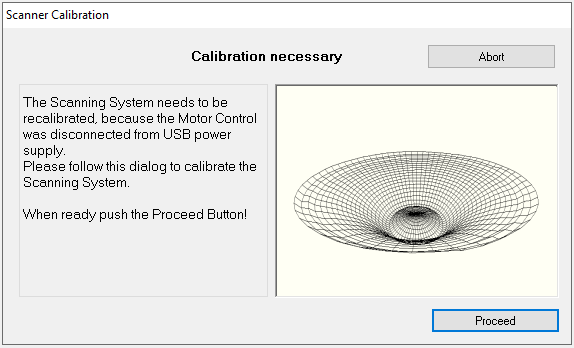
   Proceed to the next calibration step.

5. Please assure a safe operation of the Scanner Calibration. Any objects above and below the turntable are in danger of a collision with the calibrating laser. Proceed to the next calibration step.

   

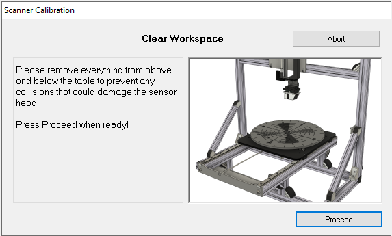
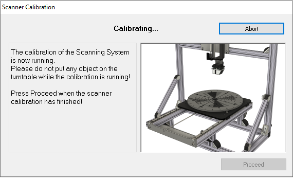
6. The Motor Control device approaches the end contacts of each movement axis. Proceed when the scanner calibration has finished.

   

7. Now the rest position of the turntable has to be set. This is very important to gain accurate scanning results.

   The turntable has to be adjusted exactly perpendicular to the Z Axis which moves the laser head up and down. Furthermore the laser beam should point exactly on the center of the turntable. That can be accomplished by using the two calibration cylinders.

   

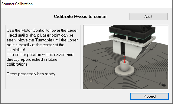
8. Insert the larger calibration cylinder into the slot in the center of the turntable. Move the laser head by using the hand controls at the Motor Control device until a sharp laser point can be seen on top of the calibration cylinder.

   Unfasten the four fastening screws and move the base plate of the Z-Axis for adjusting the lateral center position of the Scanner Hardware until the laser points at the center of the calibration cylinder.

   

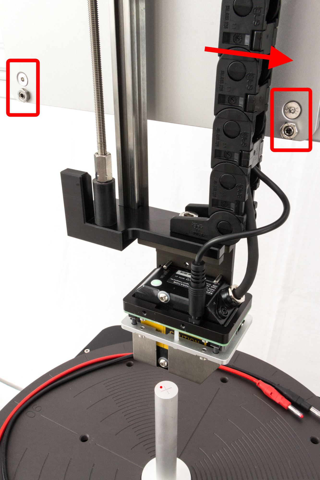
9. Use the Motor Control device to adjust the center position of the R Axis.

   

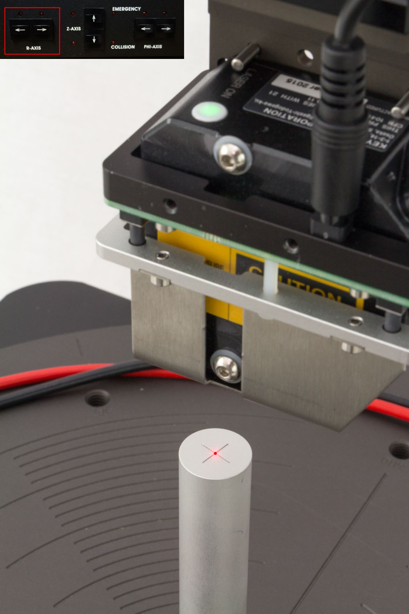
   To check the correct angle of the Z Axis the shorter calibration cylinder is helpful.

10. Remove the large calibration cylinder and put the shorter calibration cylinder into the slot on the turntable.

    If the laser spot deviates laterally from the center of the short calibration cylinder, then the laser head itself has to be realigned to point exactly downwards.

    

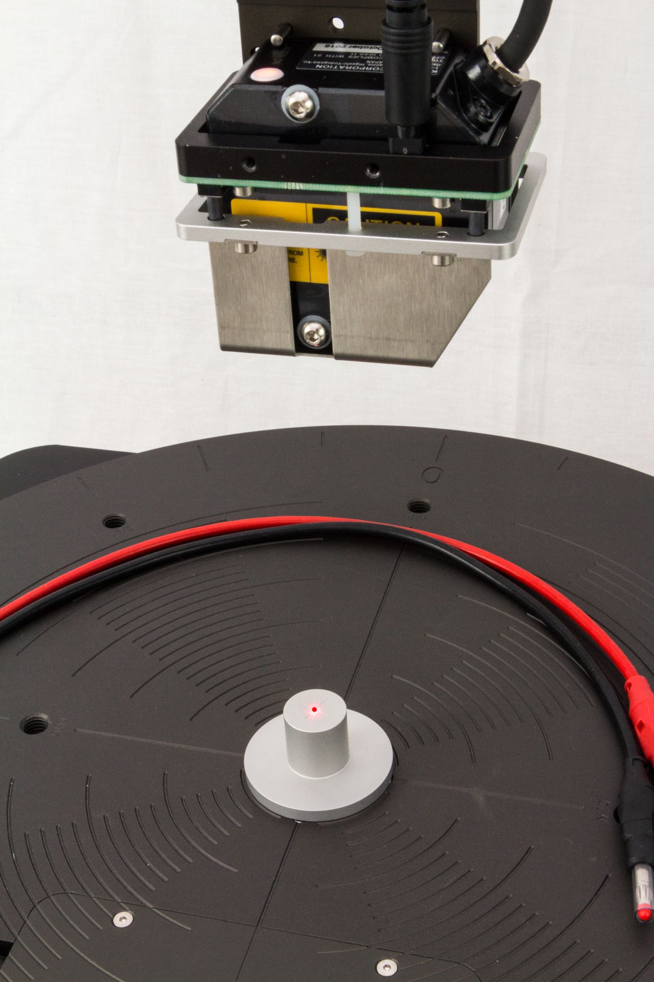
11. Move the laser head downwards by using the Motor Control device until a sharp laser point can be seen on the short calibration cylinder.

    A deviation of the laser point in direction of the R-Axis indicates a tilting of the Z-Axis base plate. The distance between the laser point and the center of the calibration cylinder \(\Delta r\) times 6 shows the root point \(M\) where the laser beam is perfectly perpendicular to the turntable.

    

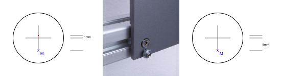
    Loose the counter nuts for the adjustment screws at the Z Axis base plate and turn both adjustment screws until the laser points on the root point \(M\). Now use the Motor Control device to adjust again the center on the calibration cylinder in R direction.

    

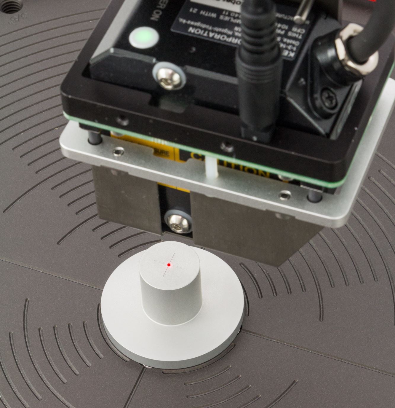
12. Fasten the Z-Axis base plate again with the four fastening screws and check again the correct centering of the larger calibration cylinder.

    If the centering has been successful then Proceed with the Scanner Calibration Dialog of the Klippel Scanning System.

    

    Now the Scanner Hardware is calibrated and can be safely used.

SCN Tutorial

What is the goal of this tutorial?

This tutorial makes you familiar with the SCN module.

1. In Tutorial 1 – Viewing SCN Results we will show you how to view already measured SCN results.

2. The following Tutorial 2 – Performing a Scan provides a step by step recipe to conduct a laser vibration measurement on a loudspeaker cone.

3. In the next Tutorial 3 – Customizing SCN we discuss modifications of the scanning setup parameters to use more powerful features and gain vibration results of higher quality and information content.

4. The Tutorial 4 – Radiation Area SD is dedicated to the measurement of the effective radiation area S_D. You can learn how to determine an accurate S_D from measured SCN results and how to optimize the scanning setup for S_D scans.

To perform own vibration scans the Klippel Scanner Hardware and appropriate software licenses are required.

Tutorial 1 – Viewing SCN Results

The Tutorial 1 gives a quick guide how to view already measured SNC vibration scan data.

Open a Scan

Start the Klippel Scanning System Application.

1. Open a Klippel Scanner Project File .ksp by using the menu entry File ‣ Open Scan…

   Example scans can be found in the ScanData Folder of your Scanning System Installation or on the Installation CD.

Klippel Scanner Project Files .ksp can also be opened by Double-click from the Windows Explorer

The scan data is loaded from the file and after execution of several post-processing scripts the data will be visualized.

The main surface of the Klippel Scanning System is divided into three analysis tabs in the upper part of the application window.

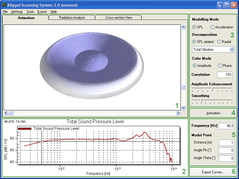
2. Select the following Settings (3):

   • Modelling Mode: SPL

   • Decomposition: SPL related Total Vibration

   • Color Mode: Amplitude

   • Correlation: 10%

   • Amplitude Enhancement: 0 dB (center)

   • Smoothing: 2

3. Start the 3D animation with the Animation Button (4).

4. Select a different analysis frequency by clicking into the Total SPL Plot (2).

5. Stop the 3D animation again using the Animation Button (4).

Improve visual quality

1. Set the Correlation to 0% and the Smoothing to 0. Now only the pure measurement data is visualized. Some measurement points might be noisy and show incorrect vibrations of high amplitude.

2. Increase the Correlation until most of the obviously erroneous measurement points are removed. Recommended Correlation values range from about 10% for good scans up to 95% for very noisy scans. Remaining invalid erroneous points can also be removed manually by marking them as corrupted in the Cross-sectional Cut.

3. Set the Smoothing again to level 2 or 3 to further reduce the noise in the scan data visualization.

4. Go to the menu entry Settings ‣ Preferences

   

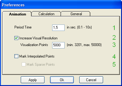
5. Select the following Animation Preferences and confirm with Ok:

   • Period Time (1): 1.5

   • Increase Visual Resolution (2): Checked

   • Visualization Points (3): 5000

   • Mark Interpolated Points (4): Checked

   • Mark Sparse Points (5): Unchecked

   Now there will be additional points interpolated in between the measurement points.

6. Go again to the menu entry Settings ‣ Preferences by pressing the F2 key.

7. Uncheck the option Mark Interpolated Points (4) to use the actual interpolated point color for the 3D Animation.

8. Shift the 3D Animation by clicking with the left Mouse button on it and dragging the Mouse up and down. Shift the position of the 3D Animation up and down by dragging with the mid Mouse button.

You can Reset the 3D view to standard values by the context menu which appears with a right Mouse click on the 3D Animation.

Tutorial 2 – Performing a Scan

In Tutorial 2 a quick guide is given, how to conduct own vibration scans with the Klippel Scanning System.

You will need the complete Klippel Scanner Hardware and TRF Measurement Licences to conduct own vibration scans!

Start new Scan

1. A new vibration scan can be started, provided that the Klippel Scanner Hardware is connected properly, see section Setup of the Scanning System for detailed instructions.

2. The setup of a new scan can be started by selecting Perform scan… in the File menu of the Klippel Scanning System.

If the option Perform scan… is missing in the File menu, you need to Enable the Scanning first in the General Preferences!

If several instances of the Klippel Scanning System application are running at the same time, only the first opened application is capable to connect to the Motor Control device and to perform scans.

Startup Scanning

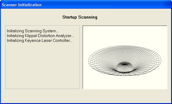
Before a new scan can be started, some automatic initialization procedures are run to test the proper connection of the Klippel Analyzer hardware, the Keyence Laser Controller and the Scanner Hardware. See the Initialization Reference for a detailed description of the initialization steps.

Scanner Calibration

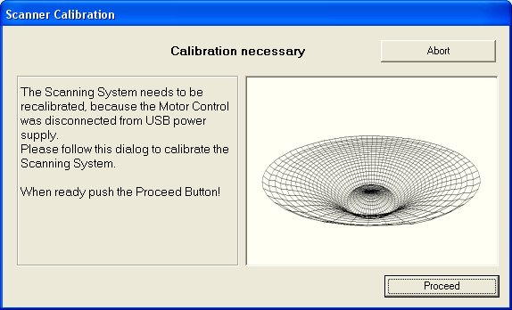
The Scanner Hardware needs to be calibrated each time when the Motor Control has been switched off or disconnected from the PC.

Follow the calibration steps to complete the calibration. See Motor Control Calibration Reference for a detailed description of the calibration steps.

Start new Project

After the initialization steps a new scanning project can be started.

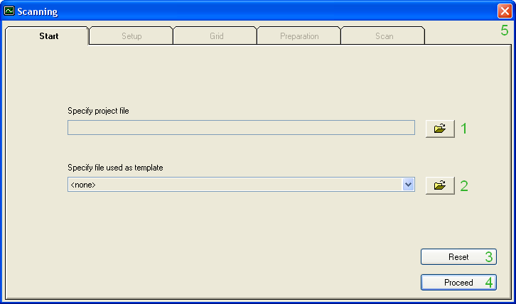
1. Click on the Button (1) and specify a new scanning project file.

2. Proceed (4) to the General Scan Setup

General Scan Setup

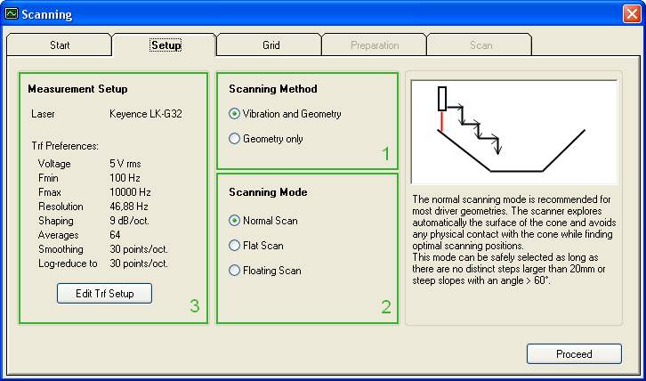
Leave the Scan Setup as it is preset and Proceed to the Measurement Grid Setup.

More information about the General Scan Setup can be found in the Reference.

Measurement Grid

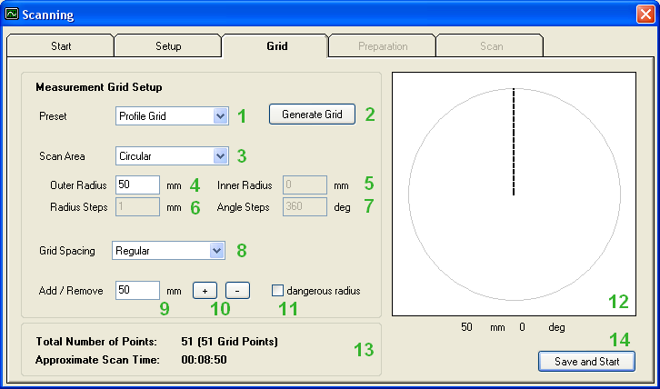
1. Choose the Profile Grid Preset (1) to measure a single cross-section line.

2. Enter the Outer Radius (4) of your driver and press the Generate Grid (2) Button.

3. Press the Save and Start (14) button.

A scan of a profile line provides already a quite good picture of the vibration properties of the loudspeaker in very short time (less than 10minutes).

It is possible to influence the Measurement Grid further by selecting a Manual Grid Preset (1), see the section Measurement Grid in the Reference for more details.

Start Scanning

You need to follow the Scan Preparation steps before the automatic Scanning Process can start.

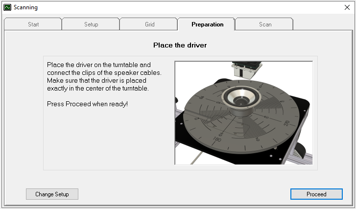
Each Preparation Step is described shortly next to an illustrating picture. See the Reference for the Scan Preparation steps for a detailed explanation of all steps.

1. Place the driver

   • Proceed

2. Find highest point

   • Approach the highest driver point by using the Motor Control device and Proceed

3. Check correct laser position

   • Proceed to start the Scanning

The scanning runs fully automatically and measures the loudspeaker vibration each point of the defined Measurement Grid.

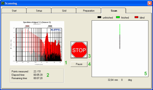
In the Grid Picture (5) the current progress of the scanning can be observed and the Remaining Time (2) for the scan is shown.

When the scanning process has finished the results can be visualized, see section Review and Analyze Scans.

Pause scan and resume

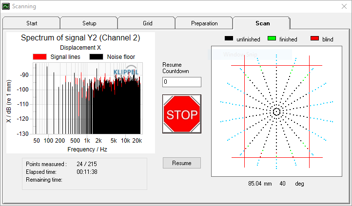
During the scan the measurement can be stopped or paused at any time. In addition there is the option to delay the resume by using Resume Countdown. This can be used to start a scan at a specific time for example when all coworkers has left the lab in the evening.

Tutorial 3 – Customizing SCN

The Scanning System offers a variety of options for optimizing the output from loudspeaker scans. This tutorial shows how to find good setups to use the Scanning System in an efficient way.

Fast Scanning

Several points need to be considered for finding a scanning setup which is adequate for the respective task and can be finished in minimal scan time.

The automatic vibration scanning can become quite time consuming for extensive grids. Therefore it is worth thinking about the required grid resolution before starting the scan.

1. Start a new Scanning Project as described in Tutorial 2 – Performing a Scan and proceed to the Measurement Grid Setup.

   

   We recommend scanning a loudspeaker at first in a Profile Grid (1).

   The Profile Grid sets 51 equally spaced grid points along one line from the center of the speaker to the outer radius. That type of scanning grid takes less than 10 minutes of scan time and you already get a good picture of the radial vibration behavior of the cone.

No asymmetric vibration behavior can be seen in a profile measurement!

2. Switch the Grid Preset (1) to a Manual Grid. Now a finer influence on the measurement grid is possible.

3. Change the Radius Steps (6) to a smaller value and press Enter. You can see how changing the number of grid points affects the Approximate Scan Time (13).

4. By selecting the Profile Grid Preset (1) again, all manual adjustments of the grid are discarded.

5. Go back to the General Scan Setup by clicking on the Setup tab and open the TRF Setup.

   

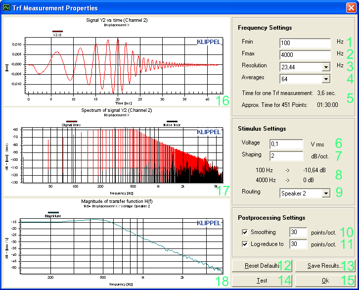
   Here you can also see the Approximate Scan Time (5) for the current Setup.

6. Set the number of Averages (4) to 1 (Single) to switch off the averaging. Now the scanning is faster, but the signal-to-noise ratio of the measurements gets very poor. A number of 64 averages has approved as a good compromise between scan time and scan quality. If the time is not as important, you can increase the number of averages to 128 or even 256.

7. Select a Frequency Resolution (3) of 0.73 Hz. Now the scanning time increases dramatically because each single TRF measurement takes much more time.

   Also the size of the data file and the calculation time of the post-processing operation will increase for higher frequency resolutions. That can be avoided by Log-reduce (11) the frequency axis afterwards. Then only the logarithmically reduced result curves will be saved.

   The application of Smoothing (10) and Log-reduce (11) has also an averaging effect in the frequency domain. If they are both enabled, then a higher Frequency Resolution (3) will lead to a better signal-to-noise ratio especially at high frequencies. Therefore the number of Averages (4) can be reduced again to 32 or 16 for higher frequency resolutions and the measurement time can be shorter.

   Recommended Frequency Resolutions range from about 5.86Hz to 46.88Hz.

8. Close the TRF Measurement Properties and switch the Scanning Mode (2) to Flat Scan.

   

   In the Flat Scan driving mode the position of the Z-Axis will not be changed. This is useful for rather flat driver geometries like for example micro speakers where the distance between the highest and the lowest measurement height is less than the focal range of the laser head.

   Then the laser head does not have to be moved up and down to adjust the measurement distance to the driver, which speeds up the scanning process considerably.

Tips for Scanning difficult drivers

Cone surface reflective or (semi-)transparent

Use some kind of surface coating to increase the diffuse reflectivity and improve the quality of the measurement data.

Very light-weight drivers

Fix the driver with modeling clay or a non-magnetic clamping to prevent the driver from moving during the scanning process. For small speakers and microspeakers, we recommend to use the Klippel microspeaker stand.

Oval or rectangular driver shape

Align the driver with its longer axis along the R-Axis of the turntable.

Consider using a Flat or Floating Scanning Mode in the General Scan Setup to increase measurement speed.

Apply a Rectangular Scan Area to the Measurement Grid.

High steps or gaps in driver geometry

Define a Dangerous Radius in General Scan Setup where the obstacle is situated on the cone.

Make a supervised profile scan first, to assure a safe overcome of the obstacle.

Consider using a Flat or Floating Scanning Mode in the General Scan Setup to increase measurement speed and robustness.

Non-vibrating dust cap in center (phase plug)

Enter an Inner Radius for the Measurement Grid to scan only the vibrating cone region.

Noisy measurement data

Use some kind of surface coating to increase the diffuse reflectivity and improve the quality of the measurement data.

Adapt the TRF Setup by increasing the voltage of the stimulus or making more averages.

Try to get a signal-to-noise ratio of at least 20dB in the desired frequency range.

Be aware, if the driver does not move at the current scanning point / frequency, then you can only measure noise.

Tutorial 4 – Radiation Area SD

The Radiation Area SD can be calculated based on the measured scanning results. An accurate result for the effective radiation area can be obtained, particularly for small drivers and asymmetric driver shapes.

This tutorial shows how to use the S_D calculation tool and how to find good scanning setups in order to achieve accurate results for S_D.

Calculating the Radiation Area SD

The effective radiation area S_D can be calculated for all measured loudspeaker scans.

You will need separate Licences for the S_D calculation for your own vibration scans!

1. Open a Scanner Project File *.ksp by using the entry File ‣ Open Scan…

   Example scans can be found in the ‘ScanData’ Folder of your Scanning System installation or on the installation CD.

2. Click in the menu-bar on Tools ‣ SD Calculation. Now the S_D calculation window will appear.

3. Set a suitable averaging radius:

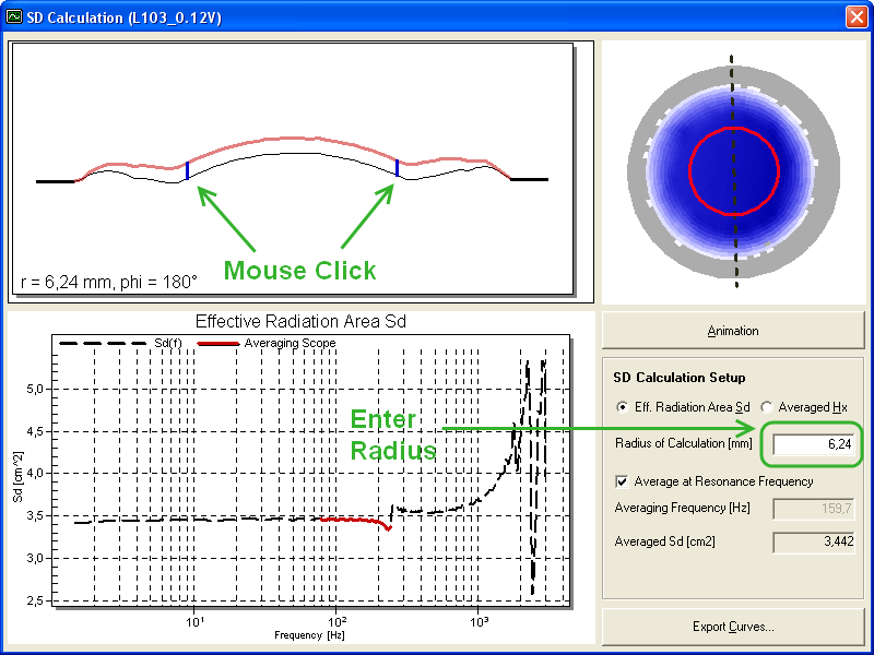
The selected averaging radius should be within the voice coil radius, where the driver moves with an equally high and representative excursion (piston mode). If the speaker is rectangular, set the radius smaller than the radius of the narrow side of the speaker.

Click in the cross sectional cut or if known enter an averaging radius in the respective text input field

The vibrations in the Cross-sectional Cut and the Amplitude Distribution plot will refer to the frequency which is selected in the main application.

4. Set a suitable averaging frequency:

   By default the averaging frequency is set at the estimated resonance frequency of the measured driver (maximum of velocity).

   The averaging scope is marked red.

   

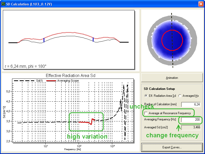   If the red averaging scope contains larger variations of the S_D(f)-graph, decrease the averaging frequency to place the averaging scope to the flat plateau of the graph.

   

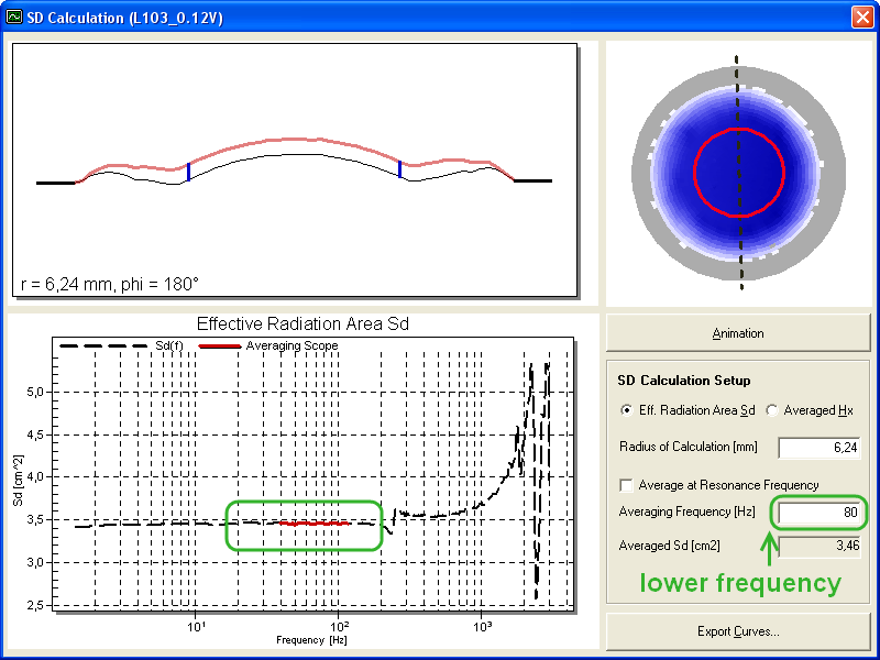   Uncheck the checkbox Average at Resonance Frequency and enter a smaller Averaging Frequency.

Troubleshooting

Big Variation of SD – value by changing ravg

Insufficient SNR

• Increase voltage of stimulus

• Decrease shaping to improve SNR at low frequencies

• Check reflectivity of surface (apply surface coating)

Bad measurement point distribution

• Increase grid resolution of measurement points

Strong bending modes in low frequency range

• Decrease Averaging frequency

Early SD(f) variation in graph

Asymmetrical rocking and bending modes

• Decrease Averaging frequency

5. View the Hx-displacement Curve:

   

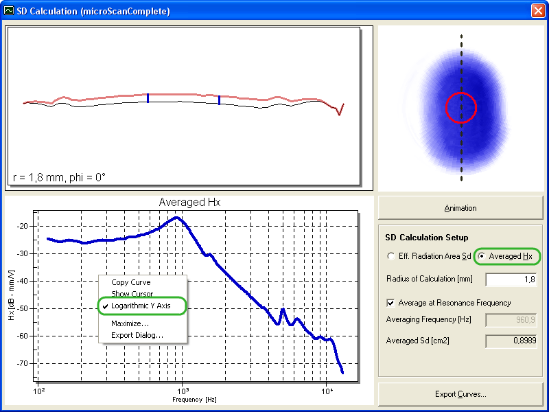   Select Averaged Hx (option button).

   Via the popup menu of the Averaged Hx Chart it can be switched between a Linear and Logarithmic Y Axis scaling.

   Choose an averaging radius within the voice coil to obtain representative data.

In the center of the cone (r = 0mm) there is only one actually measured point and an averaging of Hx cannot be applied.

See also the Reference section for calculating the Effective Radiation Area SD.

Measuring and Determining S_D

Here is described how to set up a vibration scan which is optimal for determining the S_D of a loudspeaker.

1. Start a new Scanning Project as described in Tutorial 2 – Performing a Scan and go to Setup.

   Regarding to the shape of the cone check if you can set the scanning mode to Flat scan, since many multimedia speakers, headphones and microspeakers have a relatively plane cone shape.
2. Now edit the TRF Setup (stimulus properties).

   The stimulus properties have to be set to a preferably high signal-to-noise ratio in the range where the parameter S_D will be determined, preferably around the resonance frequency of the driver.

   Depending on the speaker and its resonance frequency fs the minimum frequency range Fmin of the stimulus should begin below 1/4^th of fs and go up to Fmax at least 4 times fs.

   

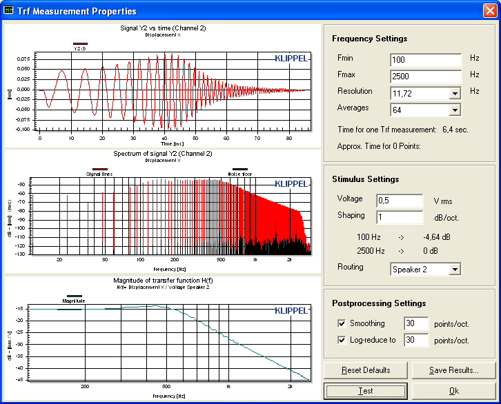   A sufficiently dense frequency Resolution is required to obtain an accurate S_D value. Depending on Fmin and the resonance frequency of the driver the frequency resolution should be set to 23.44Hz at the maximum. If the measurement time is less critical, a resolution of 5.86Hz or lower is recommended.

   It is recommended to use the Postprocessing Setting Log-reduce to 30 points per octave to reduce the final frequency resolution for higher frequencies. That helps keeping the final data file size low and allows to select higher resolutions for more accurate results at low frequencies where S_D is determined.

   The smaller the speaker (microspeaker) the more important is a high number of Averages, so that 32 to 64 Averages are recommended.

   To accomplish a high signal-to-noise ratio in the low frequency range the Shaping of the stimulus can be very low or even zero. But then the adjustment of the Voltage has to be done with caution to avoid damaging the driver by too high voltages!
3. Proceed with the Measurement Grid Setup.

   The SD Grid Preset (1) is a good compromise between a sufficient grid resolution and moderate scanning time.

   

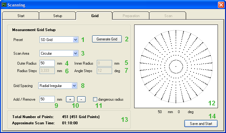   For a Circular Scan Area [3] it is recommended to apply a Radial Irregular Grid Spacing [8], which places measurement points with an increasing radial distribution with growing radius. Therefore the area of the surround which shows more intricate vibration behavior has a higher resolution.

   The Outer Radius [4] of the measurement has to be set large enough to cover the complete vibrating cone area in order to obtain a correct S_D value. It is recommended to set the outer radius a bit larger than the outer radius of the surround and to cover i.e. a small portion of the non-vibrating frame of the driver.

   

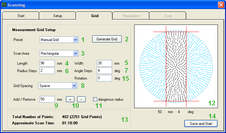   For a Rectangular Scan Area [3] it is recommended to apply a Sparse Grid Spacing [8] instead, which places measurement points more uniformly all over the scanning area.

   Depending on the actual Length [4] and Width [5] of the scan area it is possible to adjust the Radius Steps [6] and Angle Steps [7] in an Manual Grid Preset [1] to achieve a good coverage of the scan area.

   A number of about 400 Total Points [13] is sufficient for obtaining an accurate S_D.

4. Start the scanning now as described in Tutorial 2 – Performing a Scan

SCN Reference

Perform new Scans

In this section all functions of the Klippel Scanning System are described, which relate to the performing of new vibration scans.

You can find here a description of the Scanner Initialization and the Scanning Procedure itself.

Also three additional tools are described here, the Direct Motor Control, the Hardware Check and the Laser Calibration.

Initialization

Several initialization procedures check the connection and working of the complete scanning system.

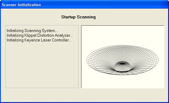
Initializing Klippel Analyzer hardware

The vibration measurements are conducted with the Distortion Analyzer or KLIPPEL Analyzer 3 device. During the initialization, a test vibration measurement is started to check the correct connection and working of the Analyzer hardware.

If no Analyzer hardware is connected or the current device has no proper measurement Licences, then a dialog will pop up asking for Available Devices.

If the power amplifier is not connected properly you will see an error message: No proper amplifier output.

Initializing Keyence Laser Controller

A serial connection between the operating PC and the Keyence Laser Controller is necessary to set and check the Laser settings. The controller is checked for known connected Laser Heads and the Laser Parameters are automatically adjusted.

Note

If no serial connection to the Laser Controller can be found, a Keyence Laser Controller Error will be displayed.

Manual programming of the laser controller is possible. Please see the hardware manual, section Sensor Handling -> Laser Sensors.

Supported Laser Controllers and their Heads for SCN

Keyence LK~G3001P

LK~G32

LK-G82

Keyence LK-G5001P

LK-H022

LK-H052

LK-H082 (flat scan only)

The Keyence Laser Controller can be equipped and used with two laser heads in parallel. Head 1 needs to be connected to the sensor at the SCN system, head 2 can be used for any other application. The dBLab installation comes with several laser setting templates. For operation of two laser heads at one Keyence controller, the following templates can be used:

5a	LK-H052 @ head 1 + LK-H022 @ head 2
5b	LK-H052 @ head 1 + LK-H082 @ head 2
5c	LK-H052 @ head 1 + LK-H152 @ head 2
6a	LK-H022 @ head 1 + LK-H082 @ head 2

Refer to the hardware manual, section Sensor Handling -> Laser Sensors for details on programming the Keyence controller.

Note

Software releases of Version 210 or earlier do not support two laser heads during SCN operation. The second head has to be disconnected during SCN measurement and needs to be reprogrammed to the previous settings afterwards.

Motor Control Calibration

To assure a correct positioning of the Scanner Hardware the Motor Control needs a calibration each time when it has been switched off or disconnected from the PC. The current calibration state of the Motor Control is indicated by a green LED.

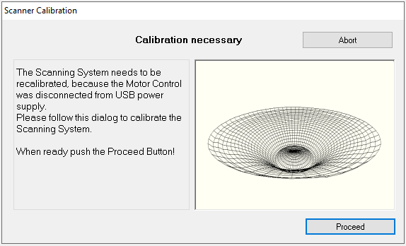
If a calibration is necessary, then a wizard dialog will be launched which guides quickly through the calibration steps.

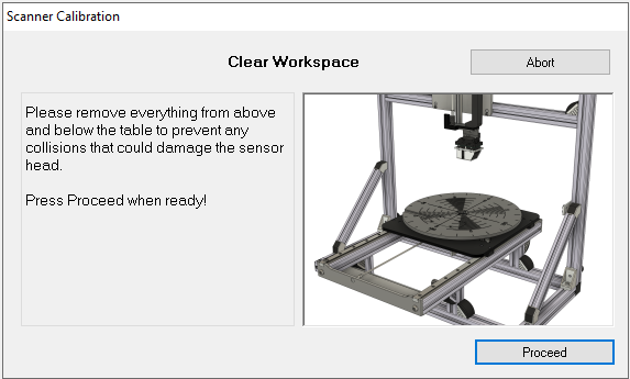
Please assure a safe operation of the scanner calibration. Any objects above and below the turntable are in danger of a collision with the calibrating laser.

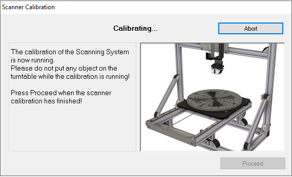
The Scanner Hardware is automatically driven into three end contacts: on the upper end of the Z axis, the rear end of the R axis and the counter-clockwise stop of the Phi axis. When the position of these end contacts is known to the Motor Control all following driving commands can be safely executed.

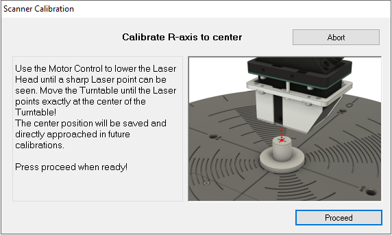
In a second calibration step the rest position of the Turntable below the Laser Head can be adjusted. The rest position of the R axis will be saved and directly approached after the next calibration.

If the Scanner Hardware has been reassembled or the Scanning Software has been reinstalled, the exact rest position of the turntable has to be readjusted. Refer to the section First Calibration for a step by step guide.

Important! A correct positioning of the Laser Head over the center of the Turntable is essential for measuring correct vibration and geometry data.

Scanning Procedure

This section describes the necessary steps to start a new vibration scanning task.

Start new Project

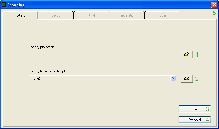
A new scan setup starts with the choice of a new Project File [1]. It is possible to choose an existing scanning project as Template [2] for the new scan. All setup parameters from the template will then be copied to the new scan setup.

If an existing project file is chosen to be overwritten, the existing setup will also be used as Template for the new scan.

You can always go back to the Start and Reset [3] the current scanning project.

Press Proceed [4] to specify the General Scan Setup

You can abort the scanning process by closing the Scanning Window [5].

General Scan Setup

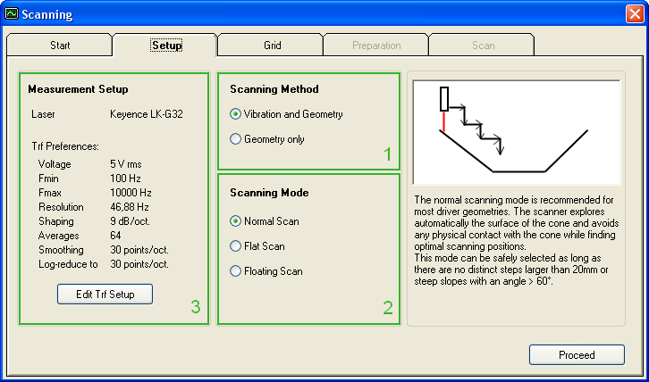
Two general Scanning Methods [1] can be selected, a complete Vibration and Geometry scan or a reduced scanning of the Geometry only.

In case a Geometry scan is selected, the TRF Preferences (3) of the Transfer Function measurement with the Analyzer hardware are automatically adapted for optimal scanning speed and geometry accuracy.

For a normal Vibration and Geometry scan the TRF Preferences (3) can be changed to adapt to the current driver. See also the description of the TRF Setup.

The Scanning Mode [2] influences the strategy of the automatic scanning process to explore the driver geometry in a quick and safe way.

A Normal Scan is recommended for most applications. The scanner explores automatically the surface of the cone and avoids any physical contact with the cone while finding optimal scanning positions. This mode can be safely selected as long as there are no distinct steps larger than 20mm or steep slopes with an angle > 60°.

For a Flat Scan the vertical position of the laser head will be fixed during the scan leading to a higher scanning speed and highest accuracy in the measured geometry. As only the focal range of the laser head can be used for the scanning, this mode is only recommended for very flat driver geometries like flat tweeters, headphone drivers or micro speakers.

During a Floating Scan the vertical position of the laser head will always stay above a minimal value. By limiting the minimal driving height it is possible to scan drivers below a transparent layer e.g. while measuring in vacuum. Also the robustness of the scanning is increased passing over steep gaps in the cone surface.

After specifying the General Scan Setup you can proceed to the setup of the Measurement Grid

TRF Setup

The TRF Measurement Setup defines the parameters for the vibration measurement at each grid point.

Frequency Settings

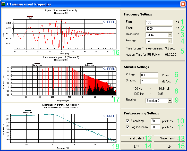
The frequency range for all TRF measurements will run from a lower frequency Fmin [1] to an upper frequency Fmax [2] in certain Resolution [3] steps.

Fmax can reach up to 25 kHz, but must of course be larger than Fmin. The Resolution steps are fixed and depend on the Analyzer Hardware and Fmax.

A certain number of Averages [4] can be selected for each measurement point to increase the signal-to-noise ratio.

The Frequency Resolution and the number of Averages have a large influence on the measurement time for the total scan. With the Estimated Scan Time [5] a rough hint is given, how long the actual scan will take.

Stimulus Settings

To measure the cone displacement with sufficient signal-to-noise ratio a shaped stimulus is used. The (rms) Voltage [6] of the shaped stimulus can be adapted to the currently measured loudspeaker.

The specified Voltage will be reached at the highest frequency Fmax, while all lower frequencies will be attenuated according to the Shaping [7].

For finding a proper Voltage setting it is strongly recommended to start with a very low voltage and to cautiously increase the voltage until the desired signal-to-noise ratio is reached.

A logarithmical Shaping [7] of the stimulus can be changed within a range from 0 dB(V) per octave up to 12 dB(V) per octave. Usually a shaping of more than 6 dB per octave should be applied to protect the loudspeaker from too high voltages and displacements. A summary of the Shaping Settings [8] is also given.

Warning

Caution! A too high voltage or a too low shaping can damage and destroy your loudspeaker! No warranty is given for any measured loudspeaker.

It is possible to change the signal Routing [9] for the Analyzer hardware to switch between Speaker Channel 1 and Speaker Channel 2.

Postprocessing Settings

An adjustable Smoothing [10] can be used to improve the measured transfer function. The default smoothing of 30 TRF lines per octave is a good compromise between resolution and accuracy of the result curves.

A second post-processing option is to reduce the resolution of the frequency axis in logarithmic scale. The Log-reduce [11] decreases the data volume to a certain number of lines per octave which can be set in the according text field. That option is very efficient to reduce the amount of collected scanning data and increase the speed of the analysis. It should be used in combination with enabled Smoothing [10].

Result Plots

Three result charts of the last conducted TRF measurement are shown. The Signal Y2 vs. time [16] shows the averaged time signal of the laser displacement.

The chart Spectrum of signal Y2 [17] shows the signal and noise spectrum of the laser signal. If the signal-to-noise ratio is too low in the desired frequency range, then try to increase the number of Averages [4] or increase the Voltage [6] and adapt the Shaping [7].

The chart Magnitude of transfer function H(f) [18] shows the displacement transfer function which will be finally saved for each measurement point during a vibration scan. The transfer function is displayed with the chosen Smoothing [9].

By pressing the Reset Defaults [12] button all changes in the TRF setup are discarded and the default measurement setup is loaded.

It is possible to export the last TRF operation into a Klippel database file by pressing the Save Results [13] button. The Klippel database can be opened with the Klippel dB-Lab software and contains the setup parameters and all results of the last TRF measurement. Multiple TRF operations can be saved into the same database file for comparison.

Please send this database file to support@klippel.de in case you encounter any problems with the TRF measurements.

See also the section Malfunction and Troubleshooting for solving problems with the TRF Measurements.

Measurement Grid

The Setup of the measurement grid defines number and positions of the vibration measurement points. Various options can be used to customize the scanning grid according to the respective loudspeaker and task.

Presets

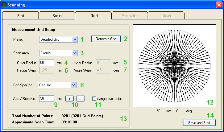
A certain grid Preset (1) can be selected to define a well-spaced measurement grid in a quick way.

The following Presets can be chosen:

Detailed Grid

Points: 3201

Comprehensive scan of the complete loudspeaker

Explore Grid

Points: 451

Overview scan to see the main vibration properties

Profile Grid

Points: 51

Quick scan of one radial profile line

Ring Grid

Points: 60

Quick scan of a ring at one radius

Sd Grid

Points: 451

Practical scan for calculating the effective radiation area S_D, see Effective Radiation Area SD

Manual Grid

Points: 1-50000

Grid adapted to the respective task

By clicking on the Generate Grid [2] button, the entered grid parameters are used to create a new measurement grid which will be shown then in the Grid Picture [12].

The total number of actual Measurement Points [13] will be lower for a Rectangular Scan Area [3] and for a Sparse Grid Spacing [8].

Scan Area

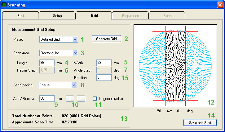
In addition to the grid preset, it is possible to select the type of the defined Scan Area [3].

For a Circular Scan Area the Outer Radius [4] of the loudspeaker can be specified, while for a Rectangular Scan Area the Length [4] and Width [5] of the driver can be changed.

If necessary also a Rotation Angle [15] can be specified for rectangular scans.

Grid Spacing

The Grid Spacing [8] allows more influence on the actual placement for the measurement points.

A Regular Grid Spacing will prescribe an equal distribution of measurement points for each radius and angle.

Using a Radial Irregular Grid Spacing increases the density of the scan radii in the outer cone region where a more intricate vibration behavior begins.

Another option is to apply a Sparse Grid Spacing where the measurement point density is reduced towards the center of the driver to save scanning time.

Manual Grid

If the Manual Grid Preset is chosen, then also the regular spacing of Radius Steps [6] and Angle Steps [7] can be adapted. For a Circular Scan Area [3], an Inner Radius [5] can be specified.

The distribution of the different scan radii can be further influenced by adding or removing single radii. For this the desired Radius [9] needs to be typed in and by using the Add / Remove Radius [10] buttons the manual grid can be changed.

The manual creation or removal of single radii will be reset when choosing a predefined Preset [1] or clicking again on the Generate Grid [2] button!

Dangerous Radius

For loudspeaker cones with high steps (>20mm) or deep gaps in the geometry it is necessary to avoid a collision of the laser head with the cone surface.

This can be accomplished by either limiting the Z driving position with a Flat Scan or Floating Scan mode, see General Scan Setup or by specifying a Dangerous Radius.

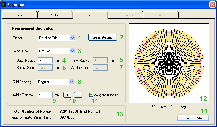
Specify a new dangerous Radius[9] by using the Dangerous Radius [11] check box.

In the Grid Picture [12] the Dangerous Radius will be marked as a red circle and the range of its influence will be marked with additional orange circles.

Within the influence range of one Dangerous Radius the laser head will only be positioned to a safe Z height. The safe Z height is derived from the highest point of the driver which has to be determined during the Scan Preparation steps.

The number of measurement points and an estimation of the probably required scan time is shown in the Scan Summary [13].

Start the Scan Preparation steps by clicking on the Save and Start [14] button.

Scan Preparation

The Scan Preparation steps are necessary to assure a correct and secure scanning procedure. Please follow the steps as shown below.

1. Place the driver on the turntable and connect the speaker cables

   

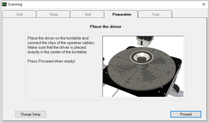
   You can always Change the Setup again by clicking on the respective button.

2. It is necessary to determine the highest loudspeaker point for a Normal Scan and a Floating Scan as specified in the General Scan Setup

   

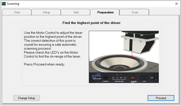
   This highest point will serve as reference position to assure a safe scanner movement passing over unknown cone geometry. It is furthermore reference for a safe driving distance above Dangerous Radii, if specified for the current Measurement Grid.

   You cannot pass by this step unless the laser signal is in the ok-range!

   At this point also the Laser Calibration is checked and can be renewed in case the laser is not properly calibrated.

3. For a Flat Scan the fixed driving height can be adjusted, which will be used for the complete scanning process.

   

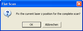
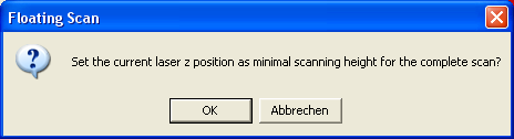
   Likewise for a Floating Scan the minimal driving height can be adjusted during the scan preparation.

   

4. After the first measurement point has been approached it is possible to check the correct position of the laser head above the loudspeaker a last time.

   

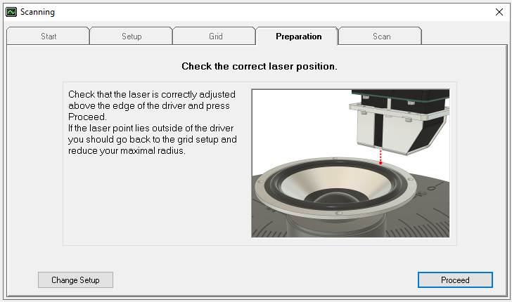
   Press Proceed to start the Scanning now.

Scanning

The Scanning Process runs automatically and does not need any interference from the user.

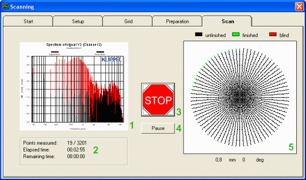
The current Laser Signal Spectrum [1] is shown for each measurement point.

A Summary [2] is given over the already Measured Points and the remaining Scan Time. The time estimation is based on the time which was needed for the already finished points.

In case the scanning process needs to be immediately interrupted, the Stop [3] button will abort all Motor driving commands and TRF measurements.

Alternatively, the Pause [4] button will also stop the scanning process, but the current measurement and Motor driving task is finished first.

Warning

Important! Use the Stop button if any Malfunction of the Scanner occurs!

The scanning process can be resumed after an interruption as long as the position of the loudspeaker has not changed.

In the Grid Picture [5] the current progress of the scanning can be observed.

When the scanning process has finished the results can be visualized, see section Review and Analyze Scans.

Direct Motor Control

The Direct Motor Control tool can operate the Motor Control device via software commands. The current state of the Motor Control is shown and driving commands can be executed.

A quick access to the tool is available by pressing the Hotkey F5.

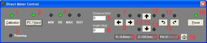
The Calibration [1] Led indicates the calibration state of the Motor Control. The calibration can be restarted by pressing the Calibration Button.

The PC / Hand LED [2] shows the current operation mode of the Motor Control. Pressing the PC / Hand Button Button toggles the operation mode and stops any currently running driving commands.

The Running LED [3] indicates whether the Motor Control is currently executing a driving command.

Warning

Important! No new driving commands can be executed while the Motor Control is running or locked by the scanning process! Only the PC / Hand Button [2] can still stop the currently running command.

The Laser State LEDs [4] show the current state of the Keyence Laser Head.

In the Distance [5] input field a certain value for the next driving command of the Z or R axis can be set. Likewise a value in the Angle [6] input field will be used for the next driving command for the Phi axis. The smallest possible driving Distance is 0.02 mm and the smallest turning Angle is 0.03°deg.

The R Axis LEDs [7] indicate an end contact of the R axis. Driving commands of the R axis can be started by the R Axis Buttons [8] below and the current Radial Location [9] of the hardware is displayed when the Motor Control is calibrated.

Likewise the Z Axis LEDs [10] indicate an end contact of the Z axis and new driving commands for the Z axis can be started by the Z axis Buttons [11]. The according Z-Position of the laser is shown in the Z-Display [14].

The Emergency Stop LED [12] will become red in case a normal end contact had failed and the scanner hardware touched an emergency contact. Please contact support@klippel.de in case an emergency stop has occurred!

To protect the Laser Head, the Laser Collision LED [13] can show a collision of the Laser Head if a Laser Collision Sensor is connected to the Motor Control. Detailed information about the hardware setup can be found in the section Setup of the Scanning System.

Finally the Phi Axis LEDs [15] show the end contacts of the turntable and new turning commands can be launched by the Phi Axis Buttons [16]. The current angle of the turntable is shown in the Phi-Display [17].

When the Motor Control is calibrated then the Home Button [18] can be used to approach the center of the turntable. The center position can only be changed during a new Motor Control Calibration.

The Power [19] button can be used to trigger a reconnect in case the Motor Control device has been switched off or the USB connection to the PC has been interrupted.

Hardware Check

The Scanner Hardware Check is a tool for troubleshooting errors of the Scanner Hardware and the Motor Control device. It can be accessed by the Klippel Scanning System menu entry Tools ‣ Hardware Check.

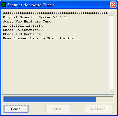
A new Hardware Test will be started by pressing the Run TesT button.

After the Hardware Test has finished, a detailed log file can be saved with the Save Log as… button.

A complete log file contains valuable information for analyzing errors by Klippel GmbH and should be attached to an email to support@klippel.de in case when errors have occurred in connection with the Motor Control device.

Laser Calibration

Before each scanning task the Laser Calibration is checked by comparing the laser signals before and after a motor movement of the Z axis of 1 mm. Therefore it is normally not necessary to perform a separate laser calibration before using the Scanning System.

In case the laser is not properly calibrated, a warning message appears that requests a new calibration.

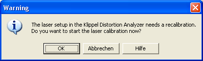
The scanning process can still be continued if this warning is canceled, but the vibration measurement results will be most likely incorrectly scaled!

Laser Calibration with KLIPPEL Analyzer 3

Using the SCN in combination with the KLIPPEL Analyzer 3 the calibration of the Laser is usually performed automatically by SCN Software.

Alternatively the Laser can be calibrated manually using the dB-Lab LC KA3 Laser Calibration module. Detailed descriptions are given in the hardware manual, see section Sensor Handling

Laser Calibration with Distortion Analyzer

The Laser Calibration tool can be used to calibrate the laser sensor for measurements with the Distortion Analyzer. The calibration can be started by the menu Tools ‣ Laser Calibration

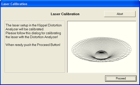
The Laser Calibration Dialog guides through the different calibration steps. Follow the indicated steps in the Klippel Distortion Analyzer menu until you reach the page where a defined calibration distance needs to be entered.

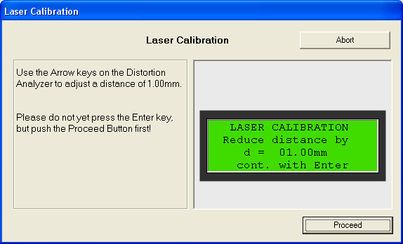
Adjust a distance of 1.00 mm in the Distortion Analyzer and press the Proceed button in the Laser Calibration Dialog. Now the laser head will be moved by exactly that specified distance of 1.00 mm by the Motor Control device.

Finish the laser calibration by properly exiting the Distortion Analyzer menu as indicated in the Laser Calibration Dialog steps.

Review and Analyze Scans

This chapter describes all functions of the Klippel Scanning System related to the review and analysis of previously measured scan data.

Animation

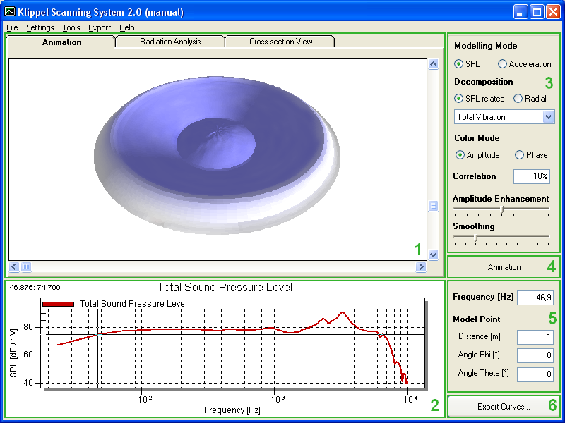
On the bottom of the screen there is a graph of the modeled sound pressure of the measured loudspeaker [2]. It is possible to select the currently displayed frequency by clicking on the graph.

Alternatively there are text input fields [5] to the right of the sound pressure graph. There you can also enter the current Frequency and specify the Model Point of the sound pressure modeling.

The three analysis tabs are each divided into a graphical representation on the left side [1] and a set of different Visualization Options [3] on the right side

The animation tab shows a 3D graph of the measured cone. By toggling the Animation [4] button you can start and stop the 3D animation.

The speed of the animation can be changed in the Settings menu by specifying the Period Time for one animation cycle. If the animation cannot be calculated in real-time then the actual animation cycle will be longer. To assure a fluent animation for this case the Save Movie File dialog can be used.

Two special mouse interactions are used to shift and zoom the 3D graphic object in the animation window. By pressing the Left Mouse Button and moving the mouse up and down while holding the button pressed you can Zoom the 3D view in and out. The same procedure with the Middle Mouse Button can be used to Shift the visual rest position height of the 3D object up and down.

A Right-Click on the 3D animation will show a Popup Menu where several Viewing Options can be selected to customize the visual appearance of the animation. The entry Reset View in the popup menu will reset the zoom and shift parameters of the 3D graphic to default values.

By using the Popup Menu it is also possible to display the current Frequency directly in the 3D animation. This is useful for including the frequency into exported pictures or movies.

The Export Button [6] saves all calculated curves in a .kdb file which can be opened and viewed by the dB-Lab software.

Radiation Analysis

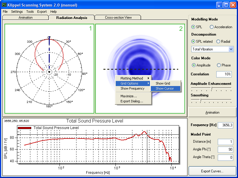
The Radiation Analysis tab can be used to investigate the modeled directivity of the radiated sound. The Visualization Options are identical to the options on the Animation tab.

On the left side a polar Directivity Plot [1] is showing the modeled sound pressure at several receiver points on a hemisphere over the center of the measured speaker.

The receiver points of the directivity modeling are placed along one specific angle Phi above the speaker surface which is indicated by a black dotted line in the Amplitude Distribution Plot [2] on the right side. The black line can be moved by a Left-Click on the amplitude distribution plot or by manually specifying a certain Angle Phi for the sound modeling receiver point on the bottom of the screen.

A special option in the Calculation Preferences menu can be selected in case rather an Averaged Directivity over several angles Phi above the speaker surface is preferred.

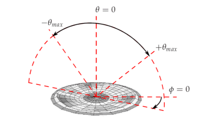
The modeled directivity is only valid (and displayed) for a maximal opening angle Theta = .

The Directivity Plot [1] is always displayed relatively to its maximum value.

The Amplitude Distribution Plot [2] is a compact illustration of the absolute vibration amplitude on the measured surface. In comparison to the 3D Animation it does not show the instantaneous excursion but the absolute vibration amplitude at all measurement points.

A grid and a data cursor can be switched on by the Popup Menu to determine the position of certain amplitude maxima or minima.

Cross-sectional Cut

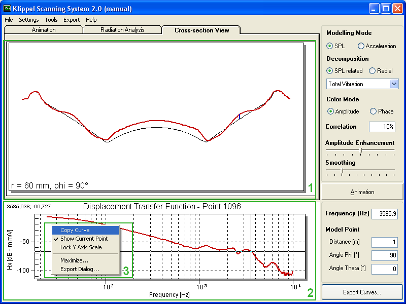
The third analysis tab shows an animation of a Cross-sectional Cut [1] through the measured speaker. The Visualization Options are identical to the options on the Animation tab.

Hereby the plot of the modeled sound pressure in the bottom is replaced by a plot of the measured Displacement Transfer Function [2] at the selected measurement point. If the modeled sound pressure shall be shown instead, then the option Show Current Point [3] in the Popup Menu can be deselected.

The radius of the measurement point can be chosen by clicking in the Cross-section Animation [1] window. A blue line indicates the position of the selected point. The angle of the selected cross-section is equal to the Angle Phi of the Model Point which can be chosen in the lower right corner of the screen or alternatively also in the Amplitude Distribution graph of the Radiation Analysis tab.

Interpolated points in the cross-section animation are marked with black spots if the option Mark Interpolated Points in the Settings menu is selected.

The currently selected point can be removed from analysis by right-click on the Cross-section Animation [1] and selecting the option Corrupted Point. That is an additional option to remove invalid measurement points when setting a higher Correlation threshold is not sufficient or applicable.

The curve data of the Displacement Transfer Function [2] can be copied to the clipboard using the Popup Menu entry Copy Curve [3]. This curve data can now be imported into any text editor and especially into the graphs of the Klippel dB-Lab software.

A better visual comparison of the displacement curves of different measurement points can be accomplished by Locking the Y-Axis scale [3] using the Popup Menu.

Sound Power

The prediction of the radiated Sound Power is a special feature which can be found via the menu item Tools. If there are previously calculated results available they will be shown instantly.

You will need a special licence from Klippel GmbH to be able to run a new Sound Power calculation!

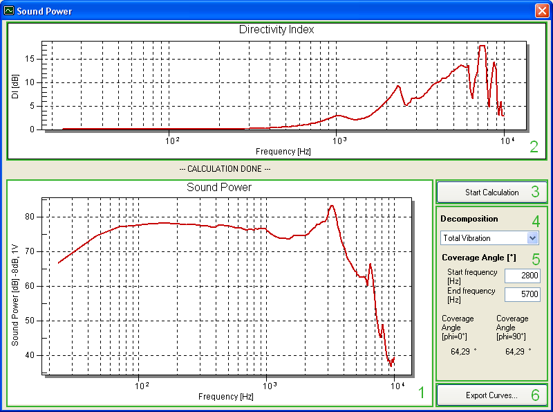
At the bottom of the window, the Sound Power Plot [1] shows the sound pressure integrated over a hemisphere.

In order to allow a direct comparison between the sound pressure level (SPL) and the sound power level, the sound power curve is adjusted based on the distance used for the sound pressure calculation.

\[L_{P,scaled} = L_P + 20 \cdot log10 \left( \sqrt{\frac{\rho_0 \cdot c \cdot P_0}{p_0^{2} \cdot 2 \pi } }\cdot \frac{1} {r}\right)\]

For instance, to align the SPL at a distance of \(r = 1 m\), the sound power level is reduced by about \(-8 dB\)

The Data Decomposition [4] technique can also be applied to the sound power response (total, radial, circular).

The continuous red line always shows the chosen component. If the radial or circular component is selected, the Total Sound Power is shown as a black dashed line.

At the top the Directivity Index Plot [2] shows a graph depending on frequency that is characterized by the ratio of the SPL on axis to the overall radiated SPL averaged in the half space. A Directivity Index of 0dB means that there is a radiation with equal intensity over the whole half space.

By pushing the Start Calculation Button [3] a new calculation begins if either no data is available or if any setting has changed (correlation, frequency limits for Coverage angle).

The Coverage Angle describes the directivity in a particular frequency range where the sound pressure level drops down -6dB from the maximum. The radiation property is evaluated for 2 orthogonal planes whereas the planes contain the reference axis. Therefore two single values for each plane will be yielded in a frequency range from 2800Hz to 5700 Hz by default as defined in the IEC standard 60268-5. Regarding the effective frequency range the limiting frequencies can be adjusted near the upper limit of the effective frequency range with a Start and End frequency [5].

The Coverage Angle has a resolution of 11.25 due to the limited resolution of the half space mesh.

Effective Radiation Area SD

The calculation of the Effective Radiation Area SD on base of the scanning results can be accessed in the menu Tools ‣ SD Calculation.

You will need a special licence from Klippel GmbH for the SD calculation!

On the upper left side the Cross-sectional Cut [1] of the measured loudspeaker is shown at a given angle. Blue markings visualize the selected averaging radius on each side of the loudspeaker.

At the top right the Amplitude Distribution Plot [2] is shown with a dashed line referring to the Cross-sectional Cut [1] and a red circle indicating the selected averaging radius. The angle of the cross section can be selected by clicking on the picture [2].

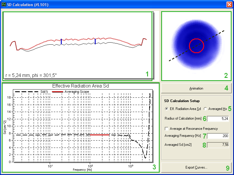
The shown Amplitude Distribution and vibration behavior in the Cross-sectional Cut always refers to the frequency in the main window!

On the bottom of the window the graph of the Effective Radiation Area Sd [3] depending on frequency is displayed. The red range shows the scope of frequency averaging which leads to a single value for SD [8].

The Animation Button [4] shows the vibrating diaphragm of the scan at a pre-selected frequency and modeling mode. Therefore it can give advice about the position of the voice coil and the most appropriate placing for the averaging radius.

Check boxes for the effective radiation area and the averaged displacement transfer function Hx [5] enable the switching between those curves which are shown in the bottom chart [3].

The Averaging Radius [6] can be entered or changed by clicking on the Cross sectional Cut [1]. Selecting an averaging radius within the voice coil provides a very stable value for S_D.

When the checkbox Average at Resonance Frequency[7] is selected, than the effective radiation area will be determined by averaging around the resonance frequency. Otherwise the Averaging Frequency [7] can be chosen manually.

The final value for the Effective Radiation Area SD [8] is averaged in a frequency range from 0.5 up to 1.5 the Averaging Frequency [7].

Preferably the graph S_D(f) has a wide plateau in which the single value for S_D should be read. The frequency range of averaging is marked by a red line. A text message is shown if the selected Averaging frequency is presumably too high or too low.

If a certain averaging radius does not contain valid measurement data an error message will be shown. Also if the SD-value exceeds the total scanned area a warning message will be shown.

The Export Button [9] saves the curves for the effective radiation area, the displacement and its phase in a .kdb file which can be read by Klippel dB-Lab. There the figures for the averaging scope, resonance frequency, averaging radius and averaging points are listed in a table.

Visualization Options

The visualization options apply equally for all three graphical representations.

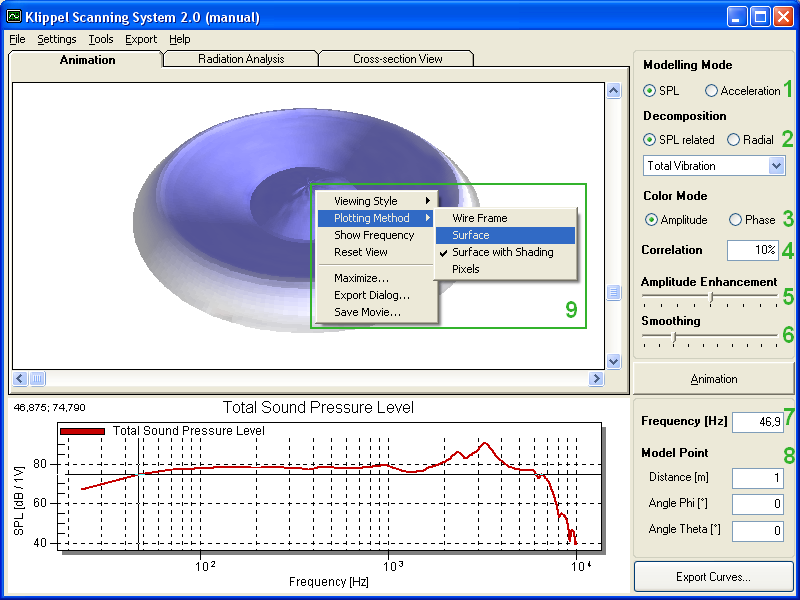
Modelling Mode

Two different Modelling Modes (1) can be used to analyze the total behavior of the loudspeaker, the SPL and the Acceleration Mode.

The SPL Modelling predicts the radiated sound pressure level of the measured cone surface based on a simple Rayleigh integral model. That means the sound pressure at the Model Point is predicted by a summation of point sources placed at each measured point on the cone.

The Acceleration Modelling shows instead a summation of the absolute acceleration on the cone, without considering the vibration phase. It is scaled in accordance to the sound pressure from the SPL Modelling to allow a direct comparison of surface motion and resulting sound radiation.

Data Decomposition

The Data Decomposition [2] can be used to separate single vibration components with specific information. Two different decomposition schemes can be selected, a decomposition into radial and circumferential vibrations and a second decomposition in relation to the modeled sound pressure at the receiver position.

The selection of a certain vibration component affects all post-processing operations. That means the graphical representations and the modeled sound pressure are only showing the contribution of the actual vibration component.

The Total Vibration shows the complete surface vibration as measured with the laser scanner.

Radial / Circular Decomposition

The Radial / Circular decomposition is solely based on the measured cone vibration. The Radial Component averages the vibration along each radius and simplifies the vibration picture. The radial membrane motions are mainly responsible for the sound radiation in axis.

By subtracting the Radial Component from the Total Vibration the remaining Circumferential Component is determined. It comprises all vibrations which deviate from the mean vibration along each radius. Any asymmetric cone movement can be revealed by looking at the Circumferential Component.

The radial/circular decomposition is only valid for axis-symmetrical loudspeaker scans and requires a proper centering of the speaker on the turntable!

SPL Related Decomposition

For the SPL related decomposition the modeled sound pressure at the Model Point is used to separate three special vibration components. The In-Phase Component shows the vibration which is exactly aligned with the total sound pressure. It shows all motion which is responsible for the sound radiation to the receiver point at the selected frequency.

The Anti-Phase Component is the counterpart of the In-Phase Component because it comprises the motion which relates to the produced sound pressure with a 180° phase shift. That means the Anti-Phase Component effectively reduces the radiated sound to the receiver point.

Finally, the Quadrature Component is orthogonal to the radiated sound pressure. Its vibration does neither increase nor reduce the sound pressure at the receiver point. Looking only at the Quadrature Component the contribution to the sound radiation of all points will sum up to zero.

Color Mode

Two different methods of coloring the visualization data can be chosen [3]. By selecting the color mode Amplitude the color of the 3D surface represents the instantaneous displacement amplitude with a blue color tone for positive displacement and a red color tone for negative displacement. The intensity of the color is relatively scaled proportional to the amplitude.

The Phase coloration is instead showing the instantaneous displacement phase of the 3D surface. The colors red and yellow represent a phase difference of 180° degree.

If the Viewing Style of the 3D animation is set to monochrome, then both coloration schemes are adapted. Then the amplitude coloration will show a high instantaneous displacement amplitude with a dark color, a separation of positive and negative displacement is not possible anymore. On the other hand the phase coloration can still show phase differences of 180° degree between regions with the colors black and white.

Correlation

To verify the quality of each laser measurement point a correlation parameter between two separate measurements at the same point is determined. A correlation of 100% means that two measurements at the same point gave exactly the same vibration data, while a correlation of 0% means that the two measurements gave completely different results.

The correlation is an important tool to remove bad measurement points from the visualization and analysis.

The specified Correlation [4] parameter sets a threshold for the minimal required correlation of a measurement point to be visualized and included in the analysis.

All points with a correlation value lower than this threshold will be interpolated in the graphical representations and excluded from the sound pressure modeling.

If the Correlation is set to 0% then all measured points are shown and used for the sound pressure modeling.

A special option in the Settings menu can be selected to highlight all interpolated points with a gray color.

Another option to remove bad measurement points is to mark them as Corrupted by right click on the respective point in the Cross-sectional Cut

Amplitude Enhancement

The vibration amplitude is scaled relatively to the mean amplitude in the respective chosen view to supply a good picture of the surface motion. The Amplitude Enhancement [5] slider can be used to manually scale the visualized amplitude higher or lower than the standard scaling.

The amplitude scale is logarithmically spaced to provide an additional scaling from –20dB to +20dB in relation to an automatically determined standard scaling at 0dB.

Although the scaling is determined relatively to the actual vibration amplitude of the measured motion, the scaling will be fixed among the different vibration components belonging to one vibration decomposition set.

Note

Please note that the vibration amplitude will be clipped in the visual representation if it supersedes a certain maximal value!

Smoothing

To remove measurement noise a visual smoothing of the measurement data can be done. Hereby a spatial Gaussian smoothing filter is applied to the vibration data and the power of the smoothing can be adjusted with the Smoothing [6] slider.

If the slider is moved to the left most side then no smoothing is applied to the data. The higher the smoothing value is chosen the larger is the influence of the smoothing filter.

Only the vibration data is smoothed, the geometry data remains unchanged.

The smoothing affects only the graphical representations but not the sound pressure modeling!

Frequency

The current analysis Frequency [7] for the scanning results can be either changed by typing into the respective input field or by clicking with the Left Mouse Button into the Sound Pressure Plot at the bottom.

Model Point

All Sound Pressure modeling calculations are only valid for a certain Model Point [8].

The coordinates of the Model Point [8] are given in a polar description by a certain Distance from the center of the measured cone surface, an Angle Phi describing the angle in plane with the cone surface and an Angle Theta orthogonal to the cone surface.

The Angle Phi corresponds to the angular scale as indicated on the Scanner Turntable.

An Angle Theta of 0 degree describes a Model Point exactly on axis. A point outside of the maximal opening Angle Theta = cannot give reliable Sound Pressure Modeling results and is excluded from the analysis.

Popup Menu

Some visualization options can be accessed by a Popup menu [9] which appears on a Right Click with the mouse on the respective graphical representation.

The Popup Menu content is specific for each picture. A complete list of all possible mouse interactions and popup menus can be found in the section User Interactions.

Settings

The application settings can be accessed by the menu entry Settings ‣ Preferences. Three tabs are shown there, first the Animation Preferences, second the Calculation Preferences and finally the General Preferences.

A quick access to the Preferences is possible by the Hotkey F2

Animation Preferences

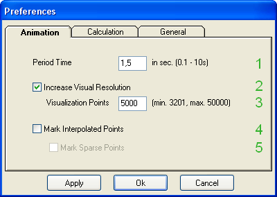
The Animation Preferences apply for all loaded scanning projects.

The Period Time [1] specifies the time for one animation cycle. The animation speed cannot be accomplished if the data processing effort is too high.

If the option Increase Visual Resolution [2] is selected, then the specified number of maximal Visualization Points [3] will be used to create a finer mesh resolution by interpolation from the measurement data.

A specification of a smaller number of points than the minimal number will have no effect. The maximal valid number of points is set to 50000.

With the option Mark Interpolated Points [4] it can be specified whether the interpolated points should be specially highlighted in the graphical representations.

It is useful to select this option to get a good imagination of how many points are really measured and how many points are only interpolated. For preparing an animation movie of a specific vibration motion it is possible to deselect this option and display the interpolated colors instead.

The option Mark Sparse Points [5] affects only the visualization of scans which have been measured with sparse grid spacing. If the option is checked, then the interpolated grid points from sparse point placement are also highlighted together with regularly interpolated points.

Calculation Preferences

The Reference Voltage [1] for all modeled sound pressure charts can be adjusted in the Calculation Preferences. The curves will be shifted according to the reference voltage to allow a direct comparison with external data.

A reference voltage of 2.83V is equal to an input Power of 1W for a driver with a nominal impedance of 8Ohm.

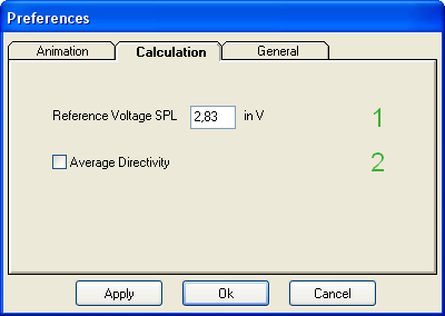
The option Average Directivity [2] applies for the Directivity plot in the Radiation Analysis tab. If it is selected then a number of different radiation angles are averaged for producing the polar directivity graph.

General Preferences

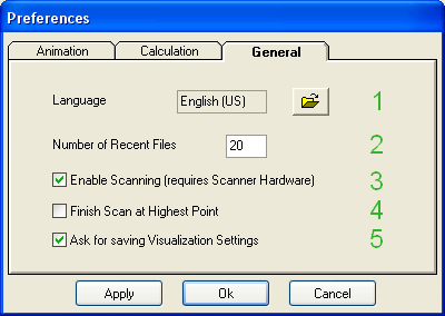
The General Preferences affect the complete Klippel Scanning System application.

To load a new Language [1] file please use the Open button and select a valid language file.

It is also possible to change the number of menu entries for Recent Files [2] within the range from one file to 20 files.

The Checkbox Enable Scanning [3] has to be selected to enable the control over the Scanner Hardware.

Please note, that only one instance of the Klippel Scanning System application can control the Scanner Hardware. But it is possible to compare several scans in different application instances at the same time.

If the Checkbox Finish Scan at Highest Point [4] is selected, then the Scanner hardware will approach the specified highest point of the current scan when the measurement has finished. That helps to speed up multiple scans of the same driver because the Scan Preparation steps can directly proceed without need to search again for the highest point.

The Checkbox Ask for saving visualization settings [5] can be used to reactivate the dialog which appears on closing a scan file.

When the Checkbox Remember Selection has been checked once, then that dialog will not appear anymore but the chosen option (Yes or No) will be applied for all scans.

Export Functions

The Klippel Scanning System provides a variety of export functions to make the results and graphical representations of the scan data accessible to external applications.

• A special Export Dialog is available in the Popup Menu of the graphical objects to provide access to a picture export to the Clipboard or to a File.

• The Export Geometry function provides a high precision geometry export into a common 3D CAD file format.

• It is also possible to export the complete set of measurement data to a text based file format by using the Export ASCII.

• The curve data of the Sound Pressure Modeling can be exported to the Clipboard via the Copy Curve entry in the Popup Menu.

• A more comfortable way to access the Result Curves is to export all sound pressure modelling curves at once to a Klippel database file and open them with the Klippel dB-Lab. You can do this via the Popup Menu entry Export Curves to Database.

• It is also possible to export a complete movie of the 3D Cone Animation or the Cross-sectional Cut via the Popup Menu entry Save Movie File.

Some Export Functions require a special licence for Additional Features

Export Dialog

All graphical components have access to the Export Dialog.

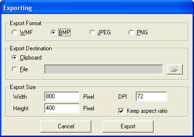
Export Format

WMF

The MetaFile format is a good method to export the objects image. The metafile will be able to adapt to varying output resolutions.

BMP

The Bitmap format is the most common image export format, however, it uses a large amount of memory.

JPEG

Similar to the Bitmap format, the JPEG format is compressed to take less memory. This format is widely used on web pages. This format is best suited for photographs because line art will be fuzzy due to compression. A better format for artificial graphics is the PNG.

PNG

Similar to the Bitmap format, the PNG format is compressed to take less memory. This format is gaining use on web pages and is most similar to the GIF format. This format will produce the best looking compressed raster images.

Export Destination

The Clipboard will be the most common destination. It provides a quick method of sharing information with other Windows applications.

When exporting to a File, the user has to supply a filename.

Export Size

The Export Size section changes depending on the selected Export Format.

The Metafile format is specified in millimeter units, while the other picture formats are given in Pixel units. The DPI input can be used to change the resolution of the pictures.

The default Export Size is set according to the current picture size in the Klippel Scanning System.

It is recommended to keep the aspect ratio of the exported picture locked to avoid unnatural stretching of the picture.

Export Geometry

The geometry of the measured loudspeaker cone can be exported by the menu entry Export -–> Export Geometry…

You will need a special licence from Klippel GmbH to be able to export the geometry data.

The geometry export will produce a 3D DXF file (AutoCAD R12 drawing exchange format).

Three different DXF export options are supported:

1. 3D Faces: All points are connected to a mesh to reproduce the surface of the measured cone.

2. Lines: The surface of the cone is given by single lines connecting the measured points

3. Points: Only the measured points are included in the DXF export

The exported geometry file can be opened with any software which supports the DXF file format. An example freeware DXF viewer is included in the scanning system installation and can be found in the installation folder \Toolsdxfviewer.

The geometry export files are defining all dimensional measures in meters using SI units.

Furthermore there is an export to STL file format possible, which is supported by various CAD tools.

Export ASCII

By the menu entry File –-> Export ASCII… it is possible to export a text file containing the complete set of measured vibration data.

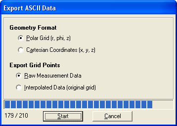
You will need a special licence from Klippel to be able to export the data.

Two different specifications of the coordinates of the measurement points can be used. The PolarGrid format will export the points in a polar coordinate system as it is natural to the scanning grid. It is also possible to convert the grid points to Cartesian Coordinates prior to the export.

It is recommended to export the Interpolated Data as shown in all animations and diagrams. That will fill up missing and corrupted points in the measured grid and also considers the currently applied Correlation threshold, but it will take more time to process the data for all frequencies.

Exporting the Raw Measurement Data will give the originally measured curves without any interpolation or detection of corrupted points.

By clicking on the Start button a dialog for saving the file will appear:

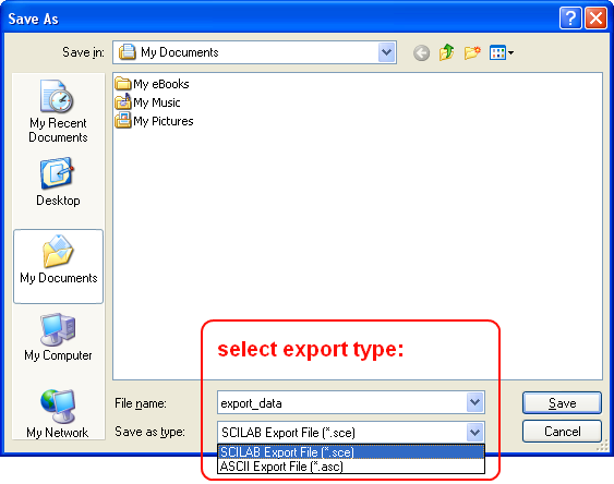
Two different file types for export are available:

ASCII Export File (*.asc) The data is exported in plain text format

SCILAB Export File (*.sce) The data is exported to plain text format, which can be interpreted by SCILAB. That allows an easier integration with different external programs.

It is possible to Import SCILAB Data again for visualization

Import SCILAB Data

External visualization data can be opened for visualization and analysis by using a text based import file which is processable by SCILAB.

Especially, previously exported scan data can be re-imported again for analysis after arbitrary processing steps performed with SCILAB.

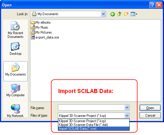
By the menu entry File -–> Open Scan… it is possible to select the file type Import SCILAB Data (*.sce) and import the data contained in that file.

A special licence is required for importing SCILAB Data.

Copy Curve

You can copy curves from the Sound Pressure Modeling chart and the Directivity chart and paste them into an arbitrary chart of a dB-Lab operation to compare different curves.

You can open the dB-Lab by choosing the menu entry Tools ‣ Run DB-Lab or by pressing the Hotkey F4.

To copy a curve, right-click on the chart and choose Copy Curve from the Popup Menu. To paste a curve in another dB-Lab window, right-click on the target window, and choose Paste Curve from the popup menu.

When a curve is copied to the clipboard, it uses a SCILAB-compatible format.

Export Curves to Database

All calculated curves of the sound pressure and acceleration modelling can be exported to a Klippel database file and analyzed further with the help of the dB-Lab.

That offers a quick way to compare the different curves directly and to investigate differences between surface acceleration and actually radiated sound pressure.

The calculated Sound Power curves will be also exported if available.

Save Movie File

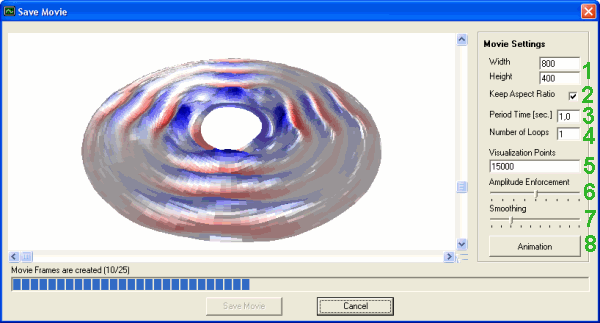
The movie export is a special feature which gives the possibility to save a certain animation in an “.avi” movie file. Several visualization options can be specified separately for the movie export.

The Width and Height (1) of the final animation movie can be chosen between minimal values of 72 Pixel and maximally 1224 Pixel.

It is possible to Keep the Aspect Ratio (2) of the movie locked.

The Period Time (3) of the final movie can be chosen to get the desired animation speed and resolution.

It is possible to create movie files with several animation Loops (4) after each other.

As the movie file does not have to be created in real-time, also a higher number of interpolated Visualization Points (5) can lead to a fluent animation.

The parameters Amplitude Enforcement (6) and Smoothing (7) can also be chosen separately for the movie file creation.

A preview of the movie can be watched by toggling the Animation (8) button.

By pressing the Save Movie button, the movie file creation will be started. At first the filename of the final movie file has to be chosen. Then all necessary movie frames are created.

Finally the movie file can be compressed by selecting an available video codec. A recommended video codec is the Cinepak Codec by Radius. Please wait until the movie file creation has been finished.

When the movie export has been successfully finished, the movie file will be opened with the standard movie player.

Scan Info

The Scan Info dialog gives a summary over the main measurement properties of the actually loaded Klippel Scanning Project file.

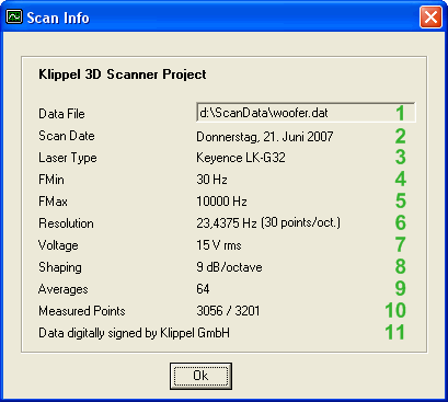
The following properties are shown:

Data File [1]

Scan data file associated to the project file

Scan Date [2]

Date of the scanning measurement

Laser Type [3]

Name of the Scanning Laser

Fmin [4]

Lower frequency limit for the Trf

Fmax [5]

Upper frequency limit for the Trf

Resolution [6]

Frequency resolution for the TRF (and log-reduction)

Voltage [7]

Applied TRF stimulus voltage

Shaping [8]

Applied TRF stimulus shaping for the Trf

Averages [9]

Number of TRF averages

Measured Points [10]

Number of successfully measured Points

Comment [11]

Comment for free Data signed by Klippel GmbH

A quick access to the Scan Info is possible by the Hotkey F3

User Interactions

Modeled sound pressure graph

Left mouse button	Click on graph to select current frequency
Right mouse button	show context menu: copy curve, lock y axis, maximize, export
←, →, PgUp, PgDown	Change current frequency
↑, ↓	Change cursor focus between graphs
E	Launch export dialog
M	Maximize

3D animation graph

Left mouse button	Drag up and down to zoom view
Middle mouse button	Drag up and down to move animation rest position
Right mouse button
←, →	Rotate view left, right
↑, ↓, PgUp, PgDown	Rotate view up, down
Ctrl + (↑, ↓, PgUp, PgDown)	Move animation rest position up, down
Alt + (↑, ↓, PgUp, PgDown)	Zoom in, out
Space Bar	Start Animation
E	Launch export dialog
M	Maximize 3D picture
R	Reset zoom and movement of the 3D picture
S	Switch viewing style (color / black and white)

Directivity graph

Left mouse button	Click on graph to select current angle theta of the receiver point for the sound pressure modeling
Right mouse button	show context menu: copy curve, maximize, export

2D amplitude distribution graph

Left mouse button	Click on graph or drag to select current angle phi for defining a cross-sectional cut through the speaker. This angle is also used for the receiver point of the sound pressure modeling
Right mouse button

Cross-section animation graph

Left mouse button	Click on graph to select one specific scan point (if show current point is enabled). The displacement transfer function at this point will be displayed on the bottom instead of the modeled sound pressure.
Right mouse button
←, →	Change selected radius (if show current point is enabled)
Space Bar	Start Animation
E	Export dialog
M	Maximize

Supported Modules for Im/Export

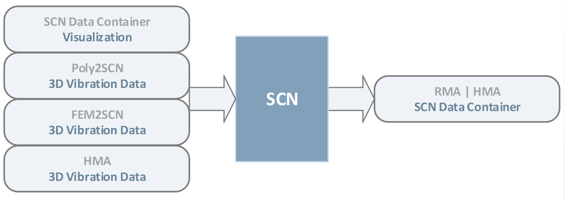
Motor Control Manual

The Motor Control device controls the Scanner Hardware by operating the three stepper motors and supervising all collision contacts as well as the laser signal range.

Warning

Never connect or disconnect a motor cable while a motor is running, the stepper motor drivers can be damaged!

Connect the Motor Control only to the dedicated Klippel hardware, other devices can be damaged! The Klippel GmbH assumes no liability to damages on other hardware than listed in the Connection Guide.

Front view of the Motor Control

Calibration Button

The Calibration Button (1) starts the Calibration, but it is only active in Manual-mode. During Calibration the Motor Control switches to PC-mode. The Calibration Led is green when the Motor Control is calibrated properly.

The Calibration performs the following steps:

1. Move Laser to upper Z-Axis End Contact

2. Move Laser back to the height, where the Calibration had started

3. Move Turntable to the rear R-Axis End Contact

4. Move Turntable away from the End Contact

5. Move Turntable to the counter-clockwise Phi-Axis End Contact

6. Move Turntable away from the End Contact and to the start position

Do not put a loudspeaker on the turntable, before the Calibration has finished!

The Motor Control needs a calibration after every Power switch-off or USB-lost.

Laser Signal Range

The four Laser Signal Range LED’s (2) indicate the clearance between the Laser head and the surface of the DUT.

If MIN, OK or MAX LED is lighting then the Laser is can measure the surface of the DUT. The OUT LED indicates that the Laser cannot detect the DUT surface. The Laser could be either too close or too far from the surface of the DUT or the reflected light has a too low intensity.

Use some kind of surface coating in case the DUT surface is (semi-) transparent and does not produce sufficient diffuse light reflections.

PC – Manual – Stop Button

The PC – Manual – Stop Button (3) switches between the two operation modes. PC-mode is activated for operating the Scanner Hardware from a PC during the Scanning. The Manual-mode has to be activated to control the Scanning Hardware directly from the Motor Control device.

To stop any PC operated scanner movement push the PC – Manual – Stop button and switch in Manual-mode. The last software instruction will be cleared. The PC - Manual LED is green in PC-mode and red in Manual-mode.

Driving Buttons

The six Driving Buttons (4) allow the manual positioning of Scanner Hardware in the three axes, each in two directions. These buttons are only active in Manual-mode.

Each axis has End Contacts at both ends. The End Contact LED’s indicate that an End Contact has been reached. In case of any End Contact only the complementary direction in the axis of the End Contact can be operated.

The manual driving up and down will stop, if the laser signal has reached the ok range.

If both End Contacts of one axis are lighting at the same time, then check the connections of the cables between Motor Control and Scanner Hardware.

Laser Collision LED

The Laser Collision LED [5] indicates that the Laser Collision Sensor has detected a collision. In case of a collision only a movement of the Z-axis in upwards direction is allowed.

The Laser Collision LED is also switched on when the Laser Collision Sensor is not connected properly!

Emergency LED

The Emergency LED [6] indicates a serious Scanner Hardware error. A normal End Contact has failed to occur and an Emergency End Contact was reached.

Please contact support@klippel.de in case an emergency stop has occurred!

Power Supply

The Motor Control needs the provided Power Supply [7] for the 24V DC voltage for the stepper motor drivers and the USB connection to supply the logic of the Motor Control.

For stand-alone operation without USB connection to a PC, an USB power supply would be necessary (e.g. a powered USB Hub).

The Power LED indicates the power state of the Motor Control. If the Power is switched on but the Power LED is off then check the USB-Supply-LED on the back of the Motor Control. If the USB-LED is off, then check USB-supply, otherwise check the 24VDC-supply!

Power down up cycles under 2 seconds can cause faults!

Malfunction and Troubleshooting

Overview

This section gives step-by-step instructions to localize errors and suggests remedies for problems with Licences, with the Motor Control device, with the SCN Hardware and with TRF Measurements.

Also a description of certain Error Messages from the Klippel Scanning System can be found here.

Licences

There are appropriate software licences from Klippel required for Viewing Scans, Performing Scans and for some Additional Features.

Klippel Licences are always bound to a certain KLIPPEL Analyzer Hardware device or an USB Dongle. If no appropriate device can be detected, then a dialog will appear asking for connecting a device with a properly installed licence.

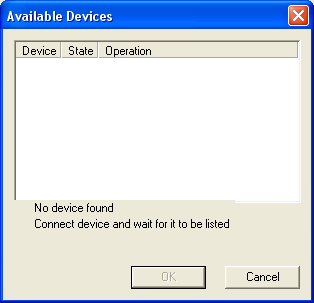
Please make sure that a Klippel Device is connected and switched on, for which appropriate licence files are installed.

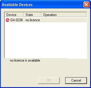
If no appropriate licences are found you need to Install new licence files for the associated dB-Lab installation

Install new licence files

Please contact support in order to request new licence files.

1. Start the associated dB-lab using the menu entry Tools ‣ Run dB-Lab in the Klippel Scanning System.

2. Select the menu entry Help ‣ Install Licence Files in the dB-Lab application.

3. Select the new licence files and install them.

If you get the licence files from Klippel as .klpack file, then it is sufficient to double-click on that file and install the licences via the upcoming dialog.

Viewing Scans

To view scan data it is necessary to have the required Klippel licence files installed. For viewing scans, which were digitally signed by Klippel GmbH no licences are needed.

Some Additional Features for the scanning data analysis can be licenced separately.

Performing Scans

For performing vibration measurements a valid licence for the Klippel TRF Module is required.

Furthermore since software release 2.0 there is a licence required for accessing the Scanner Hardware.

Please contact klippel@klippel.de in order to request new licence files.

Additional Features

These additional features need a separate licence:

Interface for FEA / BEA

Export of measured geometry and vibration data in various formats. Also necessary for importing external data files. See Export Geometry, Export ASCII and Import SCILAB Data.

Radiation Area SD

Calculate the effective radiation area from the scanned data, see Effective Radiation Area SD.

Sound Power / Directivity

Predict the radiated Sound Power.

Motor Control

Use the following checklist to solve problems with the Motor Control device and the Scanner Hardware:

1. Start the Direct Motor Control from the Tools menu in the Klippel Scanning System application.

2. Connect the Klippel Motor Control to the PC via USB and switch it on. Then press the Power button of the Direct Motor Control dialog.

   

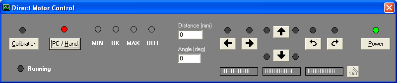   Motor Control after having been switched on, ready to run
3. Connect the Klippel Motor Control properly to the Scanner Hardware, see section Setup of the Scanning System. No Motor Control Error should be shown, otherwise check the cables.

   

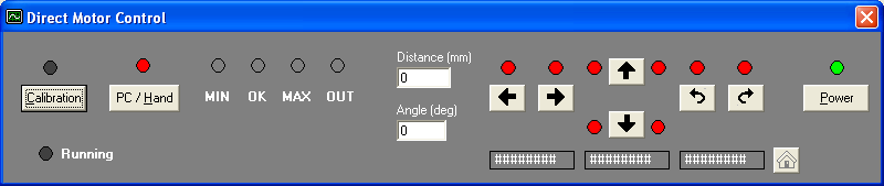   Motor Control indicating a Motor Control Error
4. In case a Scanner End Contact is indicated, drive the respective Motor away from the end contact by using the Buttons on the Motor Control device.

   

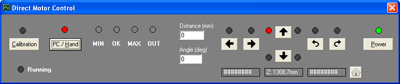   Scanner Hardware touching the Z up end contact
5. Calibrate the Scanner Hardware. Use either the Motor Control Calibration dialog or press the Calibration Switch on the Motor Control device.

   

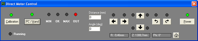   Scanner Hardware properly calibrated, the calibration Led glows

6. If the steps above could not be conducted successfully, run the Hardware Check from the Tools menu of the Klippel Scanning System and send the log file to support@klippel.de.

Refer also to the Motor Control Manual.

Diagnostics for the Motor Control USB and 24V_DC supply are described there.

SCN Hardware

Use the following checklist to solve SCN Hardware problems:

1. Z- or R-axis produces squeaking noises during movement.

   • Use some oil to lubricate the shaft. (Any light Oil for keys, bicycle chains and so on can be used.)

   • Drive the axis to one end point and loose the clamping nuts at the side that close to the motor. Fix the nuts without friction on the spindle. Drive the axis to the other end point and repeat the readjustment.

   • Plastic or rubber washer can be used to damp the vibrations of the spindle.

   • The spindle must be mounted without friction. (A small tension is better than pressure!)

2. Phi-axis motor is running but turntable is not moving.

   • Please contact support@klippel.de to get a detailed instruction to check for possible reasons.

   • If it is not only the loosened fitting of Phi axis gear box to the turntable a service at Klippel could be required. The turntable with Phi- and R-axis can be send in separately.

3. Motor drives with interruptions. Stuttering noise can be heard.

   • Check this behavior at another USB-port or PC. A bad USB ground connection could cause the Motor Control to this behavior. (Remove the USB hub, exchange the USB hub, use a powered USB hub or check for other possible impacting USB devices.)

   • Run the Hardware Check and send the log file to support@klippel.de. The Hardware Check is a tool for troubleshooting errors of the Scanner Hardware and the Motor Control device. It can be accessed by the Klippel Scanning System menu entry Tools ‣ Hardware Check Hardware Check.

4. One or more end contact LEDs lighting although all axis are away from end contact.

   • Both end contact LEDs of one axis are an indicator for a problem with the related connection. Check the connection, remove and plug the cable again.

   • Only one end contact LED is an indicator for a problem with one wire of the cable or the related switch at the SCN hardware. Exchange the related cable to check for broken wires inside. The Z-axis cable is a standardized RJ45 network CAT 5 cable. The R- and Phi-axis cable is a standardized D-sub 25 cable also used on PC parallel ports. Also the switches can be checked. Have a look below the cover of the Z-axis and below the turntable and press the switches manually. Check the related end contact LEDs at the Motor Control.

   • Collect your results and send this information to support@klippel.de for further help.

5. One axis is moving in the wrong direction.

   • The used stepper motors have a four wire interface. If one wire is missing the motor can also drive but with reduced force and random direction. Cables and connections have to be checked.

For support request to the Klippel customer service, please collect as much helpful information as possible:

• Save screenshots of error messages

• Save the log file from the hardware check

• Make some photos or video clips to point the problem

TRF Measurements

Use the following checklist to solve TRF measurement problems:

1. Connect the Analyzer hardware to the PC via USB and turn it on.

2. Make sure that a valid TRF Module Licence for this Analyzer hardware is installed, see section Licences.

3. Connect a Power Amplifier to the Analyzer hardware and switch it on, see section Setup of the Scanning System.

4. Connect a sample Loudspeaker to the Speaker Clamps on the Turntable and connect the Scanner Speaker Output to the Analyzer hardware, see section Setup of the Scanning System.

5. Connect the Keyence Laser Controller to the Laser Input of the Analyzer hardware and check the power supply of the Laser Controller, see section Setup of the Scanning System.

6. Check the connection between the Keyence Laser Head and the Keyence Laser Controller. If no red laser beam is visible, then reset the Laser Controller by disconnecting it from the power supply.

7. Connect the Keyence Laser Controller to the PC using a serial cable.

8. Assure that the Klippel Motor Control is ready to run, see section Motor Control.

9. Check that the Laser Signal shown at the Motor Control is in Ok range:

   

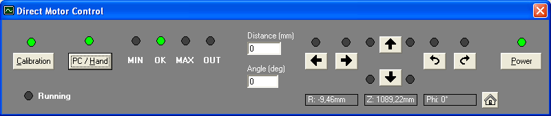   Motor Control device indicating that the Laser Signal is Ok

   The distance for the Ok point is about 25 mm from the lower edge of the Keyence LK-G32 Laser Head. Use the Motor Control to adjust the Z height until the green Ok LED is glowing.

10. Try to increase the diffuse reflectivity of the speaker surface in case no proper Laser Signal can be measured

11. Start a new scanning project (see section Start new Scan)

    Open the TRF Setup and perform a Test Measurement.

12. In case the Test Measurement did not succeed, please save the TRF operation in a Klippel database file using the Save Operation… button of the TRF Setup dialog and contact support@klippel.de with the database file as email attachment.

Error Messages

The error messages of the Klippel Scanning System are described here and remedies are suggested.

Available Devices

A Klippel device with proper license files for the requested operation has to be connected and switched on.

Refer to the description of Klippel Licences.

Critical Error

Please contact support@klippel.de in case you get this error message.

Desired excitation level cannot be realized

This error message is generated if the amplifier gain is too small to realize the desired excitation level.

Remedy: Increase the amplifier gain. Decrease the stimulus voltage to the value shown in the message box.

Keyence Laser Controller Error

To assure a correct programming of the Keyence Laser Controller a serial connection between the measurement PC and the Laser Controller is required; see also section Setup of the Scanning System.

If no connection over a serial cable can be detected, then a correct laser vibration measurement cannot be guaranteed.

The Laser Controller has to be switched on and the red laser beam has to be visible.

Remedy: Check the serial cable between PC and Laser Controller. Consult the manual section Setup of the Scanning System.

Keyence Laser Sensor Error

Laser Sensor control LED at its backside flashes but no laser light will be emitted. Ensure that the sensor will be connected before powering up the Laser Controller.

Remedy: Switch off the Laser Controller, check the connection between Laser Sensor and Laser Controller and switch on the Laser Controller again.

If the problem remains, see Keyence user manual or contact support@klippel.de.

Klippel Automation Error

The Klippel Scanning System requires a related installation of an appropriate Klippel dB-Lab. If the associated dB-Lab installation cannot be found or is broken, then the Klippel Scanning System cannot run anymore.

Remedy: Make sure that the associated dB-Lab Installation still exists and is working. This can be checked by the Start Menu Link “Klippel Analyzer -> Scanner -> Run dB-Lab”.

Reinstall an actual Version of the Klippel Scanning System to renew the broken association to the dB-Lab.

Motor Control Error

The Motor Control device can detect whether one of its cables is not properly connected. The simultaneous glowing of both end contact LED’s belonging to one scanner axis indicates that the respective motor axis is not properly connected.

Motor Control not connected to Z axis and R / Phi axis

Remedy: Check all connections between the Scanner Hardware and the Motor Control according to the section Setup of the Scanning System.

No proper amplifier output

The amplifier is switched off or the test signal is not transmitted properly.

Remedy: Check the amplifier and check the connections to the Analyzer hardware as described in the section Setup of the Scanning System.

See the TRF – Transfer Function Measurement for more information.

Scanner End Contact

This message occurs when the Scanner hardware has reached one of the end contacts. In case this happens during regular scanning operation, please conduct a complete Hardware Check and send the log file to support@klippel.de.

The Motor Control will not execute any driving command except a command moving away from the respective end contact.

Z Collision upwards

The Z-axis has reached the upper limit of its driving range.

Z Collision downwards

The Z-axis has reached the lower limit of its driving range.

R Collision at front side

The R-axis has reached the front limit of its driving range.

R Collision at rear side

The Z-axis has reached the rear limit of its driving range.

Phi Collision clockwise

The Turntable has reached the limit of its driving range in clockwise orientation.

Phi Collision counter-clockwise

The Turntable has reached the limit of its driving range in counter-clockwise orientation.

Laser Collision

The Laser Head has touched the surface of the scanned object.

Emergency Stop

An emergency end contact was reached. That means, one of the regular end contact switches has failed. Please contact support@klippel.de!

Scilab executable not found

The scripts for post processing the measured vibration data require an installed Klippel SciEngine. The former SciEngine installation cannot be found anymore.

Remedy: Reinstall the Klippel SciEngine from CD.

Script could not be started

Refer to the description of Klippel Licences.