TFA – Time Frequency Analysis

TFA Tutorial

Overview

TFA is a post-processing module dedicated to the time-frequency analysis of audio signals and impulse responses. It visualizes the signal level over frequency and time. In other words, it shows at which time which frequency gives a contribution to the signal power. For example, by analyzing the impulse response of a room, a resonance with low damping can be detected very easily. The method can also help to detect loudspeaker defects (Rub & Buzz) and visualizes very clearly at which frequencies these problems appear. The TFA module enables the user to select the range at which these problems appear and listen to exactly that part of the audio signal.

What is the Goal of This Tutorial?

This tutorial makes you familiar with the TFA module.

The tutorial has four parts:

1. In Part 1 - Viewing TFA Results we will show you how to view and interpret TFA results which are already stored in the web example database.

2. Part 2 - Wavelet Transform of Impulse Response guides through a specific application; the Wavelet transform of an impulse response measured by the TRF – Transfer Function Measurement module. It shows how to do a time frequency analysis step by step and how to modify the settings to find the best configuration.

3. Part 3 - Analysis of Long Wave Files introduces the handling of long audio signals (e.g.: recording of a speaker reproducing a song). It gives an introduction on how to identify the interesting parts of a long audio signal and how to analyze, listen to and export them.

4. The usage of the TFA module for playing back a signal only is explained in Part 4 - Using the playback functionality exclusively.

Part 1 - Viewing TFA Results

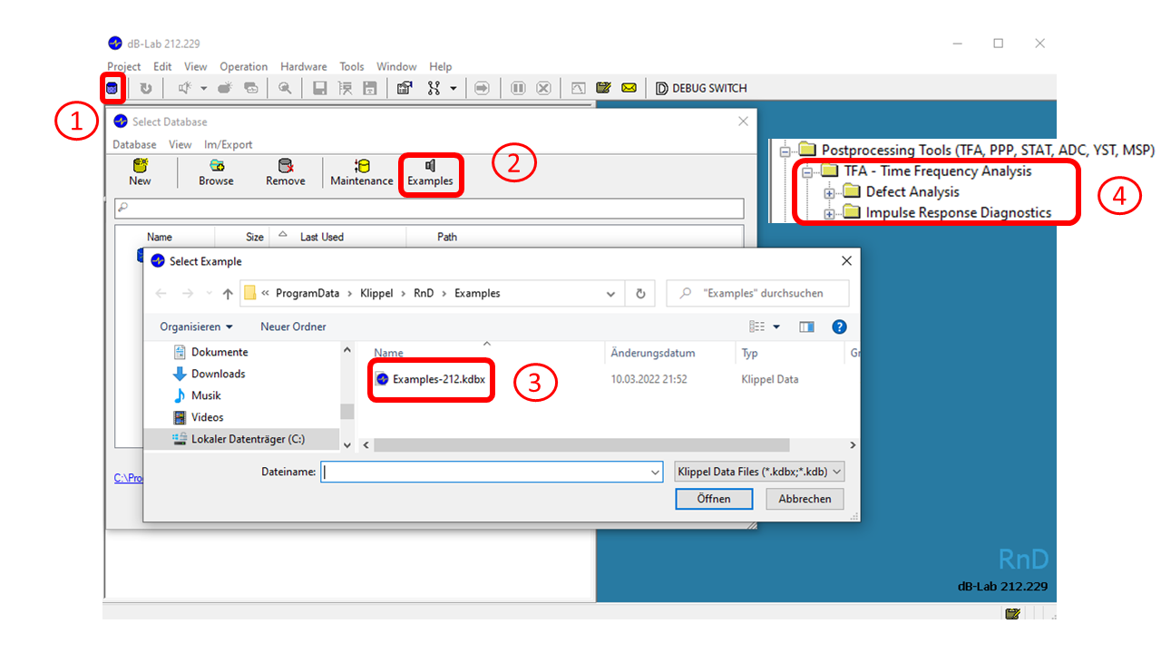
Example data used in this manual is stored in the Web Example database. If not downloaded already, get it from the latest R&D release <https://www.klippel.de/go/current-rnd-release> and open the web-based database.

See also

View Results for general information on how to download this database, open and view results in dB-Lab.

Open the folder Postprocessing Tools (TFA, PPP, STAT, ADC, YST, MSP) \TFA - Time-Frequency Analysis

Defect Analysis

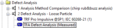
Open the database folder Defect Analysis and in the object 2 Defect Analysis – Loose Particle the operation TFA Defect Analysis (Measured).

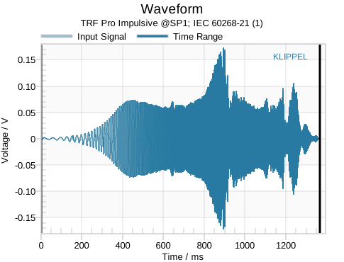
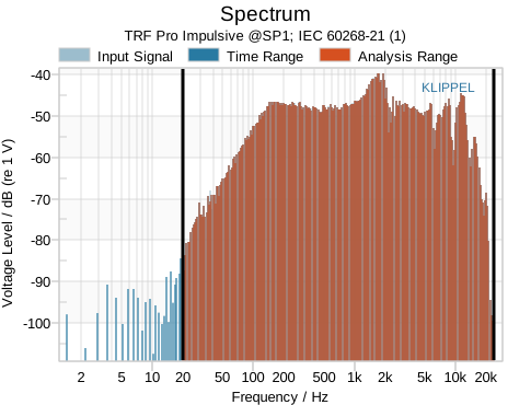
Double clicking the operation will open the default windows. The window Waveform and Spectrum show the time signal and the spectrum of the measured microphone signal of the TRF operation. The time and frequency cursors in the plots show the selected range for the analysis. Additionally, the window Waveform (Time Range) provides a detailed view of the time range selected in the window Waveform.

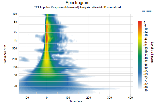
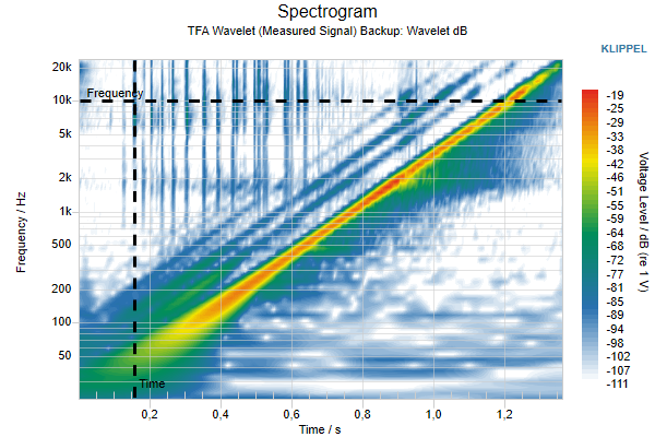
Now take a look at the Spectrogram (Analysis Range) window. This graph shows the level (color) over time (abscissa) and frequency (ordinate). The TRF measurement is using a logarithmic sweep as the stimulus. As seen in the picture, the frequency of the fundamental increases logarithmically with time. The “regular” lower-order harmonic distortions appear in the spectrogram above the fundamental as lines which are parallel to the fundamental. In this example the 2^nd and 3^rd order harmonic distortions are very distinct. From \(t \approx 100\ \text{ms}\) to \(t \approx 650\ \text{ms}\) vertical lines in the spectrogram can be seen. These vertical lines clearly indicate a loose particle defect.

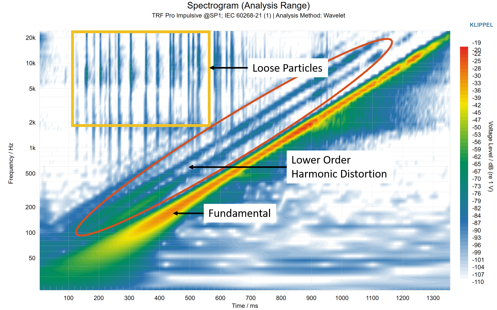
Also see the other examples of loudspeaker defects in the database (e.g. Voice Coil Bottoming, Leakage or Music Rub & Buzz). Each defect shows a different picture in the signal level distribution over time and frequency.

By clicking the Enable Bandpass Filter checkbox the area in the Spectrogram (Analysis Range) window displaying Rub & Buzz can be selected and played back.

Waterfall Spectrum

For this part of the tutorial another signal is analyzed. Select the folder Impulse Response Diagnostics and the object 2 Waterfall Analysis – Speaker Room Interaction. Then select the operation 2 TFA – In Situ (Original).

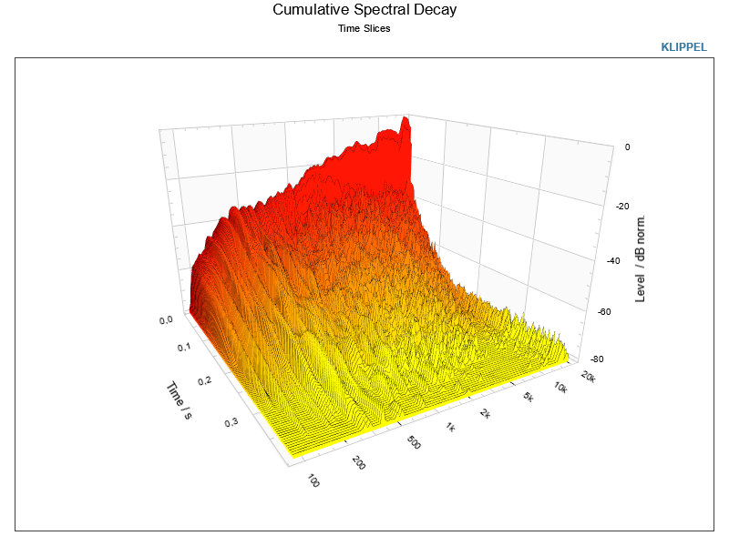
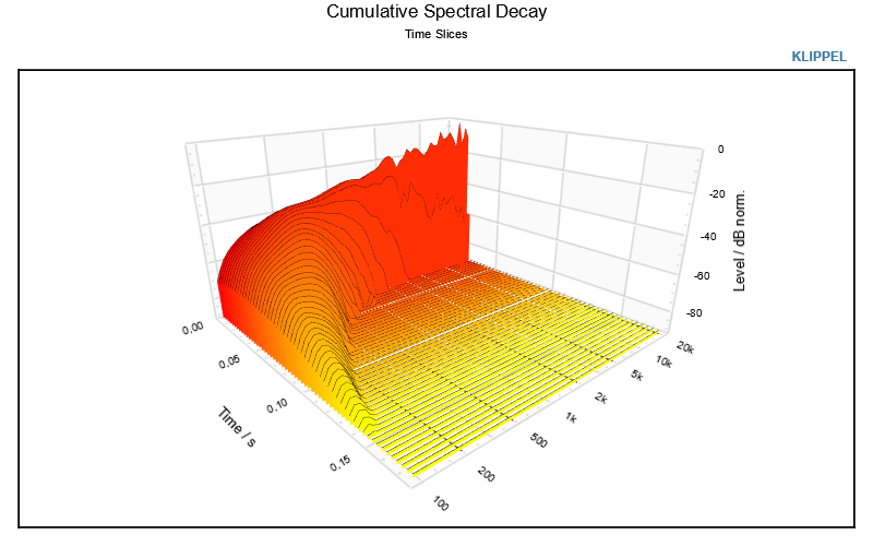
The result called “2 TFA – In Situ (Original)“ is a measurement of the loudspeaker’s impulse response in a normal office room. The result window 3D Plot is a 3D representation of the Spectrogram (Analysis Range) window and shows how much the speaker excites the room over time. At low frequencies there are distinct narrow-band resonances in the room that have a low damping and a long ringing. At higher frequencies also an influence of the early reflections and the reverberation of the room is visible, but the higher frequencies have higher damping and thus a faster decay.

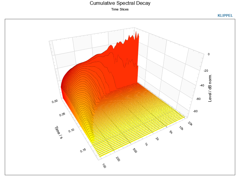
By using a compensation filter to remove the room effects, the simulated free field response of the loudspeaker can be calculated, which is shown in the operation called “3 TFA – Direct Sound Only”. As seen in the 3D Plot window, the room was removed and the loudspeaker system, which has a much faster decay.

Part 2 - Wavelet Transform of Impulse Response

In the object 1 Free-field Speaker impulse response select the operation TFA Impulse Response (Measured) Analysis.

Data Import

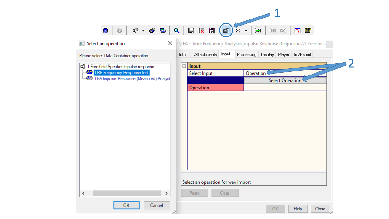
1. Open the Property Page of the selected operation

2. Select the operation TRF Frequency Response test as the Input

3. Select the window h(t) Impulse Response

4. Select the curve Measured

5. Click Import to load the Impulse Response into the TFA module

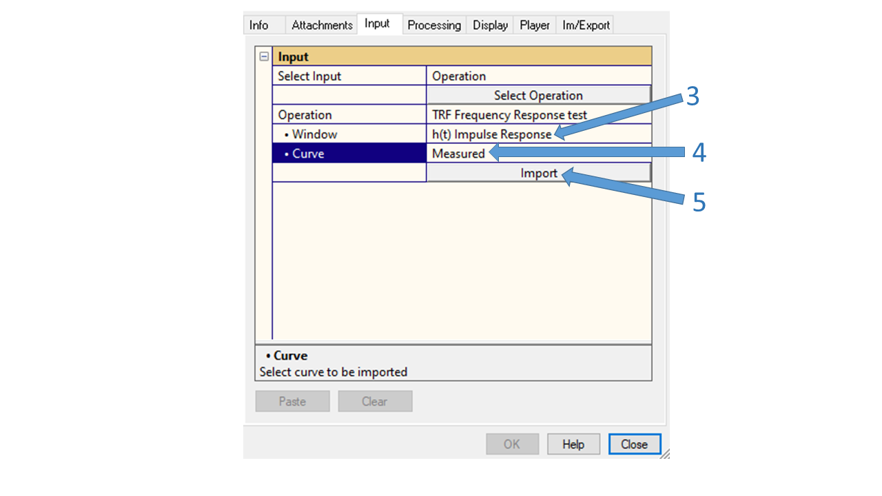
After the import, the name of the operation is shown under Select Input.

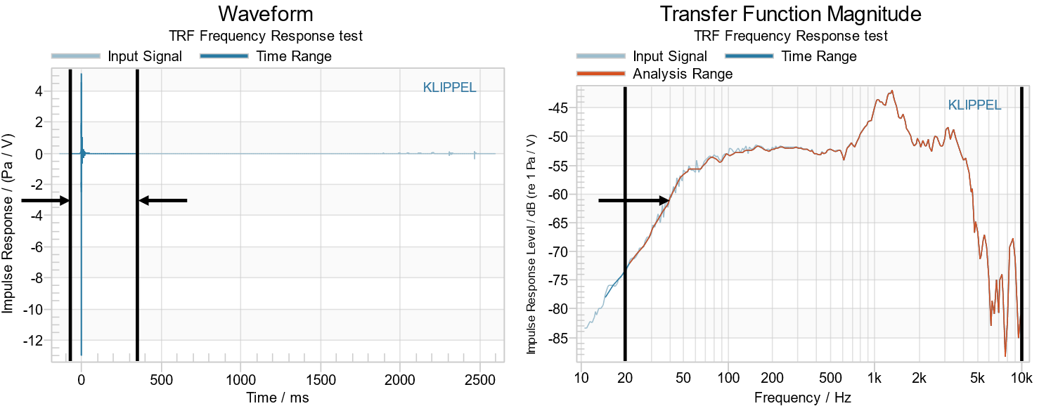
The impulse response and the transfer function are shown in the windows Waveform (view of the full imported impulse response), Waveform (Time Range) (view of the selected time range) and Transfer Function Magnitude.

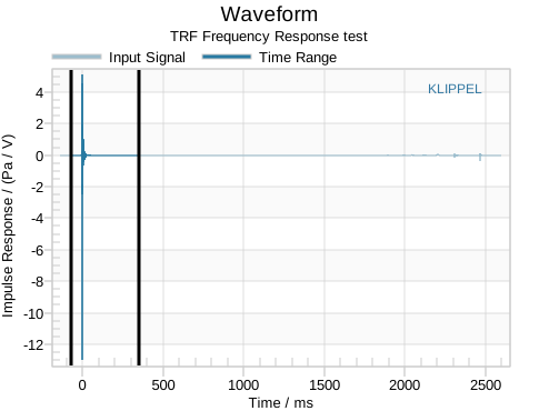
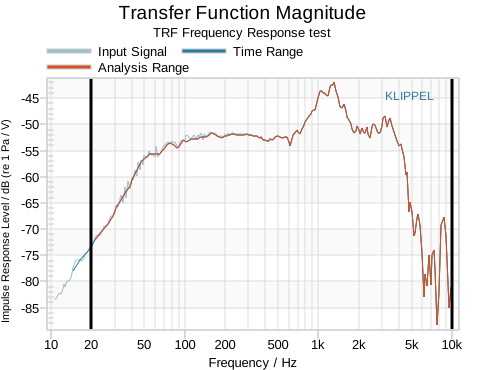
Click and drag the left and right cursor of the Waveform window to select the time range for the time-frequency analysis. After adjusting the cursors positions, the windowed spectrum will be updated. In addition, the cursors of the Transfer Function Magnitude window can be used to limit the frequency range of the analysis.

Configuration of the Wavelet Transform

Open the Analysis category of the Property Page and select the Wavelet transform as Analysis Method.

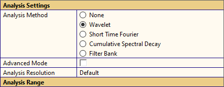
By default, the Advanced Mode is deactivated and a choice between three Analysis Resolutions is offered. The Default setting provides a good compromise between time and frequency resolution. If a higher frequency resolution is required, the Analysis Resolution Frequency Priority is provided. This setting is beneficial for the identification of resonance frequencies. If a higher time resolution is required the Analysis Resolution Time Priority is provided. This setting is beneficial for impulsive distortion analysis.

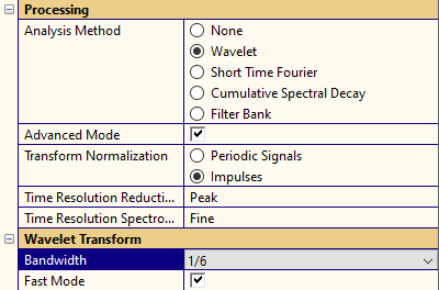
When activating the Advanced Mode, the settings for the chosen Analysis Method are shown. For the Wavelet Transform the Bandwidth is adjusted to satisfy a higher time or frequency resolution. Additionally, the Transform Normalization is set to Impulse (see: Transform Normalization for more information).

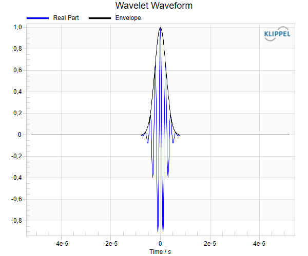
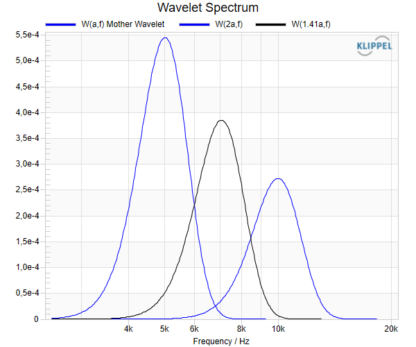
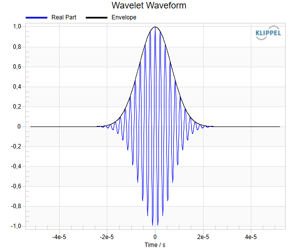
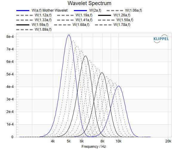
Open the windows Wavelet Waveform and Wavelet Spectrum windows to see the characteristics of the mother wavelets. The decreasing amplitude of the wavelets is caused by the wavelet normalization for impulses.

Bandwidth = 1/2 octave

Bandwidth = 1/6 octave

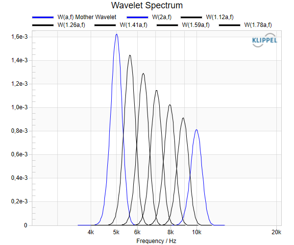
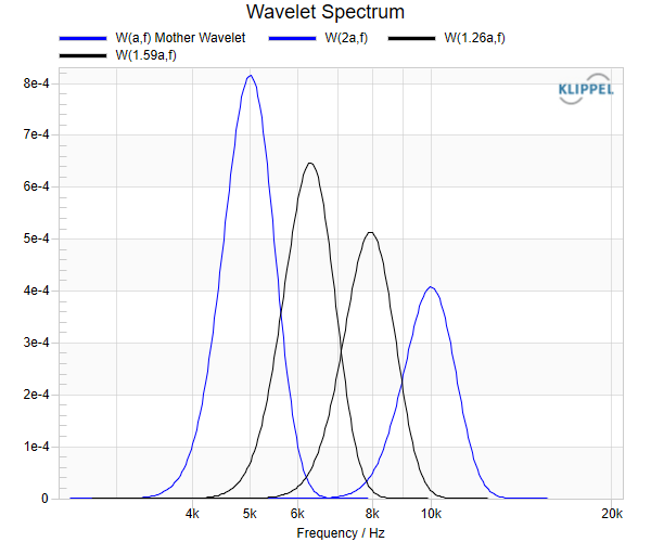
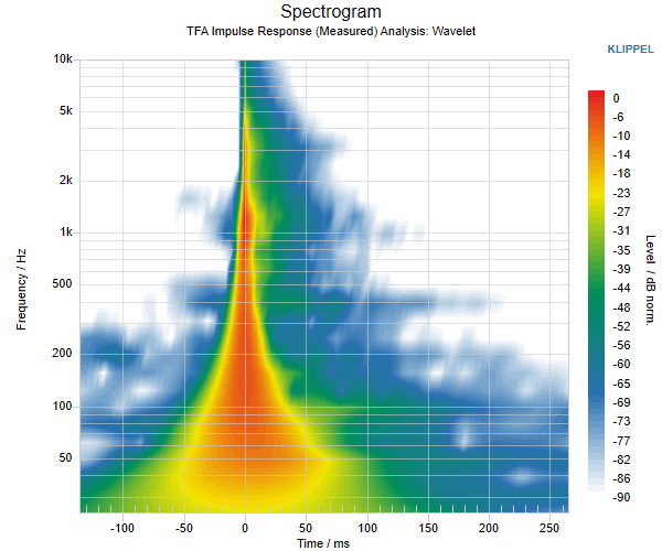
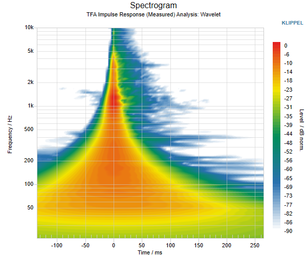
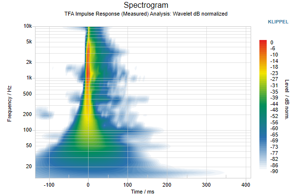
By deactivating the Fast Mode, additional wavelets are calculated within the band to minimize artifacts and get smoother and sharper visualization results concerning the frequency resolution.

☑ Fast Mode

☐ Fast Mode

Set the Bandwidth to 1/3 octave, deactivate the Fast Mode and run the operation.

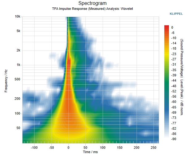
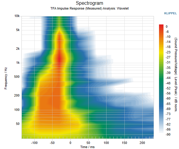
Additionally, the Advanced Mode provides an adjustable Time Resolution Reduction for the Spectrogram (Analysis Range) window. This resolution reduction of the spectrogram comes with two Time Resolution Reduction Modes which influence the signal levels over time and frequency. The RMS mode reduces the time resolution by calculating the root mean square of a time interval, thus this mode is suitable for evaluating signal energy.

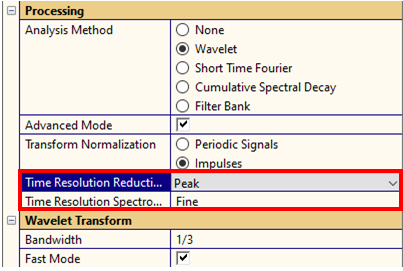
The Peak mode reduces time resolution by searching for the peak value of a time interval. This mode is especially useful when analyzing impulsive properties of an audio signal. The Time Resolution Reduction can remain on the default setting Fine for the analysis of impulse responses.

Time Resolution Spectrogram = Fine

Time Resolution Spectrogram = Medium

Results

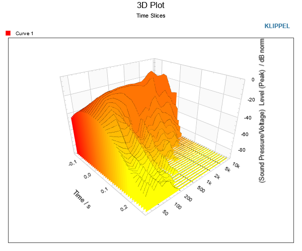
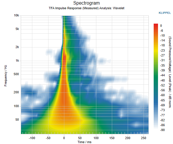
Open the result windows 3D Plot and Spectrogram (Analysis Range) to analyze the decay of the signal level over time and frequencies.

Open the Property Page and select the Category Display Using the parameters of this section the result windows can be modified to optimize the visualizations.

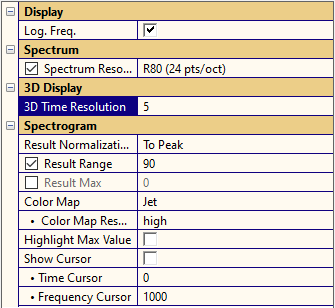
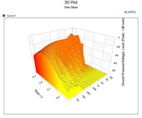
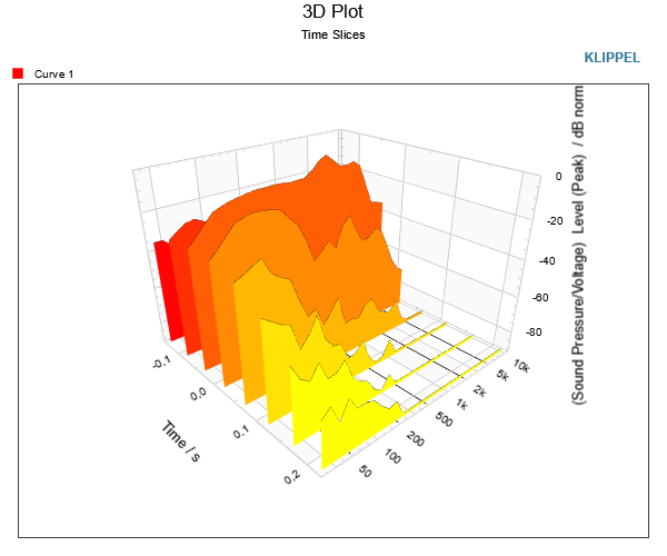
For example, you can modify the parameter 3D Time Resolution to adjust the time resolution of the waterfall spectrum.

3D Time Resolution = 5 ms

3D Time Resolution = 50 ms

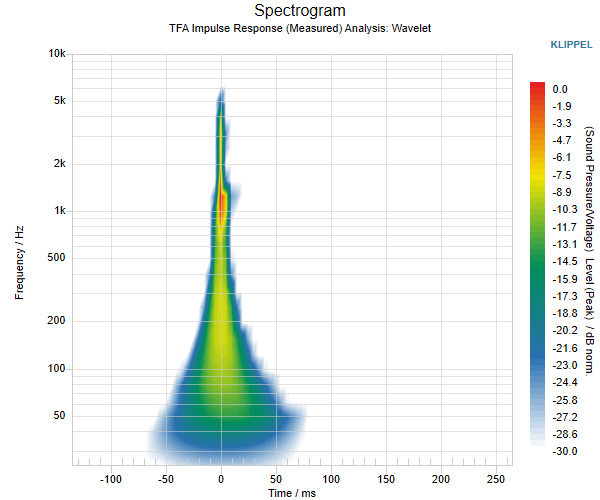
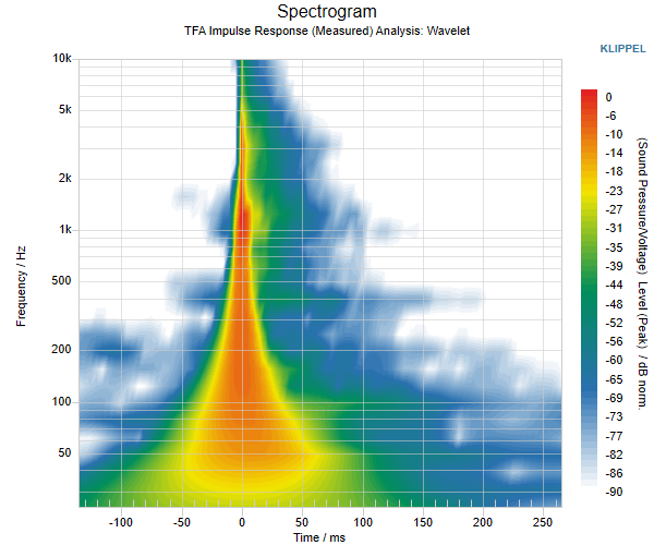
For the Spectrogram (Analysis Range) window the Result Range can be modified as well as the Color Map settings including the Color Map Resolution.

Result Range = 100 dB

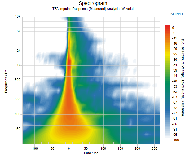
Result Range = 30 dB

Color Map Resolution = Low

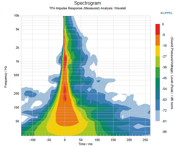
Color Map Resolution = High

Part 3 - Analysis of Long Wave Files

Selecting the Part of Interest

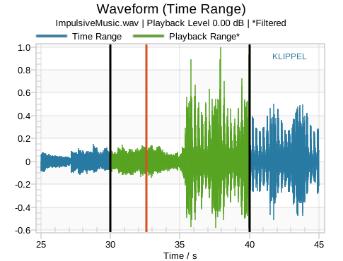
When a long audio signal is imported, the signal will be displayed as a bar graph in the window Waveform. By default, a time range in the middle of the imported audio signal is chosen for the analysis. The selected time range is shown in the Waveform (Time Range) window in greater detail.

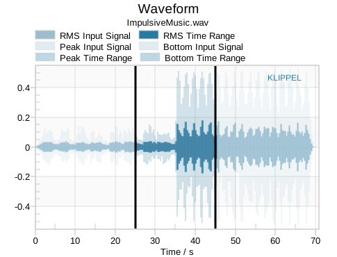
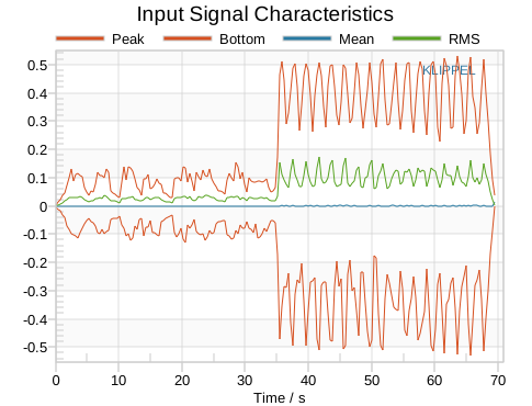
The window Waveform provides the peak, bottom and root mean square (RMS) values of time intervals of the imported long audio signal. High peak or bottom values can help to identify parts in the audio signal with impulsive signal components (e.g., Rub&Buzz). High RMS values can help to identify parts with high signal energy that may trigger nonlinear distortion.

Open the window Input Crest Factor. The maximum values of the crest factor correspond to the highest ratio between the peak value and the root mean square in a time interval. Thus, a high crest factor may give clues to find impulsive distortion in a signal.

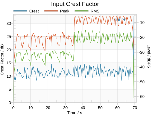
Use the cursors of the window Waveform to select the time range containing the highest crest factor of the signal. In the Waveform (Time Range) window a detailed view of the selected time range is displayed.

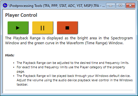
Use the cursors in the Waveform (Time Range) window to select the playback time range. Press the Play button in the Player Control window to start the playback. Press the Stop button to stop the playback.

Select the Wavelet transform, use Default as Analysis Resolution and run the operation.

Using the Bandpass Filter

In the property page Player click the checkbox Enable Bandpass Filter. This setting enables user to select a time and frequency range for the playback in the Spectrogram (Analysis Range) window. The selected time and frequency range is displayed as a transparent colored rectangle. With the cross cursors the time and frequency range selection can be altered. The cursors can be dragged with the mouse or clicked (Shift + left mouse button for the lower limit, CTRL + left mouse button for the upper limit and ALT + left mouse button for the play position). Select the area indicating a defect and press the Play button to listen to the filtered signal.

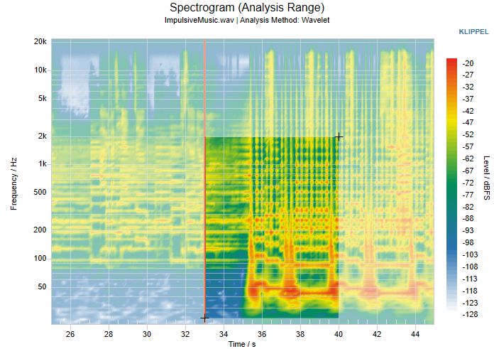
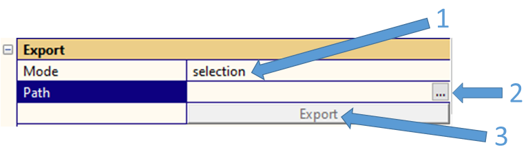
The selected time and frequency range of the imported audio signal may be exported using the export functionality in the property page Player. In the category Export select the Mode Selection to export the selected time and frequency range. Choose a path and a name for the exported signal by clicking on Path. Finally click Export to execute the export.

Part 4 - Using the playback functionality exclusively

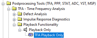
Open the database folder Playback Functionality and in the object Playback Only the operation TFA Playback Only.

Import Waveform

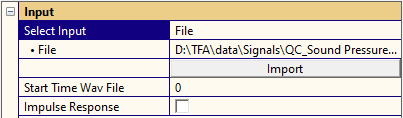
The first step is to import a waveform. The waveform may be imported using any of the provided choices of the parameter Select Input. Here, a file is imported. To do so, select the import choice File. Then enter or select the path to the wave file using the parameter File. Then click the Import button to import the specified file.

Settings

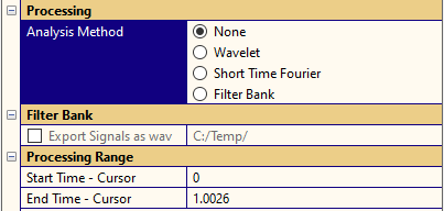
Go to the property page Analysis. Select the Analysis Method None. This way, only relevant windows and parameters are shown.

Note

Using the Analysis Method None, the playback functionality can be used without a licence.

The player settings can be altered using the property page Player. The Input Level parameter shows the relative peak value of the input file. The playback level can be normalized with the checkbox Normalize Playback Level or adjusted to a user defined value in dB with Set Playback Level. The signal may be slowed down using the Playback Rate and may even be bandpass filtered. The bandpass filter can be activated using the Enable Bandpass Filter checkbox. The played back waveform will then be bandpass filtered as specified.

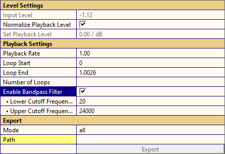
The loop start and stop times can be specified using the parameters Loop Start and Loop End. This can also be done by using the cursors in the Waveform (Time Range) window. The number of times the loop is played can be specified using the parameter Number of Loops. If the parameter Number of Loops is empty the playback will be looped until stopped by the user.

Note

If the TFA module is used as a player in a batch and the parameter Number of Loops is empty, the loop will only be played once.

Player Control

The player may be started using the Play button in the Player Control window or using the run button. The playback can be stopped using the red cross or using the Player Control buttons Pause and Stop.

TFA Reference

Overview

The time-frequency analysis is a common method for analyzing the spectral content of audio signals over time. Similar to a music sheet it visualizes which frequencies are dominant at which time.

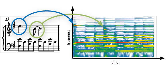
Based on four different methods, the Wavelet Transform (WT), the Short Time Fourier Transform (STFT), the Cumulative Spectral Decay or a Bark scaled Filter Bank Analysis (FBA), the TFA decomposes the input signal and visualizes the signal characteristics over frequency and time.

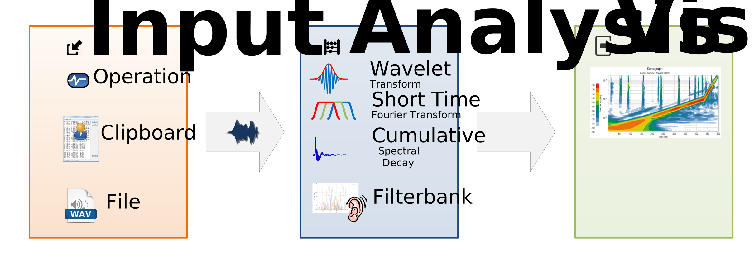
Analysis

Wavelet Transform

The Wavelet Transform (WT) is based on Gaussian wavelets. While the STFT has a static time and frequency resolution defined by the window function, the WT uses wavelets with constant octave bandwidth for every frequency band. This makes the WT perfectly suitable for analyzing a broad frequency at sufficient time resolution.

\[Y^{\psi}(a,b) = \left| \frac{1}{\sqrt{\left| a \right|}}\int_{- \infty}^{\infty}{x\left( t \right)\psi^{*}\left( \frac{t - b}{a} \right)\text{d}t} \right|^{2}\]

The wavelets \(\psi^{*}\left( \frac{t - b}{a} \right)\) are normalized ensuring that the audio signal’s level at a certain frequency and time equals the level shown in the spectrogram at that frequency and time if the Transform Normalization is set to Periodic Signal. Thus the amplitude of the wavelets \(\psi^{*}\left( \frac{t - b}{a} \right)\) is equal to one in the freuency domain. If the Transform Normalization Impulses is used, the amplitude of the wavelets \(\psi^{*}\left( \frac{t - b}{a} \right)\) are equal to 1 in the time domain.

The WT also calculates the signal’s group delay, which expresses when the mean energy in a frequency band arrives. It is mainly useful when analyzing impulse responses, since it shows delays due to resonances, for instance.

\[t_{x}\left( f \right) = \frac{\int_{- \infty}^{\infty}{t \cdot Y^{\psi}\left( f,t \right)\text{d}t}}{\int_{- \infty}^{\infty}{Y^{\psi}\left( f,t \right)\text{d}t}}\]

Short Time Fourier

The Short Time Fourier Transform (STFT) is the most common method applied for time-frequency analysis. It can be configured through window type, length and overlap settings. The selected window function \(h\left( t \right)\) is normalized ensuring that the audio signal’s input level at a certain frequency and time equals the level shown in the spectrogram at that frequency and time if the Transform Normalization is set to Periodic Signal. If the Transform Normalization Impulses is used, the amplitude of the window function is equal to 1 in the time domain.

\[Y\left( t,f \right) = \left| \int_{- \infty}^{\infty}{e^{- j2\pi f\tau}x\left( \tau \right)}h\left( \tau - t \right)\text{d}τ \right|^{2}\]

Cumulative Spectral Decay

The Cumulative Spectral Decay shows the power contained in an impulse response \(h(t)\) in the frequency domain windowed with a shifted Heaviside step function \(u(t)\) over time. The impulse response \(h(t)\) is cut beginning with the first samples. Thus, the cut samples do not contribute anymore to the power of the impulse response. The shift increment of the Heaviside step function \(u(t)\) can be adjusted and corresponds to the time resolution of the Cumulative Spectral Decay. Additionally, the Heaviside step function \(u(t)\) may be expanded by half a window function (von Hann, Hamming and Triangle) to reduce artifacts that occur because of the Heaviside step function. The rise time of the window function expanding the Heaviside step function may also be adjusted.

\[\left| Y(t,\omega ) \right|^{2} = \left|\mathcal{F} \{ u(t-\tau ) h(\tau ) \}\right| ^{2}\]

Filter Bank

The filter bank analysis (FBA) separates spectral components using multiple auditory band-pass filters. The center frequencies are evenly distributed over a Bark frequency scale (roughly logarithmic). This calculation method applies a perceptual time-frequency analysis. The filter bank analysis is able to visualize short-time effects such as impulsive noise or the fluctuation of an amplitude-modulated signal. The time resolution in lower frequencies is the best of all of the other methods. Additionally, the filters are normalized ensuring that the audio signal’s level at a certain frequency and time equals the level shown in the spectrogram at that frequency and time. Thus this method is not recommended for the analysis of impulses.

Parameters

Input

Input

Select Input

The parameter specifies from where the data will be imported. Values are:

File

Absolute or relative path to a wave file

Note

The full waveform is displayed as a bar chart for wave files exceeding a length of 21 s with a sampling frequency of 48 kHz. The bar chart contains the peak, bottom and RMS values for time intervals.

Directory

Absolute or relative path to a directory containing wave files

Enter the directory and a select-list will appear with the available files.

Note

The full waveform is displayed as a bar chart for wave files exceeding a length of 21 s with a sampling frequency of 48 kHz. The bar chart contains the peak, bottom and RMS values for time intervals.

Clipboard

Paste waveform curve from other operations or external sources

Note

The time axis of imported signals is checked for an equal spacing of the samples upon import. If the spacing of the time axis (sampling period) deviates more than 50% a warning is generated and the time axis will be reconstructed at the mean value of the spacing of the time axis.

Operation

Import waveforms from other supported operations. An operation can be selected by clicking the Select Operation button or by typing the name of the operation into the Operation parameter. When an operation is selected, the select-list Window shows all the available windows to import data from. Allowed windows have the keywords “Waveform” or “Impulse Response” in their titles. After the selection of a window, the select list Curve shows all the curves inside the selected window.

Note

The time axis of imported signals is checked for an equal spacing of the samples upon import. If the spacing of the time axis (sampling period) deviates more than 50% a warning is generated and the time axis will be reconstructed at the mean value of the spacing of the time axis.

Imported

Select already imported data as input

Channel

Select the channel of the selected wave file for import.

Start Time Wav File

A start time can be specified for wave file import. This is useful if it is already known that the beginning of a wave file is not of interest.

Impulse Response

This checkbox can be activated when an imported wave file or data imported via clipboard shall be interpreted as an impulse response. This setting is hidden for Operation import since the import of an impulse response using the Operation option is detected automatically. Upon activation of this checkbox only result windows and result curves suitable for the analysis of an impulse response are displayed. The window Spectrum is replaced by the Transfer Function Magnitude window.

Note

When importing an impulse response from a TRF operation via operation import, the displayed maximum value may be larger in the TFA module compared to the TRF operation. This difference is caused by a down sampling in the display of the TRF operation.

Store File

Upon activation of this checkbox the complete wave file is stored in the attachment of the operation. This checkbox is activated by default. Deactivate this option to reduce the needed amount of memory for the operation. When deactivated, only the part of the wave file within the time range is stored in the attachment of the operation. When sending this operation to another dB-Lab user, he may not alter the time range if the Store File checkbox is deactivated, since the rest of the wave file might not be available.

Note

The parameter Store File is only shown if a wave file with a length exceeding 21 s at a sampling frequency of 48 kHz is entered in the parameter File (see: Select Input).

Analysis

Analysis

Analysis Method

None

Usage of this mode is recommended if the TFA module is used as a player. No licence is needed to use this mode. No analysis will be performed upon pressing run button but the playback will be executed. All the windows and settings that are not related to the playback functionality are hidden.

Wavelet

This mode requires a licence. A Wavelet analysis will be performed upon pressing the run button. The wavelet transform offers a logarithmic frequency resolution. Additionally, the time resolution increases with frequency.

Short Time Fourier

This mode requires a licence. A short time Fourier analysis will be performed upon pressing the run button. The short time Fourier transform offers a linear frequency resolution which is beneficial when analyzing the higher order distortion components of a signal. The time resolution depends on the chosen window length and the overlap. A shorter analysis window will result in a poorer frequency resolution, while obtaining a high time resolution.

Cumulative Spectral decay

This mode requires a licence and is only allowed for the analysis of impulse responses. The cumulative spectral decay will be calculated upon pressing the run button. The cumulative spectral decay offers a linear frequency resolution which is reduced to a logarithmic frequency resolution and helps to analyze the power decay of an impulse response over time and frequency.

Filter Bank

This mode requires a licence. A filter bank analysis will be performed upon pressing the run button. The filter bank has the best time resolution at low frequencies compared to the other analysis methods. The filter bank offers a perceptual analysis of the signal.

Advanced Mode

The Advanced Mode checkbox is recommended for users with some experience in the field of time frequency analysis and offers more detailed settings to tune the analysis in the preferred way. Tuning the analysis can be required since the time frequency analysis is always a compromise between time and frequency resolution.

The Advanced Mode is deactivated by default. In this case the user may choose between three Analysis Resolutions:

Frequency Priority

This setting offers a higher frequency resolution and is recommended for signals containing dense frequency information that does not change fast.

Default

This setting offers a compromise between time and frequency resolution.

Time Priority

This setting offers a higher time resolution and is recommended for the analysis of transient behavior (e.g.: impulsive distortion).

Additionally, the time resolution settings of the Spectrogram (Analysis Range) and the 3D Plot windows are hidden when the Advanced Mode is deactivated.

Transform Normalization

The parameter Transform Normalization changes the normalization of the analysis windows of the Wavelet Transform and the Short-time Fourier Transform. The user may choose between two options:

Periodic Signals

The level of a periodic signal will be displayed correctly in the spectrogram. The maximum value of the transfer function of the analysis windows will be equal to 1.

Impulses

The level of an impulse will be displayed correctly in the spectrogram. The maximum value of the impulse response of the analysis windows will be equal to 1.

Note

The parameter Transform Normalization is only visible if the Advanced Mode checkbox is activated and the Analysis Method Wavelet or Short Time Fourier is selected. If the Advanced Mode is deactivated, the Transform Normalization is set automatically depending on the imported signal. If the signal is an impulse response (automatically detected using the import option Operation or by activation of the checkbox Impulse Response) the parameter Transform Normalization will be set to Impulse. Otherwise it will be set to Periodic Signal.

Time Resolution Reduction Mode

This parameter is only visible for the wavelet transform and the filter bank since the time resolution of both analysis methods is reduced to limit plot data size. The user may choose between two calculation modes:

RMS

Calculation of the root mean square of a time interval.

Peak

Searching for the peak value of a time interval. Recommended for the analysis of transient behavior.

Time Resolution Spectrogram

The user can choose between three predefined time resolutions or specify a custom time resolution. The predefined time resolutions are:

Coarse

500 ms

Medium

50 ms

Fine

5 ms

QC 3DL Spectrogram

Same resolution as the QC 3DL Spectrogram

Custom

A custom resolution may be entered in ms

Note

For very short analysis ranges the setting Coarse might be too long. In this case the maximum allowed resolution is used. For very long analysis ranges the setting Fine might be too short and will be set to the allowed minimum value. The value has to be entered in ms.

Wavelet Transform

Bandwidth

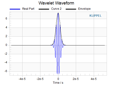
Wavelets have a constant octave fraction bandwidth which affects the time resolution of the used wavelets. With a high bandwidth the wavelet will be sensitive for short effects like impulses and defects. Smaller bandwidths (< 1/4 octave) are used for detecting resonances.

The effect of this parameter is illustrated in the windows Wavelet Waveform and Wavelet Spectrum.

Bandwidth = 1/2 octave

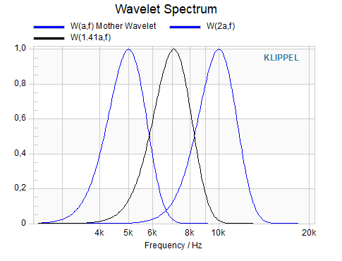
Bandwidth = 1/6 octave

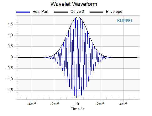
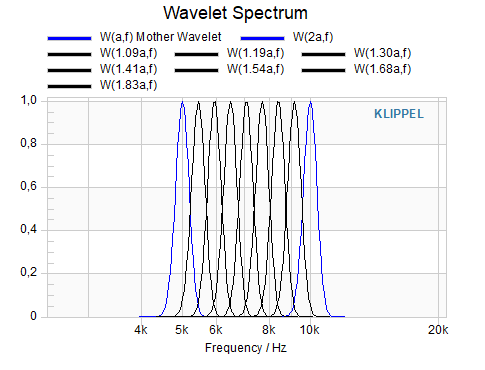
Fast Mode

Fast Mode uses fixed wavelet center frequencies that may generate artifacts at the intersection with neighboring wavelets. If disabled, the result will be calculated much smoother, but the analysis time will increase. The Fast Mode setting is only available for Bandwidths smaller then 1/8 octave.

When analyzing impulse responses, the Fast Mode should usually be turned off.

☑ Fast Mode

☐ Fast Mode

Short Time Fourier Transform

Window Type

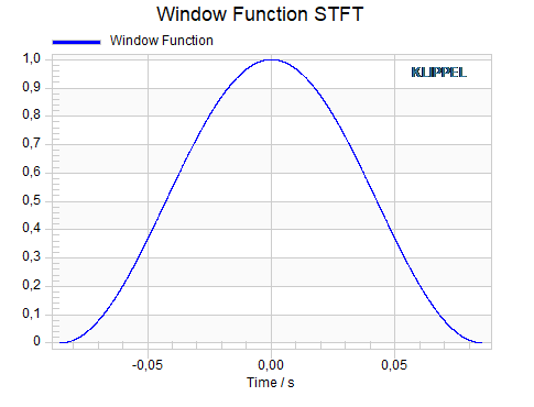
Define the window function used for the STFT analysis. Check the Window Function STFT window to take a look at the graphical representation.

Window Time

This parameter defines the length of the applied windowing. Have a look at the Table Results + Settings window for detailed information about the resulting frequency resolution and the window length in samples. Short window times make the system sensitive to short effects like impulses (better time resolution). A long window should be used for more exact frequency information (better frequency resolution).

Window Overlap

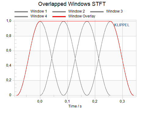
This value given in percent defines the window overlap. The recommended value list provides typical values but it is also possible to define a Custom Overlap value or give an implicit definition of window overlap with a Custom Number of Slices. You can use a high overlap for a smoother spectrogram in time direction. However, analysis time may increase significantly with high overlap values.

Check the Overlapped Windows STFT window for a graphical representation of the Window Overlap. The Table Results + Settings window will give you information about the resulting window shift (time/samples) and the total number of slices.

Cumulative Spectral Decay

Window Type

Set the desired window type expanding the Heaviside step function used in the calculation. The expansion of the Heaviside step function reduces artifacts that occur because of the Heaviside step function by making the edge smoother. The user may choose between three options:

1. von Hann

2. Hamming

3. Triangle

If the Advanced Mode is deactivated, the von Hann window function is used.

Rise Time

Set the desired rise time of the window function expanding the Heaviside step function. A long rise time will decrease the time resolution while a short rise time will introduce more artifacts.

Note

If the Rise Time is set to 0 the Heaviside step function will not be expanded by an additional window function.

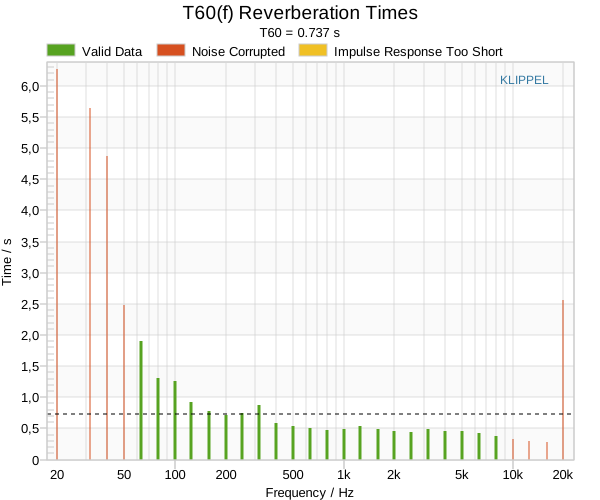
Calculate T60

Ticking this checkbox activates the reverberation time T60 calculation. The reverberation time describes the time needed for the energy of the impulse response in a given band to decay by 60 dB. The reverberation time is calculated globally (over all bands) on the basis of the Energy Time Curve and frequency dependent using the Cumulative Spectral Decay analysis results. The algorithm differentiates between valid and invalid (SNR too low or impulse response too short) measurements. To get valid results set the Start Time - Cursor shortly after the main impulse of the room impulse response in the linearly decaying part of the Energy Time Curve. The End Time - Cursor should be set in flat range of the Energy Time Curve right after the knee of the Energy Time Curve in order to get the least amount of distortion.

Hint

Tick the checkbox Automatic Time Range to set the cursor positions automatically.

Note

In order to get the best results the measurement of the room impulse response should contain the least possible amount of direct sound. Thus, it is recommended to place the microphone in the far-field behind the speaker stimulating the room. A high SNR in every band can be achieved by using a full band speaker at high amplitudes.

Automatic Time Range

Ticking this checkbox will set Analysis Range used for T60 calculation automatically. The positions of the Start Time - Cursor and of the End Time - Cursor will be set in a way that achieves a good SNR. Ticking this checkbox is recommended to get an initial setting of the Analysis Range. But the best results will be yielded by fine-tuning the automatically set Analysis Range.

Filter Bank

Number of Filters

Set the number the band-pass filters defining the Filter Bank. The center frequencies are defined by the perceptual Bark scale. More filters lead to a better frequency resolution. Thus, the cost is a lack in time resolution and the analysis time will increase significantly.

Analysis Range

Start Time - Cursor, End Time - Cursor

These two parameters define the time range for analysis. The parameters can be set in the Property Page or by shifting the time markers in the Waveform window.

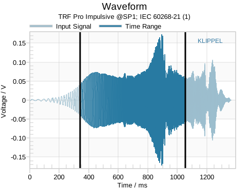
When a long audio signal (see Input) is imported, the signal will be displayed as a bar graph in the window Waveform. In this case the window Waveform provides the peak, bottom and root mean square (RMS) values of time intervals of the full audio signal.

Frequency Min - Cursor / Frequency Max - Cursor

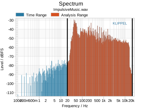
These properties allow to restrict the frequency range for the analysis. The parameters can be set in the Property Page or by shifting the cursors in the Spectrum window. For each Analysis Method there is a minimum analysis range defined by the bandwidth of the filters and window functions.

Display

Display

Log. Freq.

When activated, logarithmic frequency axes are used in all result plots.

Spectrum

Spectrum Resolution Reduction

If enabled, the resolution of the Spectrum and Transfer Function Magnitude windows are reduced. The reduction can be done according to ISO 266 standard frequencies or by a user defined resolution in frequencies per octave. After resolution reduction the frequencies will be logarithmically spaced.

R10 (3 pts/oct)

3 points per octave at preferred frequencies according to ISO 266

R20 (6 pts/oct)

6 points per octave at preferred frequencies according to ISO 266

R40 (12 pts/oct)

12 points per octave at preferred frequencies according to ISO 266

R80 (24 pts/oct)

24 points per octave at preferred frequencies according to ISO 266

By resolution (ref. 1 kHz)

User defined resolution in points per octave using standardized frequencies (reference 1 kHz)

3D Display

3D Time Resolution

Set the time resolution of the 3D Plot window. The allowed minimum value depends on the Time Resolution Spectrogram parameter.

If the Analysis Method is set to Short Time Fourier, the allowed minimum value is defined with the Window Overlap and Window Time parameters.

Spectrogram

Result Normalization

With this option, the results can be normalized to 0 dB. There are four options available:

None

No normalization

To Peak

The results will be normalized to the overall peak level of the spectrogram.

To Fundamental

Normalizes every frequency channel individually to 0 dB. This setting is recommended for the analysis of impulse responses and sweeps. In most other cases, this normalization method distorts the spectrogram.

Result Range

The Result Range adjusts the displayed result level range in dB. The possible maximum will be used, if the parameter is disabled.

Result Max

This value sets the maximum displayed result level in dB. The possible maximum will be used, if the parameter is disabled.

Color Map

The Color Map defines the color scale used for representing the level over time and frequency in the Spectrogram (Analysis Range) window. This display method is called a false color representation. The Color Map Jet is set as default.

Color Map Resolution

This property sets the granularity of color scale used to display the result in the Spectrogram (Analysis Range) window. You can either select between low, mid or high or you can define a fixed level step size in dB with the Custom option.

Note

This option is only available for the pre-defined color maps.

Custom

In addition to the pre-defined color maps a custom color map may be used by selection the Color Map option Custom. The custom color map is defined as an \(n \times 4\) matrix. The first column is the spectrogram level associated with the color. The three other columns define the RGB colors. Thus, \(n\) corresponds to the number of levels associated with a color.

Here is an example for a custom color map:

Level / dB	Red (0…255)	Green (0…255)	Blue (0…255)
0	255	0	0
-10	255	30	0
-20	255	60	0
-30	255	90	0
…	…	…	…

Spectrogram Filter Color

If the option Custom of the parameter Color Map is selected the Spectrogram Filter Color can be specified by the user. This color is used to display the selected playback frequency and time range in the Spectrogram window when the checkbox Enable Bandpass Filter is activated.

Highlight Max Value

If enabled, the maximum value of the displayed Spectrogram (Analysis Range) will be highlighted with black color. This is useful to highlight the overall peak value. This option does only have an effect for the pre-definded color maps.

Show Cursor

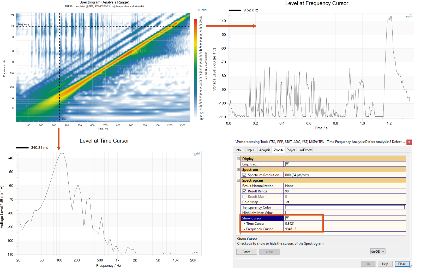
When this checkbox is activated two dashed lines are shown in the spectrogram window. The positions of the cursors correspond to the parameters Time Cursor and Frequency Cursor.

Time Cursor

The Time Cursor specifies the time for the Level at Time Cursor window.

Frequency Cursor

The Frequency Cursor specifies the frequency for the Level at Frequency Cursor window.

Player

Level Settings

Input Level

Shows the relative level of the input signal’s peak value to the maximum value of the playback file in dB. This parameter is not editable.

Normalize Playback Level

When activated the input waveform in playback range will be normalized before playback. This is especially useful if the amplitude of the imported audio signal is very low.

Set Playback Level

Sets the relative level of the input signal’s peak value to the maximum value of the playback file in dB. The maximum value is 0 dB, which is similar to the normalized playback level. The minimum value is -100 dB. This value is only editable, when Normalize Playback Level is deactivated.

Note

When the Input Level is larger than 0 dB, the maximum value of the Set Playback Level is reduced to 0 dB to avoid clipping in the playback.

Playback Settings

Playback Rate

The playback rate of a signal may be changed with this parameter affecting speed and pitch. This is useful if barely audible frequency content or rapid time patterns are selected for playback.

Loop Start

This parameter is connected to the Loop Start Cursor in the Waveform (Time Range) window and to the time value of the cross annotation labeled Lower (shift) in the Spectrogram (Analysis Range) window. It determines the lower limit of the playback time range.

Loop End

This parameter is connected to the Loop End cursor in the Waveform (Time Range) window and to the time value of the cross annotation labeled Upper (shift) in the Spectrogram (Analysis Range) window. It determines the upper limit of the playback time range.

Number of Loops

The number of times the loop is played can be specified using this parameter. If this parameter is empty, the loop will be played back an infinite amount of times. When this parameter is empty and the TFA is used in a batch to playback batch results, the loop will be played back once.

Enable Bandpass Filter

When activated the imported audio signal within the playback range specified in the Input Waveform (Selection) window is band-pass filtered before playback. The filtered signal is then displayed in the Waveform (Time Range) window. When activated and results are available an area is highlighted in the Spectrogram (Analysis Range) window. This area indicates the selected time and frequency range of the filtered playback.

The selected time and frequency range for playback can be changed with the cross annotations in the Spectrogram (Analysis Range) window. The cross annotations can be dragged or clicked. The keyboard shortcuts are:

Upper

Ctrl + Left Mouse Button

Lower

Shift + left mouse button

Play position

Alt + left mouse button

Lower Cutoff Frequency

This parameter is connected to the frequency value of the cross annotation labeled Lower (shift) in the Spectrogram (Analysis Range) window and determines the lower frequency limit for the playback band-pass filter.

Note

This parameter is only visible when the parameter Enable Bandpass Filter is activated.

Upper Cutoff Frequency

This parameter is connected to the frequency value of the cross annotation labeled Upper (shift) in the Spectrogram (Analysis Range) window and determines the upper frequency limit for the playback band-pass filter.

Note

This parameter is only visible when the parameter Enable Bandpass Filter is activated.

Export

Mode

All

In the case of a short wave file the complete imported audio signal is exported without truncation. In case of a long wave file (See Input) the selected time range in the Waveform window is exported.

Selection

In this case, only the selected time range in the Waveform (Time Range) is exported. When the parameter Enable Bandpass Filter is activated, the imported audio signal is filtered before export.

Path

The path and name of the exported audio signal has to be defined here. If the specified wave file already exists the user will be asked if the existing wave file shall be overwritten.

Results

In addition to the spectrogram, the TFA provides various types of results depending on input data and settings.

Waveform

This window shows the imported signal’s waveform. By using the provided cursors, the analysis time range can be adjusted. If a long wave file is imported, this window will show the full wave file content as a bar graph. The bar graph shows peak, bottom and root mean square values of time intervals of the imported wave file. A detailed view of the selected analysis time range is given in the Waveform (Time Range) window.

Waveform (Time Range)

The Waveform (Time Range) window shows the imported audio signal within the selected analysis time range. The cursors can be used to specify the time range for playback. The cursors can be dragged or moved by click. The keyboard shortcuts are:

Loop Start

Shift + Left Mouse Button

Loop End

Ctrl + Left Mouse Button

Play position

Alt + Left Mouse Button

If the parameter Enable Bandpass Filter is enabled, the filtered waveform will be displayed within the selected playback range.

Player Control

The Player Control window gives access to the control of the playback functionality.

Three buttons are available to control playback via your default Windows playback device:

Play

Starts playback of the selected time and frequency range. The start time of the playback is given by the Play Position (Alt) cursors in the Input Waveform (Selection) and the Spectrogram (Analysis Range) windows. When playback is already running this button has no function.

Pause

Pauses the playback. The Play Position (Alt) cursors remain at the time point when the Pause button has been pressed.

Stop

Stops the playback. The Play Position (Alt) cursors are reset to the time position before the start of the playback. The playback can also be stopped by pressing the red cross in the upper toolbar.

The playback volume can be adjusted using the audio device playback level control in the Windows task bar.

Note

If no audio signal is imported, the playback functionality (including the buttons) is not available.

Spectrum

The Spectrum window shows the Fourier transform of the imported time signal. By shifting the cursors, the frequency range of the analysis can be modified.

Note

This window is not available in case of the import of an impulse response. In case of an import of an impulse response the window Transfer Function Magnitude will be available instead of the Spectrum window.

Transfer Function Magnitude

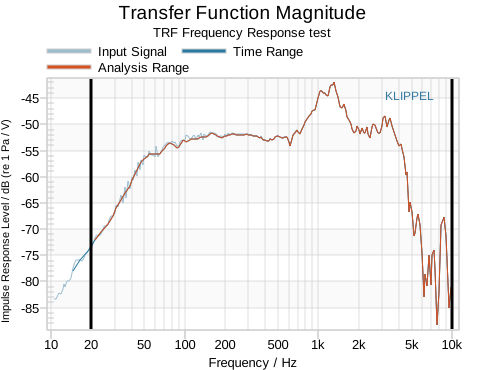
The Transfer Function Magnitude window shows the transfer function that corresponds to an imported impulse response. By shifting the cursors, the frequency range of the analysis can be modified.

Note

This window is only available if an impulse response is imported. If any other audio signal is imported the window Spectrum will be available instead of the Transfer Function Magnitude window.

Energy Time Curve

The Energy Time Curve is showing the signal energy over time. It is normalized to 0 dB. For example, this can be used to determine the reverberation time of a room impulse response.

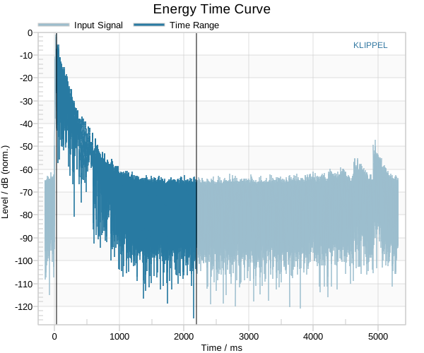
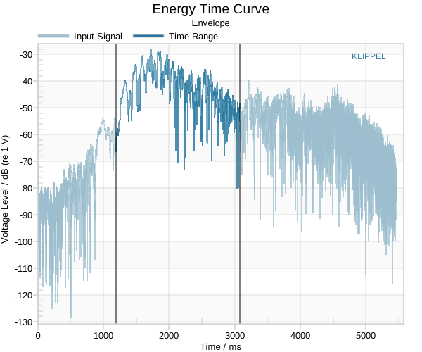
If the imported audio signal is not an impulse response, the curve displayed is the envelope of the the imported signal. If a long wave file (see: Select Input for the definition of a long wave file) is imported the envelope of the selected analysis time range (time range defined in the Waveform window).

Input Signal Characteristics

The TFA is calculating standard signal characteristics (e.g., mean, rms, peak, etc.) of the imported audio signal. This result window is showing these characteristics over time. In addition, the values of the signal characteristics are shown in the Table Results + Settings window.

Note

This window is hidden in case of the import of an impulse response.

Input Crest Factor

The crest factor is the ratio of peak and rms value of a signal. This graph shows the crest factor of the input signal over time.

In addition, the value of the crest factor is shown in the Table Results + Settings window together with the other signal characteristics.

Note

This window is hidden in case of the import of an impulse response.

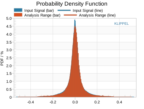
PDF Probability Density Function

The graph shows the probability density function of the imported audio signal.

Note

This window is hidden in case of the import of an impulse response.

Wavelet Waveform

In case the Wavelet transform is used as the analysis method, the time signal of the mother wavelet is shown in this window.

Note

This window is only shown if the Wavelet Transform is selected as Analysis Method.

Wavelet Spectrum

The window shows the frequency response of the mother wavelets, on which the wavelet transform is based.

Note

This window is only shown if the Wavelet Transform is selected as Analysis Method.

Window Function STFT

The graph shows the window function (e.g., von Hann-Window) which is used for the short time Fourier transform.

Note

This window is only shown if the Short Time Fourier Transform is selected as Analysis Method.

Overlapped Windows STFT

For short time Fourier transform the analysis windows are overlapping each other with a specified overlapping factor. The graph shows the position of the windows in time and the resulting overlay.

Note

This window is only shown if the Short Time Fourier Transform is selected as Analysis Method.

Spectrogram

This graph visualizes the signal level over frequency and time. The signal level is represented by a color scale. This is considered the main result window of the TFA module.

Level at Time Cursor

This plot shows the level of the audio signal over frequency for one specific point in time and is a cross section of the spectrogram at the Time Cursor. The value can be defined in the category Display of the Property Page in the section Spectrogram.

Level at Frequency Cursor

This plot displays the level of the audio signal over time for one specific frequency and is a cross section of the spectrogram at the Frequency Cursor. The value can be defined in the category Display of the the Property Page in the section Spectrogram.

3D Plot

This is a 3D representation of the spectrogram. The time resolution of the 3D Plot can be adjusted with the parameter 3D Time Resolution in the category Display in the section 3D Display.

T60(f) Reverberation Times

This window shows the frequency dependent reverberation times as bar graph. Three curves are displayed. The first curve Valid Data shows all the frequencies with a valid reverberation time calculation. The second curve Noise Corrupted shows the frequency bins which are noise corrupted resulting in an invalid reverberation time calculation. The third curve Impulse Response Too Short shows for which frequencies the impulse response is too short, indicating that a longer measurement is needed for particular frequencies. The error Impulse Response Too Short is thrown when the energy of the frequency bin does not reach a minimum decay of 40 dB.

The dotted horizontal line shows the global reverberation time (frequency independent). Additionally, the value is shown in the subtitle of the window.

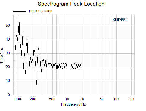
Spectrogram Peak Location

The Peak Location curve shows, at which point of time the maximum level of any frequency band is reached. The results may be normalized to this curve if the option To Fundamental of the parameter Result Normalization is selected (see Result Normalization). This window is only available if no impulse response was imported.

Group Delay

In signal processing, group delay is the time delay of the amplitude envelopes of the various frequency components of a signal through a device under test, and is a function of frequency for each component. Delays caused by resonators (e.g., vented boxes) can be evaluated with the group delay. This window is only available when an impulse response was imported and if the Wavelet Transform is selected as Analysis Method.

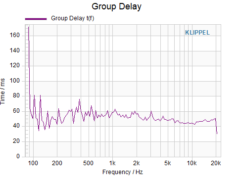
Table Results + Settings

The window summarizes important settings and results, such as:

• Properties of the input data (e.g., length, sample rate, impulse response import)

• Calculated signal characteristics

• Settings of the TFA Analysis Method

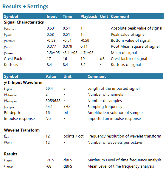
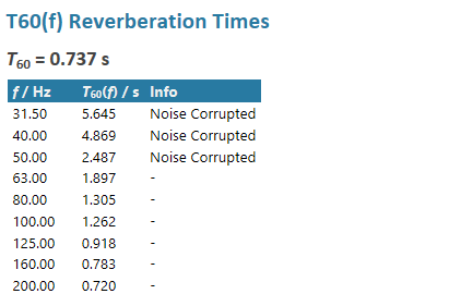
Table T60(f) Reverberation Times

This table shows all the calculated reverberation times and errors for each frequency bin.

Supported Modules for Im/Export

The TFA module can import time domain signals from any other module in the KLIPPEL Analyzer System. However, the generic import requires that the windows to import data from has the keywords “Waveform” or “Impulse Response” in its title. Otherwise, you can always use clipboard import for importing raw time series data.