LSIM – Linear Simulation#
LSIM - Getting Started Guide#
This document gives a quick overview of the main features of linear simulation (LSIM) and its usage.
Setup Driver and System properties#
The linear simulation module (LSIM) is a tool to investigate the linear behaviour of common active and passive loudspeaker systems. To start the simulation, all required parameters have to be entered.
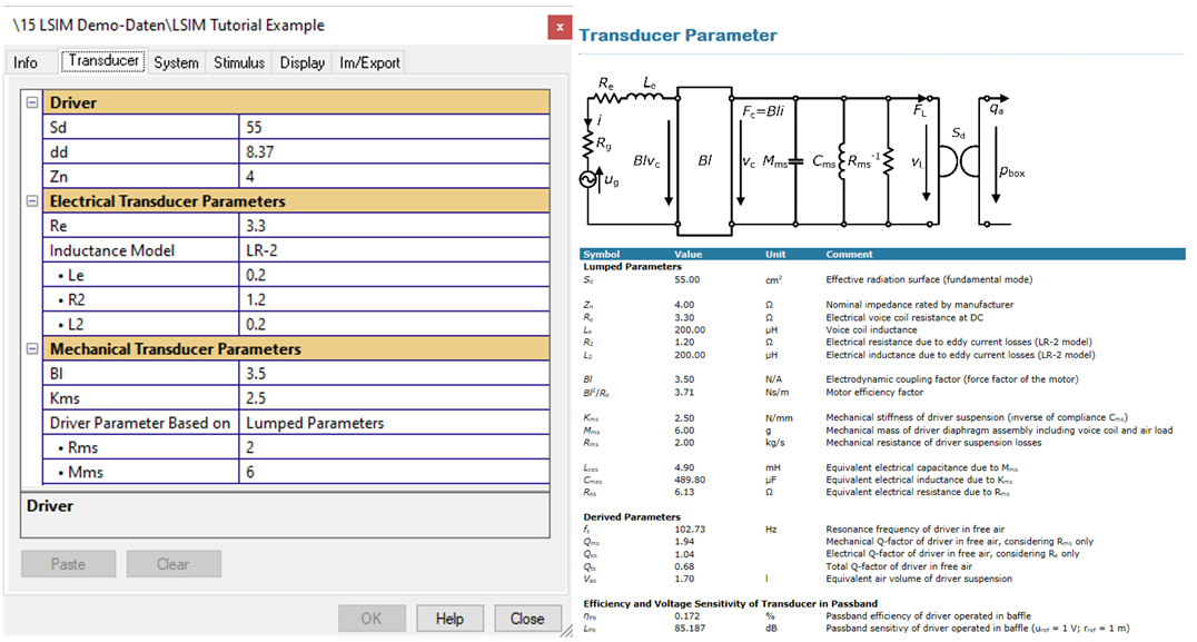
View the property page Transducer to enter transducer-related parameters.
Select one of the inductance models to specify the voice coil inductance
The select list Driver Parameter based on provides the option to enter a desired fs and Qms instead of the common Mms and Rms for the current transducer.
All entered and derivable transducer parameters (e.g., fc, Cab) are immediately updated and shown in the window Table Transducer Parameters after changing any parameter.
Note
If an LPM measurement is available for a current transducer, all required transducer parameters can be entered by using the function Import from Clipboard.
The System property page contains parameters for describing the whole active loudspeaker system. The first section Equalization is described in the next section.
Amplifier - Rg: Define amplifier and cable resistance
Enclosure: This section contains parameters to describe the enclosure in which the transducer is mounted. Select one of the proposed system types and specify its properties.
All entered and derived system parameters (e.g. fc, Kmt) are immediately updated and shown in the window Table System Parameters.
After entering all relevant data run  the operation.
Setup Equalization#
To simulate linear speaker states, average sensitivity and average efficiency with a system response close to the target application, you can use the equalization tool. Two options are available:
- Input response
Enter a desired target transfer behaviour by entering a frequency axis with corresponding values. Based on the entered data, a target transfer function is approximated. The corresponding equalizer transfer function will be calculated automatically.
- HP-Filter Alignment
Specify a high pass filter as target behaviour. Typical filter types like Bessel, Chebychev and Butterworth are available.
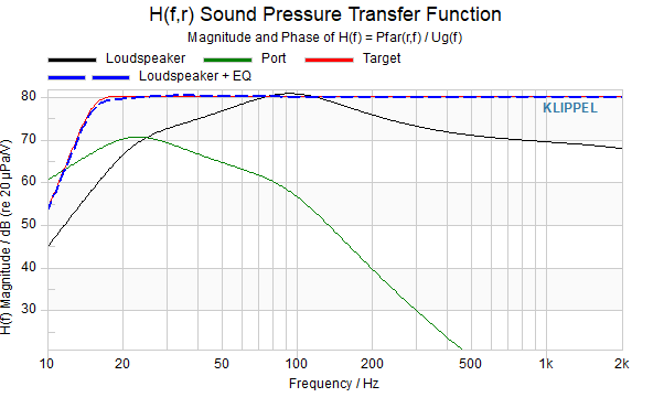
If any equalization is chosen, the window H(f) Equalizer appears which contains the equalizer transfer function. Additionally to this two curves will be available in the window H(f,r) Sound Pressure (by right-click in the window and selecting Show all Curves). The blue curve is the resulting total sound pressure of the system with equalization. The red curve is the desired target transfer behaviour. For the correct calculated equalizer function, both curves should be the same.
Pay attention: If the checkbox compensate inductance is switched off, the resulting total sound pressure and target sound pressure may differ.
Setup external Stimulus#
The LSIM features the option to investigate the linear behaviour of a loudspeaker system for a certain stimulus. If you want to use your own stimulus, follow these instructions:
Type of Input Signal: Select External Spectrum
Bandwidth: Check if the frequency axis of your entered spectrum is constant or relative (e.g., logarithmical spaced)
Relative Spectrum: Enter your desired spectrum (If you want to investigate the behaviour for a certain .wav file, view section Use TFA to Generate a Spectrum)
Crest Factor: Enter the crest factor of your stimulus to estimate peak values of voltage, current and displacement. The Delta CF parameter defines the difference of crest factor (in dB) between voltage and displacement.
Filter: This section provides the option to add a high- and low-pass filter to the stimulus. For reducing the bandwidth of the stimulus to a certain area, you can use the filter option Sharp Transition.
Target: Choose a target value SPLmax or Umax which will be reached for the entered relative stimulus. This is important to derive an absolute spectrum and absolute values from the entered relative spectrum.
The entered stimulus will be transformed internally into a third-octave-spaced spectrum. All results are available after running the operation. Single values are displayed in the window System States.
Note
The chosen stimulus has no influence on the transfer functions. All stimulus-related windows are labelled with Spectrum or stimulus. If you want to investigate the influence of the stimulus on certain states view the window State Spectrum. You can select the state of interest on the property page Display State spectrum signal.
Use TFA to Generate a Spectrum#
If you want to use a .wav file for defining a stimulus the easiest way is to use the TFA – Time Frequency Analysis-module.
Create a TFA operation
 (New Operation) -> Post-Processing Tools -> TFA
Time-Frequency Analysis.
(New Operation) -> Post-Processing Tools -> TFA
Time-Frequency Analysis.Open to the property page
 and open the Input page and Select input -> File, select
the desired .wav-file and Import
and open the Input page and Select input -> File, select
the desired .wav-file and ImportYou can define the time range which is used for Fourier transformation in Waveform(t).
Copy the curve from the window Spectrum (f). (Right-click on the curve -> copy curve)
Open the LSIM-operation and open the property page -> Stimulus. Choose relative for the parameter Bandwidth).
Paste the TFA’s spectrum from the clipboard to relative Spectrum.
LSIM – Tutorial#
Overview#
The LSIM module performs numerical simulations of active electroacoustic systems comprising a prefilter, equalizer, amplifier and electrodynamical transducer mounted in a common enclosure system. The LSIM employs a linear lumped parameter model to derive the system parameters of the passive loudspeaker system and to simulate its transfer behaviour. Based on typical audio program material, average values for efficiency, sensitivity and RMS values of transducer states are estimated. This is useful for optimizing the electroacoustic system in terms of efficiency or maximum SPL.
What is the goal of this tutorial?#
Familiarize with the LSIM module.
Overview of basic features of the LSIM
Detailed information about the linear transducer model, a detailed description of the result windows and the configuration of the property pages can be found in the chapter LSIM Reference.
Using LSIM for active loudspeaker design#
This tutorial uses a practical example. The task is to use the LSIM for designing a two-way closed-box loudspeaker. We define the following design targets:
The desired SPL output is 95 dB in a 1 m distance in a half-room.
The volume of the box is limited to 1 l due to design choices.
A 4” transducer with a maximum specified displacement of xmax = 5 mm shall be used.
Crossover frequency to the tweeter fxo=5 kHz
The following critical single values should be determined for typical program material with respect to these design targets:
Power and voltage consumption (required for selecting a fitting amplifier)
Efficiency and Voltage Sensitivity
Peak voice coil displacement
LSIM parameters#
Example data used in this manual is stored in the Web Example Database. If not downloaded already, get it from the latest R&D release <https://www.klippel.de/go/current-rnd-release> and open the web-based database.
See also
View Results for general information on how to download this database, open and view results in dB-Lab.
Open folder \Simulation, Auralization (LSIM, SIM, SIM-AUR, DIF-AUR, ALS) \Linear Simulation (LSIM).
Open the object  LSIM and double click the operation LSIM Xpeak Typical IEC Stimulus
(Closed Box). Clicking on
LSIM and double click the operation LSIM Xpeak Typical IEC Stimulus
(Closed Box). Clicking on  opens the property page. Here, any parameter can be entered and
adjusted. For the current task, only the sections Transducer, System and Stimulus are
relevant.
opens the property page. Here, any parameter can be entered and
adjusted. For the current task, only the sections Transducer, System and Stimulus are
relevant.
Linear Transducer Parameters#
Data of a small midrange speaker was imported from an LPM operation.
System parameters#
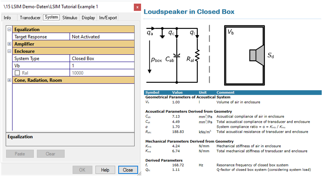
The closed box loudspeaker is specified with a volume of 1 l. In the first step, no equalization is applied to the system.
For simplification, no amplifier output resistance Rg, leakage losses Ral and post-filter are selected. The window Table System Parameters shows the headline Loudspeaker in Closed Box indicating the selected enclosure system. The picture below shows the corresponding equivalent circuit. The table below contains all derived enclosure parameters based on the entered closed-box parameters.
Stimulus Parameters#
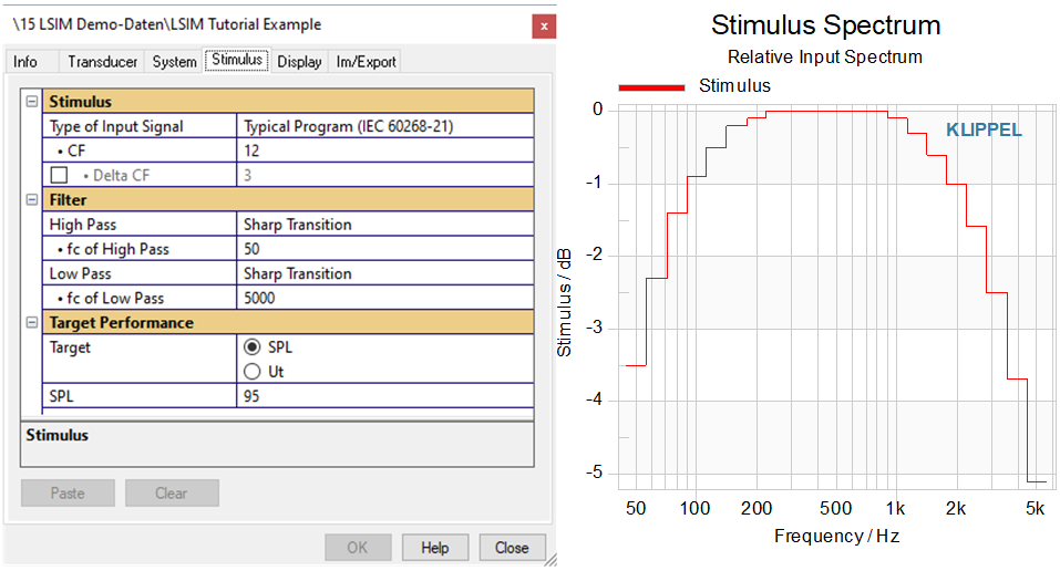
The stimulus used for calculating the transducer and system states is specified on the property page Stimulus. The spectrum defined in IEC 60268-21 represents common broadband music stimuli. A typical crest factor is 12 dB. For the specified small speaker, the frequency band from 50 Hz (SPL output is negligible below) to 5 kHz (crossover frequency) shall be considered. The desired SPL of 95 dB is specified in Target SPL. The window stimulus spectrum shows the relative stimulus spectrum.
A detailed list of all parameters and options is available in the section reference.
Viewing Results#
The first results are available immediately after entering all data on the property page. This affects all parameters shown in the windows Table Transducer Parameters (red) and Table System Parameters (green). Activate the desired windows in the box at the bottom left side (purple) of dB-Lab.
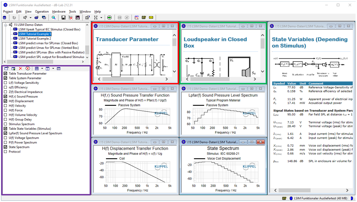
Start the simulation by pressing the button  Run or using the shortcut Ctrl + R.
Note
For each transfer function, a phase curve is available via the curve settings (Press the right mouse button on the window, then choose Customize…. In the appearing window, choose the desired curves at the tab subset). Other variations of the transfer functions are available in the same way.
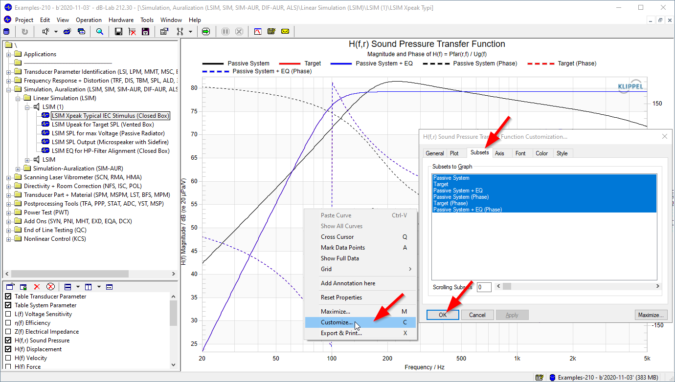
Analyzing Results#
The single values listed in table Table State Variables (Stimulus) provide the most important information considering the simulated music reproduction:
For generating 95 dB SPL output using the desired IEC signal, the amplifier has to provide about 11 W. The peak voltage for an estimated crest factor of 12 is approx. 28 V.
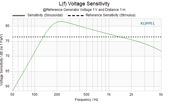
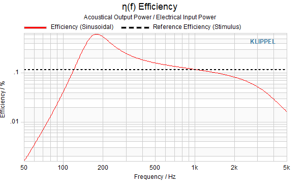
The resulting effective (reference) efficiency is approx. 0.16 % for the selected stimulus. The effective (reference) voltage sensitivity is 78 dB.
For the specified stimulus, a peak displacement of approx. 2.86 mm is expected.
These values are the basis for defining the amplifier and transducer requirements. Checking the limits defined in the task above reveal that the desired SPL is achievable without exceeding the transducer’s maximum displacement.
Viewing the curves efficiency and voltage sensitivity versus frequency is useful to understand the limitations of the passive loudspeaker system. The efficiency at lower frequencies decreases rapidly, so pushing frequencies to very low frequencies will be inefficient. Pay attention: Efficiency and voltage sensitivity is not equal. Efficiency shows the ratio between incoming and outgoing power in percent. Voltage sensitivity shows the SPL output at a 1 m distance with a terminal voltage of 1 V.
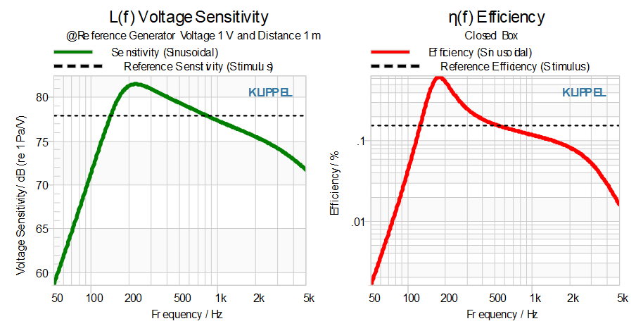
Adding Equalization#
As the sound pressure transfer function (see chart below) shows, the frequency response is not equalized and the cutoff frequency is very high (~170 Hz).
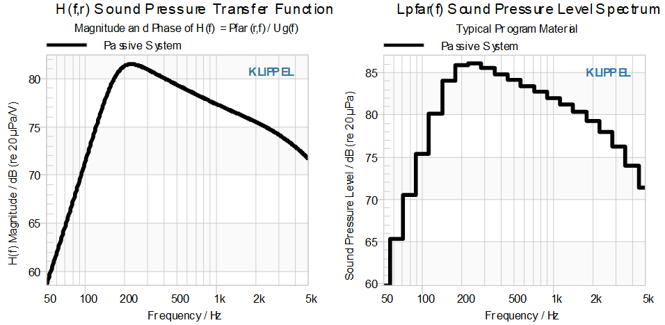
This section explains how to reduce the active system’s cut-off frequency and how to apply equalization at higher frequencies.
Finding a good compromise for the optimal target high-pass characteristic is crucial for optimum performance: Setting the cut-off frequency too low will result in an inefficient system prone to extreme voltage requirements. Setting the cut-off frequency too high leads to a lack of bass and wasted potential. For the first simulation we define the following target response:
Cut-off frequency: 60 Hz
Filter type: 6th order Chebyshev filter
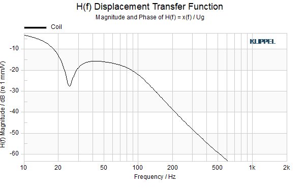
A 6th order filter is used to avoid wasting voltage and displacement below the cut-off frequency where the voltage sensitivity drops significantly (Compare H(f,r) Sound Pressure and H(f) Displacement). See the sound pressure transfer function and spectrum which shows the impact of the alignment filter on the sound pressure.
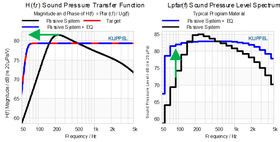
Applying this alignment filter results in a peak voltage of approx. 47 V and an electrical power of almost 34 W to achieve the desired 95 dB SPL output. The required peak displacement is 6.6 mm now. These values have increased dramatically compared to the passive system. This is caused by the excessive bass boost defined by the target alignment. As can be seen in the chart below, the alignment is boosting low frequencies up to 15 dB. In the State Variables window, the effective voltage boost LEQ for the selected stimulus is displayed (in this case the boost is 5.5 dB).
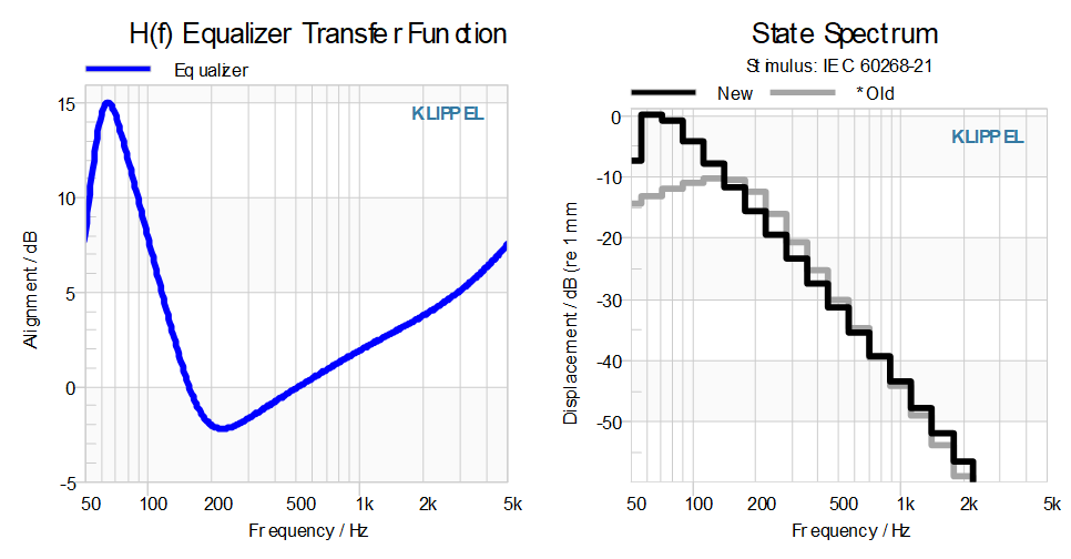
As the estimated displacement exceeds the transducer specification and the electrical power will heat up the voice coil too much (typical thermal resistance of this transducer type is 3…5 K/W) reducing efficiency, the initially used cut-off frequency should be increased.
For the next simulation we use the following target alignment:
Cut-off frequency: 75 Hz
Filter type: 6th order Chebyshev filter
Now the peak voice coil displacement is below the limit (xc,peak = 4.7 mm), the electrical power for this stimulus is 20 W and the peak voltage is 38 V. If the amplifier can deliver this voltage, the chosen target alignment is reasonable. If a weaker amplifier is used, the cut-off frequency has to be increased or the design targets to be relaxed.
Comparing the reference efficiency and reference voltage sensitivity between the passive system and the equalized system reveals that the bass enhancement results in a speaker with a linear frequency response and much better low-frequency response at the cost of lower efficiency:
LR, old = 77.9 dB; ηR, old = 0.16 %;
LR, new = 75.4 dB; ηR, new = 0.09 %;
LSIM – Reference#
Overview#
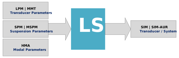
The Linear Simulation (LSIM) module performs a numerical simulation of an active loudspeaker system containing a bandpass filter, equalization filter, amplifier, and an electro-dynamical driver mounted in a common enclosure and a postfilter. A lumped parameter model is used to describe the transfer behaviour of the whole system in the linear domain. The input data of this routine are parameters of a real or virtual driver, geometrical parameters of an enclosure and stimulus properties. To investigate a real transducer, parameters from an LPM-measurement can be imported via clipboard. Further investigations about nonlinear behaviour are possible in the SIM and SIM-AUR module. Use the clipboard-export function to transfer parameters easily.
Theory#
The theory of the LSIM module is highly related to the papers Green Speaker Design, Part 1 and Part 2. The LSIM module describes the linear behaviour of a simplified active loudspeaker system. Nonlinear behaviour such as varying force factor Bl or mechanical stiffness Kms versus voice coil position will be neglected.
(Green Speaker Design Part 1, Green Speaker Design Part 2)
Stimulus based Processing#
Simulating the behaviour of an active loudspeaker system for a certain stimulus spectrum provides very useful information for optimizing the system, such as average efficiency and sensitivity and estimated peak displacement. The stimulus-based processing is implemented as displayed in the signal flow chart below.
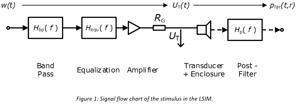
A relative third octave spaced spectrum w(f) of the desired broadband signal (e.g. music) has to be defined on the LSIM’s property page. Several spectra, such as the spectrum of the stimulus after the equalizer filter is calculated and displayed. From these spectra, statistical single values like Lpfar and UT,rms as well as UT,peak and xC,peak are derived. More detailed information about the calculation of these state variables is available in the papers green Speaker Design part 1 and 2 by Wolfgang Klippel.
Lumped Parameter Model#
The simulation is based on a lumped parameter model of an electro-dynamical transducer mounted in an enclosure. Based on this, the LSIM calculates state variables and transfer functions.
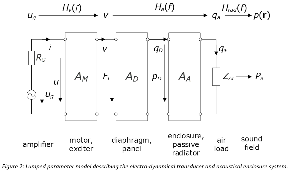
Voice Coil Inductance#
The LSIM supports several inductance models which will lead to slightly different simulation results. The simplest approach consists of a series connection of a resistor Re and an ideal inductance Le. This model is only applicable for transducers with a very small inductance (micro-speakers) because eddy currents in the iron parts of the transducer’s motor are neglected. The following inductance models considering these losses are available:
LR-2 Model#
The LR=2 model adds an inductor L2 shunted by the resistance R2 to the single inductance Le. The impedance of the LR-2 model is
with omega = 2πf. This model usually works well for frequencies up to 40 times fs, where fs is the resonance frequency of the driver.
LR-3 Model#
This model is an expansion of the LR=2 Model with another inductance L3 and resistance R3. The impedance of the LR-3 model is given by
LEACH Model#
If losses in the transducer’s iron parts are not negligible, the phase of the inductor’s impedance is smaller than 90°. The LEACH model considers this by only using two parameters:
WRIGHT Model#
The relation between the real and imaginary parts of the LEACH model is fixed leading to a constant, frequency-independent phase. The WRIGHT model gives more degrees of freedom as the real and imaginary parts of the impedance are independent:
Enclosure#
The LSIM module supports the most common enclosure types. The following section provides a detailed description including all parameters.
Driver in Baffle#
The baffle simulation is a useful tool to focus on the transducer. For this model, the driver is assumed to be mounted in an infinite baffle, so no acoustical shortcut is present.
Closed Box#
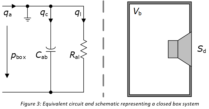
The closed box system is the simplest enclosure system. Therefore, only the specification of a box volume is needed. According to this, the compliance of the air in the box is calculated. Losses due to air leakage can be simulated by entering a value for Ral. For the ideal box without any air leakage, \(R_\text{al}\to \infty\).
Vented Box#
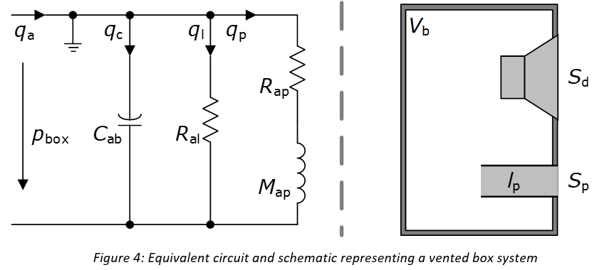
The vented box system is mainly characterized by the box volume and the geometry of the vent, which shape can be a tube or a slit. The vent acts as a Helmholtz resonator which resonance depends on box volume and air mass in the port. The acoustical parameters Rap and Map can be entered directly or calculated based on the vent’s geometry or based on its resonance frequency and Q-factor.
Passive Radiator System#
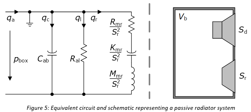
An enclosure system with a passive radiator has a relatively similar behaviour to a vented box system. However, the passive radiator’s resonance frequency defined by its mass and stiffness will produce a dip in the sound pressure response which is usually far below the cut-off frequency. The passive radiator is characterized by its effective radiating surface Sr, the mass of the moving parts Mmr, mechanical losses Rmr and the suspension stiffness Kmr.
Bandpass System#
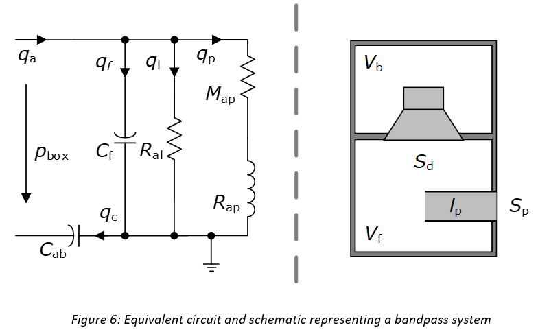
The bandpass system is a special kind of vented box system using a transducer mounted between two volumes. The front volume contains a vent for sound radiation. This design is used to generate high amplitudes in a limited frequency range.
Bandpass Filter#
The LSIM module provides several low- and high-pass filters which is for instance required if the transducer is used in a multi-way system. These filters are only applied to the stimulus spectrum and are not visible in the transfer functions of the passive loudspeaker. The filter order and cutoff frequency can be adjusted.
The filter option sharp Transition represents a so-called ideal filter. This theoretical filter has an infinite slope. The aim of this is to limit the frequency band of the stimulus to the desired bandwidth.
Equalization#
For simulating the states of an active loudspeaker system for a certain stimulus (such as typical program material) as used in the final application, an equalizer transfer function has usually to be specified. This can be done by either entering a target transfer function or defining a high-pass filter which represents the target transfer function.
Target Response: A target transfer function P(f)/U(f) can be defined by a frequency-level matrix. The level has to be entered as absolute level in dB. The frequency-resolution of the entered matrix is interpolated to the LSIM’s internal resolution.
The equalizer transfer-function is calculated by dividing the specified target transfer behavior by the simulated transfer function of the passive loudspeaker system.
High-Pass Alignment: System alignment filters are usually used for lowering the cut-off frequency of the speaker system (bass boost). Instead of using generic parametric equalizers, the LSIM automatically calculates Biquad filters based on the user’s requirements. The following high-pass filters are available:
2nd Order Filter
4th Order Butterworth/ Chebyshev/Bessel
6th Order Butterworth/ Chebyshev/Bessel
If the High-Pass Filter Alignment is selected, the equalizer transfer-function is calculated using different approaches according to the specified loudspeaker enclosure system.
For all enclosure types except Bandpass systems, the alignment filter is automatically calculated based on the lumped parameters of the passive speaker system and the desired target alignment. The alignment filter consists of one (2nd order target function), two (4th order target) or three (6th order target) Biquad filters.
For band-pass systems, HEQ(f) is calculated by dividing the specified target high-pass filter by the transfer function of the passive loudspeaker system.
Note
The checkbox Compensate Inductance adds a linear filter to compensate the decrease of sound pressure output at higher frequencies. Note that if the inductance is not compensated, deviations between target and active system transfer behaviour are expected as the Biquad filters contain no inductance modelling. This structure is also used in the Klippel Controlled Sound (KCS).
Post-Filter#
With a post-filter, the characteristics of a room or other acoustical components can be added to the LSIM model. The LSIM provides an interface for complex transfer functions in the format of magnitude and phase.
Property Pages#
The following section contains a description of all input parameters of the LSIM module. The section is structured analogously to the property pages.
Transducer#
The property page transducer comprises all parameters related to the electrodynamical transducer. The visibility of the parameters for the voice coil modelling is adjusted according to the chosen model. Switching between lumped and derived parameters for the base of the parameter calculation allows the user to enter the resonance frequency fS and the mechanical Q-factor Qms of the transducer (under free air conditions). According to this, Rms and Mms will be calculated.
Transducer Parameters#
- \(S_{d}\)
- Unit: \(\text{cm}^{2}\)Effective radiation surface
- \(d_{d}\)
- Unit: \(\text{cm}\)Diameter of round effective radiation surface
- \(Z_{n}\)
- Unit: \(\Omega\)Nominal impedance rated by the manufacturer
- \(R_{e}\)
- Unit: \(\Omega\)Electrical voice-coil resistance at DC
- \(L_{e}\)
- Unit: \(\text{mH}\)Voice coil inductance
- \(R_{2}\)
- Unit: \(\Omega\)Electric resistance due to eddy current losses
- \(L_{2}\)
- Unit: \(\text{mH}\)Electrical inductance due to eddy current losses
- \(R_{3}\)
- Unit: \(\Omega\)Electric resistance due to eddy current losses
- \(L_{3}\)
- Unit: \(\Omega\)Electric inductance due to eddy current losses
- \(K\)
- Unit: \(\Omega\)Factor in LEACH model
- \(n\)
- Exponent in LEACH model
- \(K_{\text{rm}}\)
- Unit: \(\Omega\)Factor of real part in WRIGHT model
- \(E_{\text{rm}}\)
- Exponent of real part in WRIGHT model
- \(K_{\text{xm}}\)
- Unit: \(\Omega\)Factor of imaginary part in WRIGHT model
- \(E_{\text{xm}}\)
- Exponent of imaginary part in WRIGHT model
- \(\text{Bl}\)
- Unit: \(\text{N/A}\)Effective instantaneous electrodynamic coupling factor (force factor of the motor) defined by the integral of the magnetic flux density B over the voice coil length l
- \(K_{\text{ms}}\)
- Unit: \(\text{N/mm}\)Mechanical stiffness of driver suspension (inverse of compliance Cms)
- \(R_{\text{ms}}\)
- Unit: \(\text{kg/s}\)Mechanical resistance of driver suspension losses
- \(M_{\text{ms}}\)
- Unit: \(\text{g}\)Mechanical mass of driver diaphragm assembly including voice coil and air load
- \(f_{s}\)
- Unit: \(\text{Hz}\)Transducer resonance frequency in free air
- \(Q_{\text{ts}}\)
- Mechanical Q-factor of driver in free air, considering mechanical system only
System#
The property page system is divided into 4 sections. Each section represents one part of the active loudspeaker system.
Equalization#
The equalizer transfer function in the LSIM module is calculated automatically to reach the entered target transfer behaviour. Therefore, two different approaches are provided:
Not activated (default value if no equalization is chosen)
Input response provides the option to enter a frequency shape or spectrum of the desired transfer behaviour.
In case of HP-Filter Alignment the target transfer behaviour is defined by one of the common high pass filter structures. Therefore, only a target cutoff frequency, and in some cases, a q-factor or constant has to be defined. The following high-pass filter structures are available:
2nd Order Filter
Bessel Filter (4th and 6th order)
Chebyshev Filter (4th and 6th order)
Butterworth Filter (4th and 6th order)
For both cases, the equalizer function is calculated and displayed automatically.
- \(f_{0}\)
- Unit: \(\text{Hz}\)Target Cutoff Frequency
- \(K\)
- Chebyshev Constant (only available for Chebyshev Filters)
- \(Q\)
- Target Q Factor (only available for 2nd Order Filter)
Amplifier#
The LSIM module provides the option to enter the output resistance of the amplifier including cables. With this value, it is possible to get information about the open voltage that must be provided by the amplifier.
- \(R_{g}\)
- Unit: \(\Omega\)Output-resistance of amplifier output including cables
Enclosure#
This section of the property page, related to the enclosure, will be adapted based on the selected enclosure. Every parameter that is not necessary for the chosen system will be hidden by the system. Derivable parameters are calculated automatically and displayed in the window System Parameter. The port can be specified by its geometry, derived parameters or lumped parameters.
Geometrical parameters:#
- \(V_{b}\)
- Unit: \(\text{l}\)Volume of air in the enclosure
- \(S_{p}\)
- Unit: \(\text{cm}^{2}\)Surface area of the port
- \(d_{p}\)
- Unit: \(\text{cm}\)Diameter of port
- \(l_{p}\)
- Unit: \(\text{cm}\)Length of port
- \(w_{p}\)
- Unit: \(\text{cm}\)Width of the surface area of the port
- \(h_{p}\)
- Unit: \(\text{cm}\)Height of surface area of the port
- \(S_{r}\)
- Unit: \(\text{cm}^{2}\)Effective projected surface area of passive radiator diaphragm
- \(d_{r}\)
- Unit: \(\text{cm}\)Diameter of the round effective projected surface area of passive radiator diaphragm
- \(V_{f}\)
- Unit: \(\text{l}\)Volume of air in front enclosure
Lumped parameters:#
- \(R_{\text{al}}\)
- Unit: \(\text{kNs/m}^{5}\)Acoustic resistance of losses due to leakage
- \(R_{\text{ap}}\)
- Unit: \(\text{kNs/m}^{3}\)Acoustic mass of port including air load
- \(M_{\text{ap}}\)
- Unit: \(\text{kg/m}^{4}\)Acoustic resistance of port losses
- \(M_{\text{mr}}\)
- Unit: \(\text{g}\)Mechanical mass of passive radiator diaphragm including voice coil and air load
- \(K_{\text{mr}}\)
- Unit: \(\text{N/mm}\)Mechanical stiffness of passive radiator suspension (inverse of compliance Cmr)
- \(R_{\text{mr}}\)
- Unit: \(\text{kg/s}\)Mechanical resistance of passive radiator suspension losses
Derived parameters:#
- \(Q_{l}\)
- Q-factor of acoustic system at fb considering leakage losses
- \(f_{b}\)
- Unit: \(\text{Hz}\)Resonance frequency of enclosure-port system
- \(Q_{p}\)
- Q-factor considering port losses
- \(f_{f}\)
- Unit: \(\text{Hz}\)Resonance frequency of the enclosure-port system
Cone, Radiation, Room#
This section contains parameters to define the environment for the simulation. With the radiation model, it is possible to switch between half-space and full space. The distance to the radiation point can be defined with the parameter Distance. With the optional Post Filter, a complex transfer function in the format of magnitude and phase can be used to describe additional acoustical influences.
Stimulus#
The LSIM module provides a separate property page to specify a relative spectrum at the input of the system. This signal is completely independent of the signal used to calculate the transfer functions. The signal for the calculation of the transfer functions is defined internally as a frequency sweep from 1 Hz to 100 kHz with 2,000 logarithmically spaced points.
The LSIM provides 3 options for specifying an input stimulus (view the table below). Additionally, a high pass and low pass filter can be used to simulate, for example, a crossover. The parameter CF, Crest Factor, is the ratio between peak and RMS values of the signal in the time domain. This is used to estimate peak values. The LSIM uses one single crest factor for all signals (current, voltage, displacement etc.). However, the crest factor of the current and voltage signal is usually higher than the crest factor of the displacement and velocity signals. Therefore, a parameter ∆CF which represents the difference between the voltage’s and the displacement’s crest factor is introduced.
Pink Noise: Each frequency band contains the same amount of power.
Typical program material according to IEC 60268-21: Standardized spectrum, which represents typical spectra of common music.
External Spectrum: Option to enter a certain relative spectrum of a stimulus by user input of a frequency and corresponding level matrix. This option must be handled with care. Using a strange spectrum may lead to misleading results. The frequency axis of the external spectrum has to be specified as relative (logarithmic) or linear spaced.
The entered and specified input spectrum will be automatically transformed into a third octave-spaced spectrum. This relative spectrum will be converted to absolute values using a desired SPLmax or Umax. Umax can be entered as the maximal RMS voltage or the maximal peak voltage at the transducer terminals.
- \(f_{\text{cHP}}\)
- Unit: \(\text{Hz}\)Cutoff frequency of the high pass filter
- \(m_{\text{HP}}\)
- Unit: \(\text{dB}\)Slope of high pass filter
- \(f_{\text{cLP}}\)
- Unit: \(\text{Hz}\)Cutoff frequency of the Low pass filter
- \(m_{\text{LP}}\)
- Unit: \(\text{dB}\)Slope of low pass filter
- \(\text{CF}\)
- Unit: \(\text{dB}\)Crest factor
- \(\mathrm{\Delta}\text{CF}\)
- Unit: \(\text{dB}\)Difference between crest factor for voltage and current signal and crest factor for displacement signal
Display#
This property page is divided into three sections:
General: Here it is possible to adjust the displayed frequency range.
Transfer Function: The parameter Scaling Y-Axis defines if the y- axis is absolute (linear) scaled or uses the relative representation in dB.
Spectrum: The parameter State Spectrum Signal defines the spectrum which is shown in the window State Spectrum. The parameter Scaling Y-Axis has the same function for the spectra as described above for the transfer functions.
Changes on this page will not affect any results.
Results Windows#
The following section provides a detailed description of every result window available in the LSIM module.
Transducer Parameter#
This window contains a picture of the equivalent circuit representing the electro-mechanical part of the transducer and a table with all available transducer parameters including the well-known Thiele-Small parameters. This window is updated after each change in the property page. All derivable parameters will be calculated and displayed automatically. Only the passband sensitivity and efficiency are excluded from this.
- \(S_{d}\)
- Unit: \(\text{cm}^{2}\)Effective radiation surface (fundamental mode)
- \(d_{d}\)
- Unit: \(\text{cm}\)Diameter of round effective radiation surface
- \(Z_{n}\)
- Unit: \(\Omega\)Nominal impedance rated by manufacturer
- \(R_{e}\)
- Unit: \(\Omega\)Electrical voice coil resistance at DC
- \(L_{e}\)
- Unit: \(\text{mH}\)Voice coil inductance
- \(R_{2}\)
- Unit: \(\Omega\)Electric resistance due to eddy current losses (LR-2 model)
- \(L_{2}\)
- Unit: \(\text{mH}\)Electrical inductance due to eddy current losses (LR-2 model)
- \(R_{3}\)
- Unit: \(\Omega\)Electric resistance due to eddy current losses (LR-3 model)
- \(L_{3}\)
- Unit: \(\text{mH}\)Electrical inductance due to eddy current losses (LR-3 model)
- \(K\)
- Unit: \(\Omega\)Factor in LEACH model
- \(n\)
- Exponent in LEACH model
- \(K_{\text{rm}}\)
- Unit: \(\Omega\)Factor of real part in WRIGHT model
- \(E_{\text{rm}}\)
- Exponent of real part in WRIGHT model
- \(K_{\text{xm}}\)
- Unit: \(\Omega\)Factor of imaginary part in WRIGHT model
- \(E_{\text{xm}}\)
- Exponent of imaginary part in WRIGHT model
- \(\text{Bl}\)
- Unit: \(\text{N/A}\)Effective instantaneous electrodynamic coupling factor (force factor of the motor) defined by the integral of the magnetic flux density B over the voice coil length l
- \(K_{\text{ms}}\)
- Unit: \(\text{N/mm}\)Mechanical stiffness of driver suspension (inverse of compliance Cms)
- \(R_{\text{ms}}\)
- Unit: \(\text{kg/s}\)Mechanical resistance of driver suspension losses
- \(M_{\text{ms}}\)
- Unit: \(\text{g}\)Mechanical mass of driver diaphragm assembly including voice coil and air load
- \(f_{s}\)
- Unit: \(\text{Hz}\)Transducer resonance frequency in free air
- \(Q_{\text{ts}}\)
- Mechanical Q-factor of driver in free air
- \(Q_{\text{ms}}\)
- Mechanical Q-factor of driver in free air, considering Rms only
- \(Q_{\text{es}}\)
- Electrical Q-factor of driver in free air, considering Re only
- \(V_{\text{as}}\)
- Unit: \(\text{l}\)Equivalent air volume of driver suspension
- \(\eta_{\text{Pb}}\)
- Unit: :math:` %`Passband efficiency of driver operated in baffle
- \(L_{\text{Pb}}\)
- Unit: \(\text{dB}\)Passband sensitivity of driver operated in baffle with reference voltage uref = 1 V and reference distance rref defined in ppg. System
System Parameters#
The window System Parameter presents the equivalent circuit and a schematic picture representing the enclosure system. This picture varies according to the entered data. The table below contains every parameter related to the enclosure system. This table is divided into four sections. The first section contains geometrical measures like volume. The second section contains acoustical parameters, which are also used for the description of the equivalent circuit. The third section contains derived parameters like resonance frequency and Q-factors. All of these parameters are calculated and updated automatically after changing any input data.
Geometrical parameters:#
- \(V_{b}\)
- Unit: \(\text{l}\)Volume of air in enclosure
- \(S_{p}\)
- Unit: \(\text{cm}^{2}\)Surface area of port
- \(d_{p}\)
- Unit: \(\text{cm}\)Diameter of port
- \(l_{p}\)
- Unit: \(\text{cm}\)Length of port
- \(w_{p}\)
- Unit: \(\text{cm}\)Width of surface area of port
- \(h_{p}\)
- Unit: \(\text{cm}\)Height of surface area of port
- \(S_{r}\)
- Unit: \(\text{cm}^{2}\)Effective projected surface area of passive radiator diaphragm
- \(d_{r}\)
- Unit: \(\text{cm}\)Diameter of round effective projected surface area of passive radiator diaphragm
- \(V_{f}\)
- Unit: \(\text{l}\)Volume of air in front enclosure
Lumped parameters:#
- \(C_{\text{ab}}\)
- Unit: \(\text{m}^{3}\text{/Pa}\)Acoustical compliance of air in enclosure
- \(K_{\text{mb}}\)
- Unit: \(\text{N/mm}\)Mechanical stiffness of air in enclosure
- \(C_{f}\)
- Unit: \(\text{m}^{3}\text{/Pa}\)Acoustical compliance of air in front enclosure
- \(C_{\text{at}}\)
- Unit: \(\text{m}^{3}\text{/Pa}\)Total acoustical compliance of transducer and enclosure
- \(K_{\text{mt}}\)
- Unit: \(\text{N/mm}\)Total mechanical stiffness of transducer and enclosure
- \(\alpha\)
- System compliance ratio
- \(R_{\text{al}}\)
- Unit: \(\text{kNs/m}^{5}\)Acoustic resistance of losses due to leakage
- \(R_{\text{ap}}\)
- Unit: \(\text{kNs/m}^{3}\)Acoustic resistance of port losses
- \(M_{\text{ap}}\)
- Unit: \(\text{kNs/m}^{4}\)Acoustic mass of port including air load
- \(M_{\text{mr}}\)
- Unit: \(\text{g}\)Mechanical mass of passive radiator diaphragm including voice coil and air load
- \(K_{\text{mr}}\)
- Unit: \(\text{N/mm}\)Mechanical stiffness of passive radiator suspension (inverse of compliance Cmr)
- \(R_{\text{mr}}\)
- Unit: \(\text{kg/s}\)Mechanical resistance of passive radiator suspension losses
Derived parameters:#
- \(f_{c}\)
- Unit: \(\text{Hz}\)Resonance frequency of the closed box system
- \(f_{p}\)
- Unit: \(\text{Hz}\)Passive-Radiator resonance frequency (free air)
- \(Q_{\text{mp}}\)
- Mechanical Q-factor of passive radiator in free air, considering Rmr only
- \(V_{\text{ap}}\)
- Unit: \(\text{l}\)Air volume representing acoustical compliance of passive radiator suspension
- \(Q_{b}\)
- Total Q-factor considering all acoustical losses
- \(Q_{\text{tc}}\)
- Q-factor of the closed box system (considering system load)
- \(Q_{l}\)
- Q-factor of acoustic system at fb considering leakage losses
- \(f_{b}\)
- Unit: \(\text{Hz}\)Resonance frequency of enclosure-port system
- \(Q_{p}\)
- Q-factor considering port losses (for vented enclosure) or losses sue to passive radiator (for enclosure with passive radiator)
- \(f_{f}\)
- Unit: \(\text{Hz}\)Resonance frequency of enclosure-port system
State Variables (Depending on Stimulus)#
This window presents statistical single-value parameters depending on the specified stimulus. The parameter table is divided into two sections. Section one contains derived characteristics like mean voltage sensitivity and mean efficiency for the entered stimulus. The second section contains important statistical values based on states. Some of these values are displayed as RMS and peak values according to the entered crest factor. These results are available after running the operation.
The picture contained in this window depicts an overview of the whole active loudspeaker system used by the LSIM module. The box labeled Hbp(f) represents the bandpass and Hequ(f) the equalization filter. The loudspeaker symbol represents the transducer that is described by the equivalent circuit shown in the transducer and system window.
Further Characteristics:#
- \(L_{R}\)
- Unit: \(\text{dB}\)Reference Voltage Sensitivity of selected stimulus for \(r_{\text{ref}}\) and \(u_{\text{ref}}\) according to IEC 60268-22
- \(\eta_{}\)
- Unit: \(\%\)Reference efficiency of selected stimulus according to IEC 60268-22
- \(P_{e}\)
- Unit: \(\text{W}\)Apparent power of electrical input at the terminal
- \(P_{a}\)
- Unit: \(\text{µW}\)Acoustical output power
Signal States based on Transducer and System Parameters:#
- \(L_{P_{\text{far}}}\)
- Unit: \(\text{dB}\)Far field SPL at distance rref for stimulus
- \(U_{T_{\text{rms}}}\)
- Unit: \(\text{V}\)Terminal voltage (rms) for stimulus
- \(U_{G_{\text{rms}}}\)
- Unit: \(\text{V}\)Generator voltage (rms) for stimulus
- \(U_{T_{\text{pk}}}\)
- Unit: \(\text{V}\)Terminal voltage (peak) for stimulus
- \(U_{G_{\text{pk}}}\)
- Unit: \(\text{V}\)Generator voltage (peak) for stimulus
- \(I_{T_{\text{rms}}}\)
- Unit: \(\text{A}\)Input current (rms) for stimulus
- \(I_{T_{\text{pk}}}\)
- Unit: \(\text{A}\)Input current (peak) for stimulus
- \(X_{c_{\text{rms}}}\)
- Unit: \(\text{mm}\)Voice coil displacement (rms) for stimulus
- \(X_{c_{\text{pk}}}\)
- Unit: \(\text{mm}\)Voice coil displacement (peak) for stimulus
- \(V_{c_{\text{rms}}}\)
- Unit: \(\text{m/s}\)Voice coil velocity (rms) for stimulus
- \(V_{p_{\text{rms}}}\)
- Unit: \(\text{m/s}\)Passive radiator velocity (rms) for stimulus
- \(V_{p_{\text{pk}}}\)
- Unit: \(\text{m/s}\)Passive radiator velocity (peak) for stimulus
- \(p_{\text{box}}\)
- Unit: \(\text{dB}\)SPL in rear air volume for stimulus
Transfer Functions#
L(f) Voltage Sensitivity#
The calculation of the voltage sensitivity is defined as the sound pressure level produced at rref = 1 m for \(U\)t = 1 V at the terminals. The green curve represents the frequency-dependent voltage sensitivity. The black dotted line represents the total voltage sensitivity corresponding to the entered stimulus spectrum.
ƞ(f) Efficiency#
This window presents all efficiency-related curves. The red efficiency curve represents the Frequency-depended efficiency of the total system. The black dotted line represents the total efficiency for the entered stimulus spectrum.
HPfar (f,r) Sound Pressure Far Field#
This result window contains the transfer functions in which a sound pressure in relation to the terminal voltage is depicted. The curve passive System represents the SPL transfer function magnitude of the passive loudspeaker. Depending on the system, different additional curves are available. For systems containing a port, its contribution is depicted in a green curve. Two additional curves appear if equalization is used. The red curve, labelled with Ht(f,r), represents the target transfer behavior. The blue curve represents the total transfer behaviour of the active loudspeaker system with equalization. These two curves are in most cases similar.
Hx (f) Displacement#
The voice coil displacement referenced to the terminal voltage is depicted in the result window Displacement Hx(f). The black curve represents the transfer function displacement of the voice coil over the terminal voltage. The green curve is available for systems containing a passive radiator and shows the displacement of the passive radiator for the given terminal voltage. Also, for this window, the phases of the transfer functions are available via curve settings.
Hv (f) Velocity#
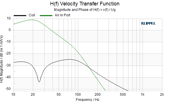
This result window presents all transfer functions related to the velocity. The black curve presents the magnitude of the voice coil velocity over the terminal voltage. The green curve, available for vented systems or systems containing a passive radiator, shows the magnitude of the velocity of air in the vent or the velocity of the passive membrane. All phases are available via curve settings.
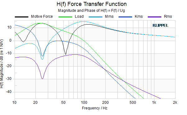
HF(f) Force#
The window Force HF(f) contains all transfer functions related to force. The black curve Fc (motor) presents the motor force divided by the terminal voltage. Additionally, the magnitude of the force-drop over the mechanical mass Mms and over the mechanical stiffness Kms, the mechanical resistance Rms and the mechanical impedance of the acoustical system are depicted. All phases are available via the curve settings.
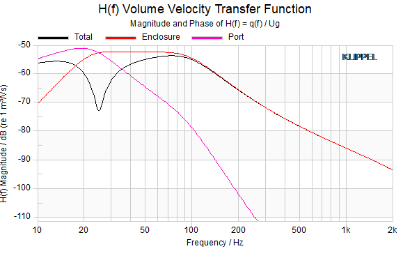
Hq(f) Volume Velocity#
In this window, all curves related to the volume velocity are available. The volume velocity, which is generated by Sd, is depicted as black curve. Additionally, depending on the system, the magnitude of the volume velocity into Cab, into Ral, into the front volume for bandpass systems and into the port is available. The corresponding phases are available via the curve settings.
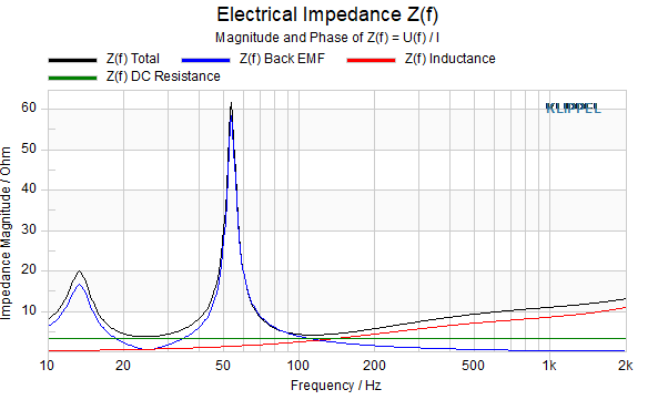
Z(f) Electrical Impedance#
This window shows the magnitudes of the electrical impedance for the total system (black curve), the back EMF (blue curve), the electrical inductance without of Rg and Re (red curve) and the resistances Rg and Re (green curve). All phase information and hidden curves are available via curve settings.
Hg(f) Amplifier#
This window displays the terminal voltage versus the generator voltage. This represents the voltage drop over the output resistance of the amplifier, including the resistance of the cables.
Hequ(f) Equalizer#
This window presents the calculated equalizer transfer function to reach the chosen target transfer behavior. This window is not available if no equalization is activated.
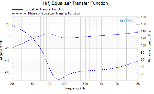
H(f) Group Delay#
This window presents the group delay which is calculated based on the phase information of Hpfar(f,r).
Stimulus related Spectra#
All spectra that are shown by the LSIM module are third-octave spaced.
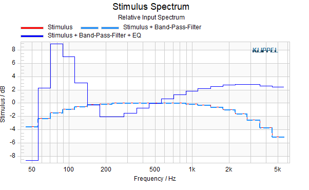
Stimulus Spectrum#
This window contains all relative spectra at the left side of the signal flow chart in front of the amplifier. The spectrum labelled with Stimulus (red) represents the relative input spectrum defined in the property page stimulus. The spectrum Stimulus + Band-Pass-Filter (light blue) shows the band-pass-filtered relative input spectrum. The spectrum Stimulus + Band-Pass-Filter + EQ (blue) illustrates the signal which is applied to the loudspeaker after band-pass and equalization. All these spectra are relative.
LPfar(f) Sound Pressure Level Spectrum#
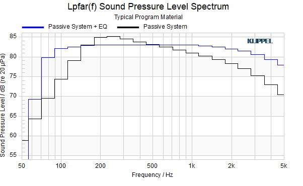
This window corresponds to the window Sound Pressure in Far Field and presents the SPL spectra according to the entered stimulus. The spectrum SPL Loudspeaker (black) represents the SPL of the passive loudspeaker without equalization. The curve SPL Loudspeaker + EQ (blue) is the SPL spectrum including equalization. The spectrum SPL Loudspeaker + EQ + Post-Filter (purple) represents the total system including also the post-filter.
State Spectrum#
The window State Spectrum provides the option to view different state spectra. The state spectrum will be calculated by multiplying the transfer function for the chosen state with the spectrum of the stimulus signal at the terminals. The following states are available:
Voice coil displacement
Voice coil velocity
Voice coil force
Radiated volume velocity
The property page contains a list to specify the desired state.
U(f) Voltage Spectrum#
The window Voltage Spectrum displays the spectrum of the voltage signal at the generator and at the terminals of the loudspeaker. In the case of \(R_g = 0\) both curves are identical.
P(f) Power Spectrum#
This window shows the spectrum of the electrical input power (black) and the acoustical output power (red).
Curve Im/Export#
The required format for curve import and export is the same as other KLIPPEL R&D modules: each curve is represented by two columns of ASCII numbers.
The columns are separated by spaces, and the rows are separated by line breaks. The first column contains the x-values (e.g. frequency), and the second column contains the y-values (e.g. dB). Each row represents a single data point on the curve. The fractional part of the x- and y-values must be separated by a period; a comma is not allowed. If you select any curve with the mouse and press [CTRL + C], it is copied to the clipboard. The two-column text can be copied and/or pasted from any external text editor. Alternatively, use the clipboard editor provided by dB-Lab. It is activated by choosing View Clipboard in the menu. Between the data points, the curve is linearly interpolated. Outside the data point range, the value of the first and the last base point is used respectively.
Supported Modules for Import/Export#