LPM – Linear Parameter Measurement

LPM - Tutorial

Overview

The LPM module determines the linear electrical and mechanical parameters (Thiele-Small parameters) of electro-dynamical transducers. In contrast to the LSI3 – Large Signal Identification (that identifies the large signal parameters) it focuses on the precise measurement of the small signal domain parameters.

See also

E-Learning: Please also refer to the KLIPPEL E-Learning online trainings for more information. Training 1 is dedicated to the LPM measurement.

What is the Goal of This Tutorial?

This tutorial makes you familiar with the LPM module.

The tutorial is divided into three parts.

Viewing LPM Results (Part 1)

In the first part Viewing LPM Results we will show you how to view LPM results already stored in the web example database.

Performing a New LPM (Part 2)

The next part of the tutorial Performing a new LPM provides a step-by-step recipe to measure the electrical and mechanical driver parameters.

Customizing LPM (Part 3)

In the final section Customizing LPM we discuss modifications of the setup parameters to use more powerful features and to improve the performance of the measurement.

In the chapter LPM – Reference you will find more information on the basics of the linear model used as well as a detailed description of the result windows and the configuration of the property pages.

In the last section, you will find information on possible problems, malfunctions and troubleshooting.

Viewing LPM Results (Part 1)

Example data used in this manual is stored in the Web Example database. If not downloaded already, get it from the latest R&D release <https://www.klippel.de/go/current-rnd-release> and open the web-based database.

See also

View Results for general information on how to download this database, open and view results in dB-Lab.

Select the operation:

Transducer Parameter Identification (LSI, LPM, MMT, MSC, BAC, IMP) ‣ Multimedia Woofer (LPM, LSI) ‣ 1 LPM T/S parameter with laser in air

Please refer to the dB-Lab – Software manual section for navigating within or selecting databases.

After double clicking on the operation, the default result windows will be opened.

Table Linear Parameters

The result window shows the electrical and mechanical parameters of the linear driver model, the derived parameters (resonance frequency, loss factors etc.) and the parameter of the suspension creep factor that are determined by the LPM module (if measured with laser method).

The most important results are:

\(R_{\text{e}}\)

Electrical voice coil resistance at DC

\(L_{\text{e}}\)

Frequency independent part of the voice coil inductance

\(f_{\text{s}}\)

Driver resonance frequency

\(M_{\text{ms}}\)

Mechanical mass of driver diaphragm assembly including air load and voice coil

\(Bl\)

Effective force factor (\(Bl\) product)

Z(f) Impedance Magnitude

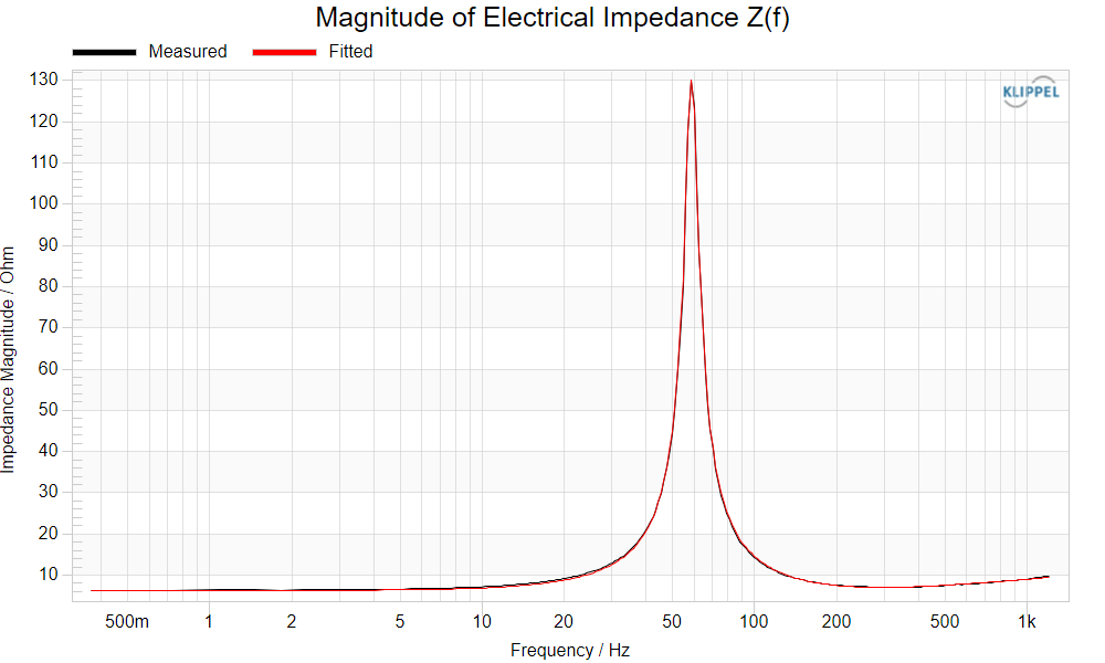
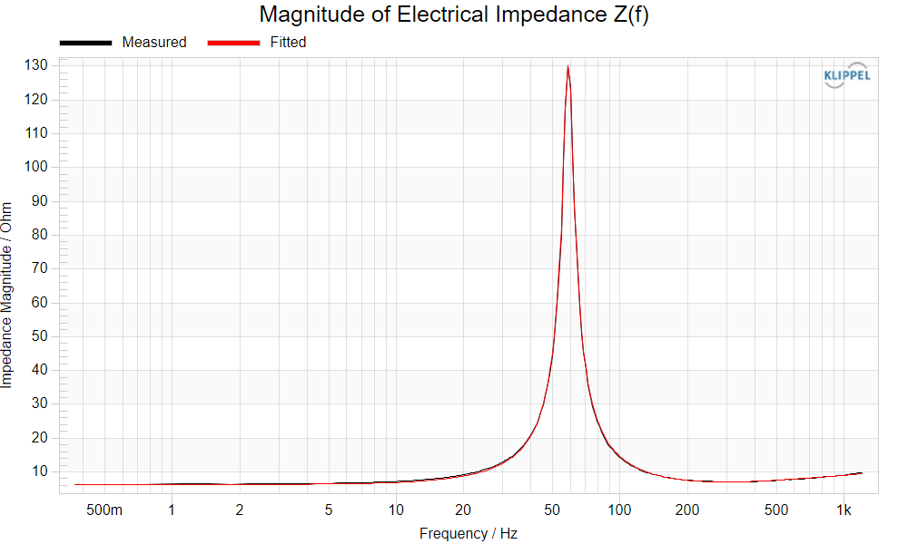
The result window shows the magnitude of the measured and estimated impedance \(Z(f) = \left | \frac{\underline{U}(f)}{\underline{I}(f)} \right |\) where \(U(f)\) is the terminal voltage and \(I(f)\) is the current. The Measured curve is the ratio of the measured spectra \(U(f)\), \(I(f)\) while the Fitted curve is the impedance calculated with the linear driver model using the identified parameters shown above. You can clearly detect the resonance and the increase of impedance at higher frequencies due to the voice coil inductance.

H(f) Displacement Transfer Function

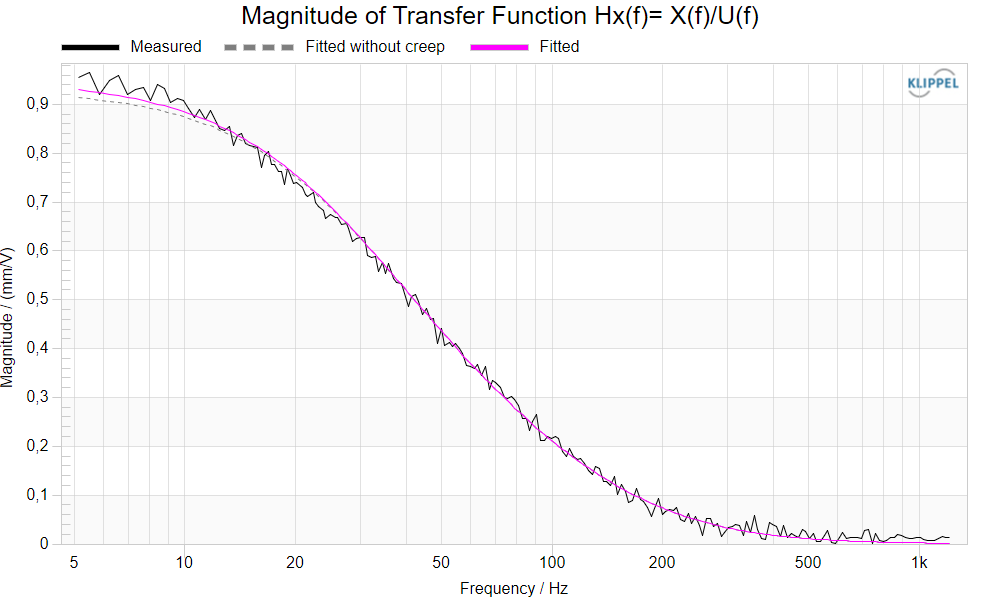
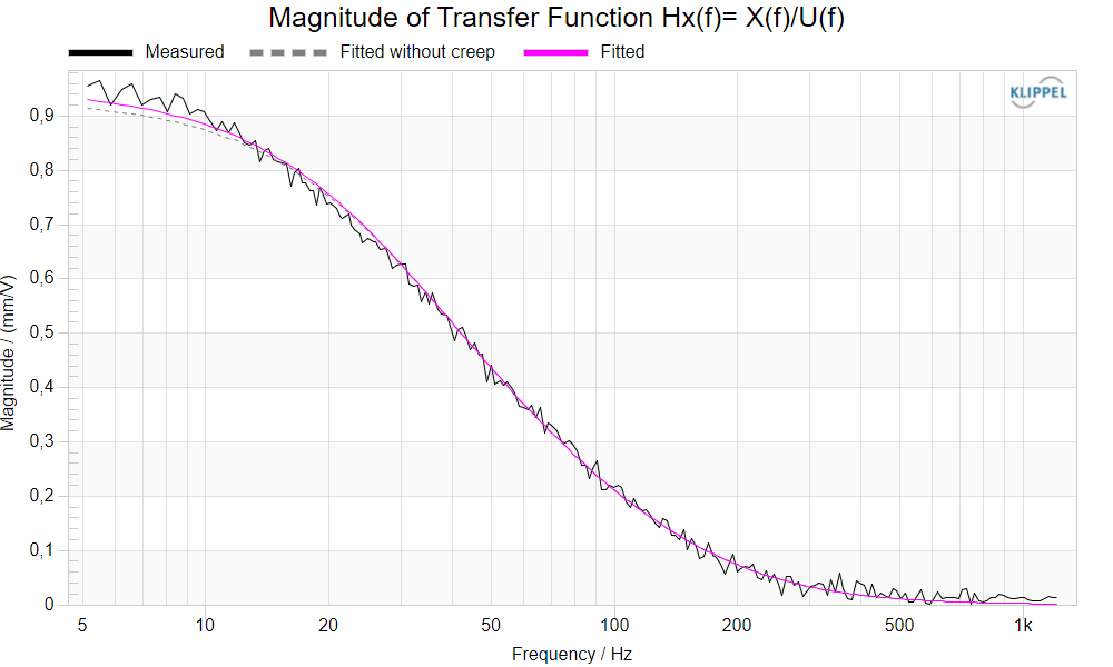
The result window shows the magnitude of the measured and estimated transfer function \(H_{\mathrm{x}}(f) = \left | \frac{\underline{X}(f)}{\underline{U}(f)} \right |\) between the voice coil displacement \(X(f)\) and the terminal voltage \(U(f)\). The Measured curve is the ratio of the acquired spectra \(X(f)\), \(U(f)\) while the Fitted curve is the transfer function based on the linear model using the identified electrical and mechanical parameters as well as the creep parameter.

The creep effect models the low frequency behavior of the suspension system of a loudspeaker. The stiffness is not constant over frequency but decreases for very low frequencies. For more information, see the Linear Modeling of LPM.

The dashed gray curve is based on the conventional model without considering the creep factor.

Spectra of State Variables

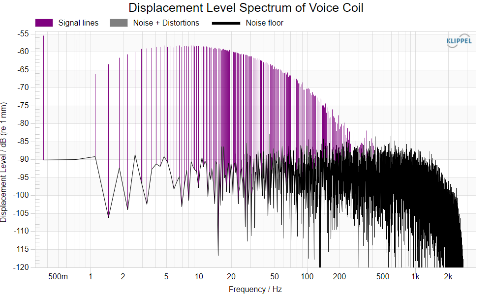
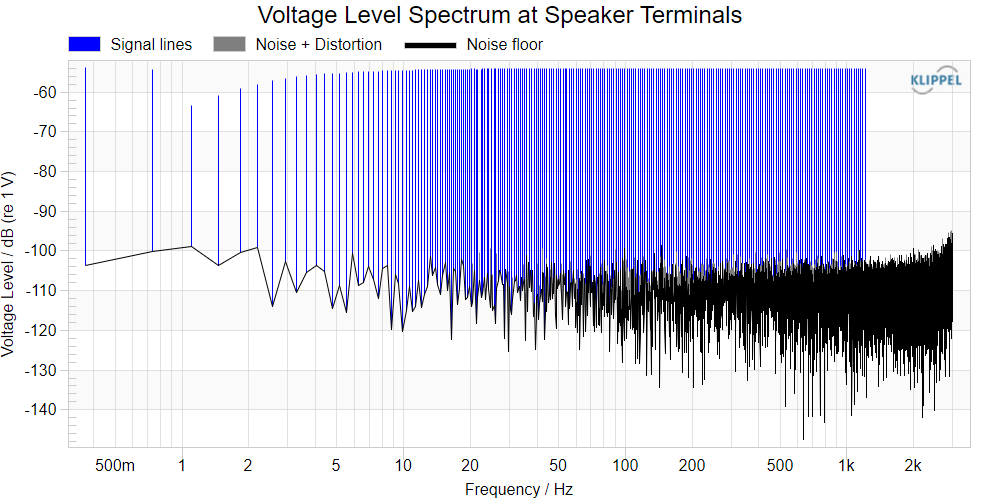
A multi-tone signal used for loudspeaker excitation has some advantages over conventional excitation signals such as MLS. Since we are working with a sparse spectrum, we excite the speaker with logarithmically spaced frequencies and are able to measure the distortion and noise at the unexcited frequencies in the spectrum. The spectra of the measured signals can be viewed in the result windows U(f) Voltage Spectrum, I(f) Current Spectrum, X(f) Displacement Spectrum and p(f) Sound Pressure Spectrum.

Measured Waveforms

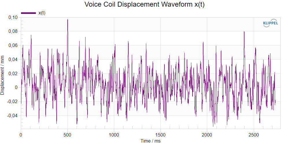
The terminal voltage, input current, voice coil displacement (laser sensor) and sound pressure (microphone) waveforms can be viewed in the result windows u(t) Voltage Waveform, i(t) Current Waveform, x(t) Displacement Waveform and p(t) Sound Pressure Waveform.

Performing a New LPM (Part 2)

In the second part of the tutorial a step-by-step guide is provided to measure the electrical and mechanical driver parameters. We assume that the following standard hardware configuration is available:

• Klippel Analyzer (Power Monitor 8 Hardware does not support LPM Laser method)

• Laser displacement sensor

• Driver mounted in laser stand

• Power Amplifier

If you do not have a laser sensor you may refer to the third part of the tutorial. The section Working without a Laser will give you detailed description.

Setting up the Hardware

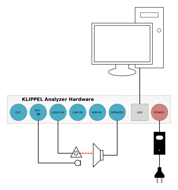
Connect the hardware components as described in the KLIPPEL Analyzer Hardware. Depending on the method you use, you have to connect laser or microphone.

Note

For highly reflective or dark surfaces it may be required to make a dot with white ink (correction fluid) on the diaphragm and adjust the laser to this point. Alternatively, you can use white adhesive tape that can be removed easily after the measurement. See also section Laser Sensors in KLIPPEL Analyzer Hardware manual for more information.

Selecting a Template

Select a meaningful template for your application and selected type of DUT. The provided templates are dedicated for a certain resonance frequency \(f_{\text{s}}\) range. The additional descriptions Subwoofer, Woofer, Midrange, Tweeter are hints not rules. E.g. a headphone transducer could be measured with a woofer template if its resonance frequency \(f_{\text{s}}\) will be in that range.

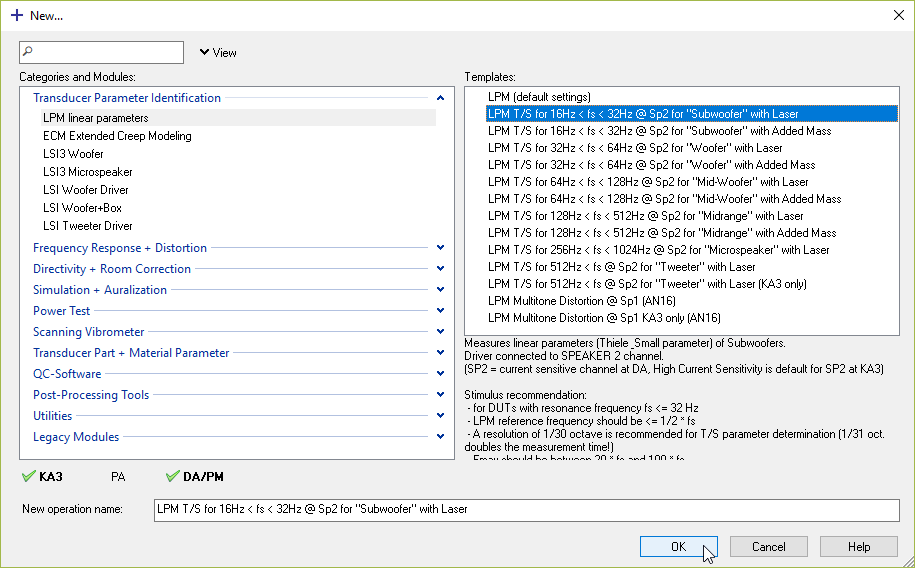
The templates provide reasonable stimulus settings for getting suitable results with a minimal number of measurement iterations and setup adjustments.

Select Setup Parameters

1. Create a new operation and / or object for your own measurements. You should not overwrite the examples in the example database. You find more information in the dB-Lab – Software manual.

2. Select the LPM operation and open the Property Page Driver

   

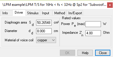
3. Optionally, enter the driver diaphragm area \(S_{\text{d}}\) and the nominal impedance \(Z_{\text{n}}\) to obtain the full set of result parameters. You may find more information about how to measure diaphragm area in How to Measure Diaphragm Area.

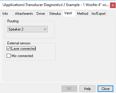
4. Open the Property Page Input and select the connected sensors as well as the used speaker channel. Using the laser, the measurement identifies all of the linear parameters in one step. It is also possible to connect a microphone to measure SPL in the near field, additionally.

   

5. Open Property Page Stimulus shown below

   

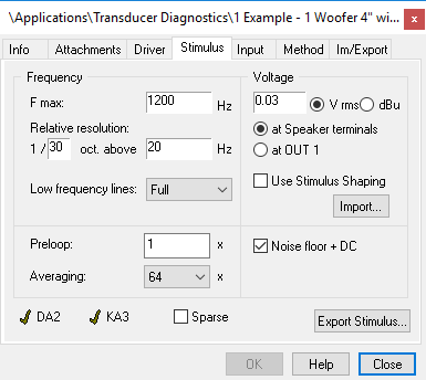
   Specify \(F_{\text{max}}\) (upper frequency range of stimulus), relative resolution, reference frequency and voltage of the excitation signal. The specified voltage is either referred to the speaker terminals (at Speaker terminals) or to the amplifier input (at OUT 1). Select at Speaker terminals. In this case, the amplifier gain is measured prior to the parameter measurement and the excitation signal is adjusted to the measured gain. It is recommended to activate Noise floor monitoring.

Note

Make sure that the selected voltage will not harm the test object. Performing identifications of the linear parameters at higher amplitudes will cause additional parameter variations since the linear model is no longer adequate for the large signal domain.

Select Measurement Method

Open Property Page Method

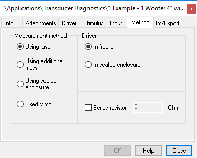
Select Using laser and In free air.

Start Measurement

1. Start measurement by clicking Run

   After testing the amplifier, you will hear the multitone excitation. In the case that the measured signals are too

   low in amplitude or considerably distorted you will get one of the warning messages discussed in part 3

   of this tutorial. To optimize your measurements, you should open the result table Signal Characteristics . In the first line you find

   useful hints to improve the accuracy of the measurement. Also refer to section Reducing Noise Level for further help.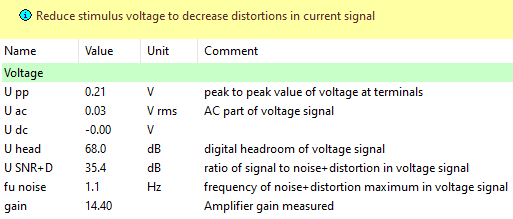

   

2. View all result windows and tables by activating the checkboxes in the result window list. You may also define your own window arrangement and your own setting of default windows (Default windows are opened automatically if double clicked on the operation). For customizing result presentation, refer to the dB-Lab Manual.

3. Repeat the measurement if necessary, by clicking Run

Ensuring Accuracy

To become even more familiar with the LPM it is strongly recommended performing a pair of laser-based and added-mass-based measurements with the same driver at least once. This test does not only provide practical training, it also ensures that the hardware is properly calibrated and connected. By performing both methods of determining the small signal parameters you should obtain a deviation of the \(Bl\) and \(M_{\text{ms}}\) parameters of maximum 5 %. By optimizing the measurement, a typical deviation of 2 % to 3 % is standard and should be aimed. Please find detailed information on performing and optimizing these measurements in the tutorial part 3.

Furthermore, it is recommended to use a reference driver. The calibration and the proper operation of the hardware can be checked easily with a reference driver. We strongly recommend to keep one driver as reference in the shelf and to measure its parameters once in a while. Any deviation of the parameters indicates a hardware or calibration problem.

Customizing LPM (Part 3)

In this part of the tutorial, we discuss modifications of the setup parameters to use more powerful features and improve the performance of the measurement.

Physical Limitations

Influence of Measurement Conditions

The most important results of the linear parameter measurement are the moving mass \(M_{\text{ms}}\) , the force factor \(Bl\) and the DC voice coil resistance \(R_{\text{e}}\). These parameters are almost independent of the amplitude of the excitation signal.

The properties of the suspension depend on many factors (excitation level, time, ambient temperature, humidity). The compliance \(C_{\text{ms}}\) and all derived parameters such as the resonance frequency \(f_{\text{s}}\) and the loss factors \(Q_{\text{ts}}\) and \(Q_{\text{es}}\) vary even in the small signal domain. \(C_{\text{ms}}\) and \(f_{\text{s}}\) may easily vary by 10 % to 20 % with (small signal) excitation level [1] . Furthermore, \(C_{\text{ms}}\) and \(f_{\text{s}}\) can change by 50 % (!) if the temperature is increased from normal ambient temperature to 40°C [2] . However, the parameters \(R_{\text{e}}\) , \(Bl\) and \(M_{\text{ms}}\) should not vary with measurement conditions.

[1]

Klippel, W. and Seidel, U. Fast and accurate measurement of linear transducer parameters. Presented at the 110th Convention of the Audio Engineering Society, Amsterdam, Mai 2001

[2]

Hutt, S. Ambient temperatures influences on OEM automotive loudspeakers. Presented at the 112th Convention of the Audio Engineering Society, Munich, Mai 2002, preprint 5507

Adequate Modeling

The measurement of the linear parameters fails if the model is not adequate for the particular driver. For example, additional electrical components, mechanical sub-resonance and acoustical guides may cause substantial deviations between the measured and expected behavior.

The creep of the suspension can only be measured by a mechanical sensor. This effect may cause substantial errors in the traditional two-step measurements using an additional mass or test enclosure. Both perturbation methods assume that the stiffness is independent on frequency. However, some drivers “forget” 50 % stiffness at frequencies one decade below \(f_{\text{s}}\).

How to Get the Best Performance?

In this section a step-by-step procedure is outlined that maximizes the accuracy of the results. Factors that deteriorate the performance are identified and suggestions are made for improvements.

Precise Calibration

High accuracy of the results requires that the sensors for voltage, current and displacement (if a laser is used) are calibrated carefully. The current and voltage sensors are already factory calibrated.

The calibration of the laser head should be checked more frequently but, in any case, if the head is changed or replaced (see Laser Sensors in the KLIPPEL Analyzer Hardware manual). Any laser calibration error will deteriorate the accuracy of the mechanical parameters. For instance, a 3 % calibration error causes an error of 3 % for \(Bl\) and 6 % for \(M_{\text{ms}}\)!

Amplifier

When using DC-coupled amplifiers make sure to only use the AC coupled output of the analyzer. Avoid amplifiers with a very steep high-pass filter slope (attenuation > 40 dB at 1 Hz relative to pass band). The DC voice coil resistance \(R_{\text{e}}\) is measured at the two lowest frequencies which are selected based on the amplifiers high-pass behavior (< 1 Hz … 4 Hz). Although the attenuation is compensated by up to 27 dB, the signal to noise ratio may be insufficient for this measurement or the lowest test frequencies are too high for an accurate estimation for the DC resistance, in case of a steep amplifier filter slope.

Check Hardware with Reference Driver

The calibration and the proper operation of the hardware can be checked easily with a reference driver. We strongly recommend to keep one driver as reference in the shelf and to measure its parameters once in a while. Any deviation of the parameters indicates a hardware or calibration problem. Please keep the remarks made in section Physical Limitations in mind.

Adjust Laser

Adjust the distance between the laser head and the diaphragm carefully. The adjustment is described in section Laser Sensors in the KLIPPEL Analyzer Hardware manual. Please refer to this chapter for basic considerations on using and installing the laser.

Make sure that the rest position of the diaphragm is in the middle of the laser’s working range. Move the diaphragm slightly with your fingers (if possible) and check that the working range is not exceeded.

To increase reflection, you may apply a white dot (white correction fluid or adhesive tape) on the diaphragm and adjust the laser to this point. The white dot increases the signal to noise ratio of the laser signal considerably, depending on the used laser head. Make sure that the laser is pointed to an approximately perpendicular surface (e.g. center of dust cap or joint). The target may be up to 20° out of perpendicular position without degrading the performance significantly.

Check Mounting of the Driver

Check that the driver is tightly mounted in the laser stand. If the driver is improperly mounted it will vibrate or even change position. Both will falsify the laser measurement. Make sure that no cable, etc. touches the driver or the laser head. It might vibrate slightly during the test and disturb the laser signal.

Use “at Speaker terminals”

Select Voltage: at Speaker terminals in property page Stimulus. In this mode the amplifier low frequency roll-off is measured and compensated (by increasing the excitation level for the attenuated lines). Without roll-off compensation the measurement of the voice coil resistance \(R_{\text{e}}\) may be corrupted due to poor SNR. This will deteriorate the accuracy of the other small signal parameters as well.

Use High-Sensitivity Current Sensing

Depending on the device you are using, there are some special configurations of speaker channel 2 (e.g., higher current sensing sensitivity). Refer to the KLIPPEL Analyzer Hardware manual for your device, to check for more information.

Adjust Frequency Range

Select a meaningful template for your application and selected type of DUT. The provided templates are dedicated for a certain resonance frequency \(f_{\text{s}}\) range. The additional descriptions subwoofer, woofer, midrange, tweeter are hints not rules. E.g. a headphone transducer could be measured with a “woofer” template if its resonance frequency \(f_{\text{s}}\) will be in that range.

Adjust the frequency range in property page Stimulus if this is required by the application or type of DUT.

The maximum frequency \(F_{\text{max}}\) of the excitation signal should be between 20 \(f_{\text{s}}\) and 100 \(f_{\text{s}}\). This will shift the impedance resonance peak to the middle of the logarithmic frequency range which is optimal for curve fitting.

A spectral resolution of 30 lines per octave is required at 0.5 \(f_{\text{s}}\) or lower as the separation of noise and distortion components starts at the selected Reference Frequency. Analyzing the distortion components around resonance frequency \(f_{\text{s}}\) is recommended for ensuring meaningful small signal conditions. Reducing the spectral resolution down to 16 lines per octave could help reducing the distortion as less low frequency content reduces the displacement which activates the distortion. But a lower spectral density also reduces the resonance frequency \(f_{\text{s}}\) fitting accuracy.

Adjust Excitation Level

The excitation voltage needs to be adjusted carefully. Select Noise floor + DC in property page Stimulus. This will invoke an additional noise floor measurement before the main measurement.

The main measurement uses a multi-tone stimulus. Only certain (logarithmically spaced) frequency lines are excited. The output signal of a purely linear system will show only those lines. In case of a nonlinear system (like a driver operated in the large signal domain) additional lines (distortion) are present in the output signal. In the result window I(f) Current Spectrum

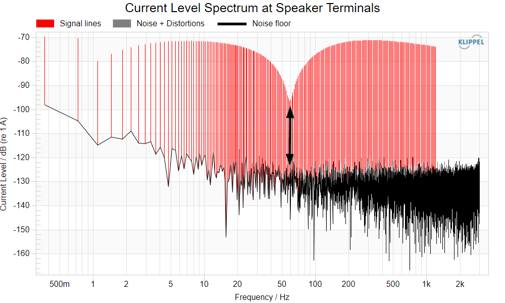
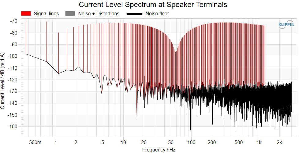
the exited lines are plotted red. As the excitation voltage is almost constant over frequency (voltage driven measurement) the shape formed by the red lines is the inverse of the impedance curve. The additional distortion lines are plotted gray while the noise floor spectrum is depicted as black line. This is very important for adjusting the excitation level. If the level is too high, the distortion lines will exceed the noise floor indicating that the driver is no longer operated in the small signal domain. Very low excitation levels lead to a poor signal to noise ratio.

Therefore, the ratio

\[SNR\: +\: D = \frac{\text{Signal}}{\text{Distortion + Noise}}\]

needs to be maximized for optimal results. Start with a small excitation voltage, e.g. 0.3 V. After the measurement has finished, check the result window I(f) Current Spectrum. The signal lines should exceed the noise floor and the distortion by at least 20 dB. If not, you have probably noticed a warning, saying that the current signal is not properly conditioned. The minimal distance I SNR+D between signal and noise + distortion lines is given numerically in Table Signal Characteristics. Normally it occurs around the resonance frequency (70 Hz in the figure above) due to the resonance notch formed by the signal lines.

Note

The accuracy of the electrical and mechanical parameters is directly related to the SNR+D value. The table below gives the required SNR+D to obtain \(Bl\) with a certain accuracy.

SNR+D	Error
20 dB	10 %
30 dB	3 %
40 dB	1 %

Stimulus Voltage Adjustment

1. If no distortion lines are visible, try to increase the stimulus voltage level until the distortion lines exceed the noise floor slightly.

2. In case of considerable distortion decrease the excitation level until the distortion lines exceed the noise floor slightly. Do not hesitate to apply very small voltages. Values as small as 0.025 V (combined with a high number of averaging) can be an optimal choice for some drivers.

3. If SNR+D is still poor increase the number of averaging. This will reduce the noise floor. Note, that the distortion will not be decreased by more averaging. Adjust the excitation level again till the distortion exceeds the noise floor slightly.

4. If steps 1-3 lead to no improvement check the result window I(f) Current Spectrum for humming components (caused by ground loops). You may also check fi noise (frequency of the minimal SNR+D) in Table Signal Characteristics. In case of ground loops check your setup carefully.

5. The procedure may fail to increase SNR+D above 20 dB if the current spectrum shows a very significant decay (notch) at resonance frequency. This is normally the case if the driver has a high \(Q_{\text{ms}}/Q_{\text{es}}\) ratio. The decay can be flattened considerably if a stimulus shaping is applied, or a resistor of 10-20 Ohm is connected in series to the driver. Proceed as described in section Increasing Signal to Noise Ratio for High Q Drivers in part 3 of the Tutorial. Please follow the outlined procedure exactly to ensure maximal accuracy of the results.

Use the described method 5 only if steps 1-3 definitely fail to produce a proper SNR+D!

Check Laser Spectrum

Open result window X(f) Displacement Spectrum. The displacement spectrum is normally quite constant below resonance frequency \(f_{\text{s}}\) and decreases by 12 dB/octave above \(f_{\text{s}}\). Check the following:

1. Most important is the ratio

   \[SNR\: +\: D = \frac{\text{Signal}}{\text{Distortion + Noise}}\]

   As the displacement signal naturally vanishes in the noise floor at higher frequencies SNR+D is evaluated around and below the resonance frequency only.

   

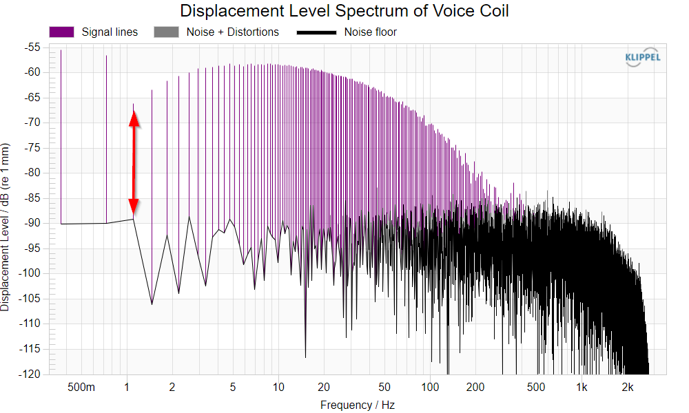
   Displacement spectrum with noise floor and distortion lines

   SNR+D of the displacement should be at least 20 dB. If it is too low try to increase averaging and/or the excitation level. Check the impact of the changes to the current spectrum. Readjust the excitation level if necessary.

   Note

   Note that maximizing SNR+D for the current is more important than maximizing SNR+D for the displacement.

2. The minimal distance X SNR+D between signal and noise + distortion lines is given numerically in Table Signal Characteristics. The calculation ignores signal lines with a level less than 3 dB below the maximum level of the spectrum.

3. Check the distortion present in the displacement spectrum. Normally, there is no distortion in the displacement if there is none in the current. There might be something wrong with the laser if the displacement signal is considerably distorted while the current signal is not.

Check Impedance Fitting

1. Open result window Z(f) Impedance Magnitude. Is the measured curve (black) smooth (not noise corrupted)?

2. Check the overall agreement between measured and fitted curve. Check the agreement at low frequencies (< 5 Hz). This range is most important for fitting the DC voice coil impedance \(R_{\text{e}}\). If the fitting is poor you can specify the \(R_{\text{e}}\) value manually in property page Im/Export. Open Table Linear Parameters and check the fitting error rmse Z. Values between 2 % and 4 % indicate a good fitting.

Check H(f) Fitting

1. Open result window H(f) Displacement Transfer Function. Is the measured curve (black) smooth (not noise corrupted)?

2. Check the agreement between measured and fitted (purple) curve. Open Table Linear Parameters and check the fitting error rmse Hx. Values between 2 % and 4 % indicate a good fitting. Check the measured curve for mechanical resonances which may be caused by the mounting of the driver.

Try to damp the parasitic resonances if they have a significant impact. Make sure that your clamping mechanism is appropriate for the driver’s size. See our Accessories for clamping and driver stand solutions offered by us.

Select Inductance Model

Open property page Im/Export and switch between the different models in the select list Inductance Model. If you are free to choose the inductance model, select the one that gives the lowest fitting errors rmse Z and rmse Hx.

Cross Check with Loaded Mass Method

If you doubt the laser-based linear parameters, perform a second measurement with the loaded mass method (see section Working without a Laser). The results for \(Bl\) and \(M_{\text{ms}}\) should not deviate more than 2-3 % between the two methods.

Speeding up the Measurement

The duration of the measurement depends on a variety of factors. You may accelerate your measurement significantly by considering the following things:

• Use one of the provided templates dedicated to a certain resonance frequency \(f_{\text{s}}\) range of the DUT is recommended for getting valid results without much iterations needed to define a suitable setup. If the resonance frequency \(f_{\text{s}}\) of the DUT allows to choose between two templates, the template dedicated for the higher resonance frequency \(f_{\text{s}}\) range will be operated in a shorter measurement time.

• Decrease the number of averaging in the property page Stimulus. The templates use a medium level of averaging which provides valid results in most cases. But it could be possible that reducing the number of averaging still provides valid results with a sufficient SNR in the sensor signals.

• Starting without averaging and increasing the averaging only in case the SNR needs to be increased is a suitable alternative method.

• Disabling the checkbox Noise floor monitoring in the property page Stimulus reduces the measurement time to the half. This can save time for repeated measurements at known DUT’s. But it is not recommended for the first measurements of new unknown DUT’s, where the separation of noise and distortion is needed to find a valid measurement setup.

• Open the property page Stimulus. Reduce the value of spectral Relative resolution and/or increase the reference frequency.

Note

Changing the upper frequency \(F_{\text{max}}\) of the excitation signal in the property page Stimulus does not influences the duration.

Reducing Noise Level

All the sensors used for measuring sound pressure, displacement, voltage and current add noise to the measured signal. You may reduce any noise component, which is uncorrelated to the stimulus by activating the averaging in the property page Stimulus. We recommend to average over at least 8 measurements.

Importing Mms, Bl, Re

The fitting algorithm fits all parameters automatically to the measured impedance data by default. However, it might be desirable to define fixed values since they are measured or known by other methods. In the property page IMPORT fixed values for \(M_{\text{ms}}\) , \(Bl\) and \(R_{\text{e}}\) can be specified. If the user sets or modifies these values the fitting algorithm tries to fit all other parameters except the fixed ones.

Note

All parameters are refitted if one of the fixed parameters is changed.

How to Set a Fixed Re

If the DC resistance is precisely known, the parameter \(R_{\text{e}}\) can be set to a fixed value in the property page IMPORT. If measuring high-impedance drivers, this method may improve the overall parameter fitting accuracy. The lowest two frequency lines are used for \(R_{\text{e}}\) measurement. Due to the high-pass behavior at the lower band limit of most power amplifiers, the measured results can be noisier than in the pass band. Also, for drivers with a very low resonance frequency (subwoofers), the \(R_{\text{e}}\) measurement at low frequencies may be falsified, especially in combination with a steep amplifier high-pass as found in most Class D amplifiers.

Increasing Signal to Noise Ratio for High Q Drivers

Due to the dip in the current spectrum the signal to noise ratio sometimes decreases rapidly at the resonance frequency. The SNR+D is limited by distortion as usually highest distortion is created around the resonance. This dip can be flattened considerably if a stimulus shaping is applied. This can be realized by using the Stimulus Shaping function, or connecting a resistor of 10 Ohm to 20 Ohm in series to the driver under test. The goal is to decrease the overall displacement, leading to a more linear operation of the driver.

Stimulus Shaping

The distortion created at the resonance frequency is caused by excitation at half, third, etc. of this frequency. Therefore, it is useful, to decrease the excitation signal at those frequencies. A useful shaping is a constant attenuation of -10 dB to -20 dB up to 0.5 \(f_{\text{s}}\), and 0 dB attenuation at \(f_{\text{s}}\). For a driver with a resonance frequency of 100 Hz a suitable shaping would be:

Curve = [
 1    -10
 50   -10
 100  0];

To enter the shaping, open the property page Stimulus, activate Use Stimulus Shaping and enter the shaping by clicking the Edit… Button

Series Resistor

A similar shaping can be applied by adding a series resistor. However, care must be taken as the increased resistance \(R_{\text{e}}\) + \(R_{\text{series}}\) will be measured with less absolute accuracy than \(R_{\text{e}}\) only. This problem can be circumvented if the accurate value of \(R_{\text{e}}\) value is imported for the measurement with the series resistor. The method described below is perfect for measuring \(Bl\) and \(M_{\text{ms}}\) very precisely for drivers that have a high \(Q_{\text{ms}} / Q_{\text{es}}\) ratio (causing a deep current decay at \(f_{\text{s}}\)). In order to use the series resistance, do the following three LPM measurements:

1. First Measurement - LPM Driver: Adjust the setup parameters for an optimal measurement of the driver, and connect the driver

2. Start measurement and wait until the result windows are updated

3. Open Table Linear Parameters and read the value of \(R_{\text{e}}\)

4. Second Measurement - LPM Resistor: Connect the series resistor to the speaker cable (instead of the driver)

5. Start measurement and wait until the result windows are updated

6. Check Impedance Magnitude for a valid fitting in low frequencies. If fitting is good, read the value of Re from Table Linear Parameters. If fitting is not valid, read the impedance of the resistor from the measured impedance.

7. Third Measurement - LPM Resistor + Driver: Open property page Method. Select Series resistor and enter the measured Resistance value \(R_{\text{e}}\) from the Second Measurement (Resistor).

8. Open property page Im/Export and activate an imported \(R_{\text{e}}\) by checking \(R_{\text{e}}\) (Ohm) and enter the \(R_{\text{e}}\) from the first measurement.

9. Connect the speaker cable to the series connection of the resistor and driver.

10. Run the measurement.

11. Now you should get most accurate \(Bl\) and \(M_{\text{ms}}\) results.

Using an Additional Microphone

Select Mic connected in property page Input to measure the sound pressure signal in the near or far field of the driver. While the low frequency response of the driver can be measured by the laser or predicted by the model at high accuracy, the microphone preferably shows the properties at higher frequencies.

The microphone must always be connected to IN1 input channel of the KLIPPEL Analyzer 3 or Distortion Analyzer 2 for LPM measurements.

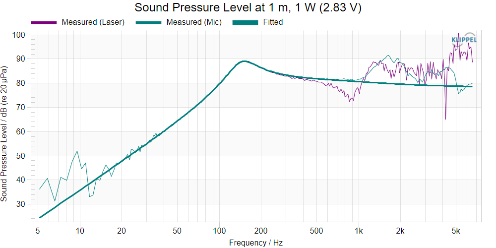
The result window Sensitivity shows the measured (laser and microphone) and predicted driver sensitivity (SPL in 1 m for 1 W electrical input power). The microphone can be placed anywhere in the near field. The microphone sensitivity will be detected automatically.

First, the driver sensitivity is calculated from the displacement signal using the relationship

\[p_{\text{laser}}(t) = \frac{\mathrm{d}x^{2}(t)}{\mathrm{d}t^{2}}\frac{S_{\text{d}}\rho}{2\pi}\]

where \(p_{\text{laser}}(t)\) is the sound pressure signal in 1 m and \(\rho\) is the density of air. After this, the microphone spectrum \(p_{\text{mic}}(f)\) is scaled by a factor \(\alpha\) to match the spectrum \(p_{\text{laser}}(f)\) in the vicinity of 2 \(\cdot f_{\text{s}}\), i.e.

\(p_{\text{laser}}(2f_{\text{s}}) = \alpha p_{\text{mic}}(f_{\text{s}})\).

This leads to a 1 m far field microphone signal. The factor \(\alpha\) accounts for the microphone sensitivity and the near field - far field conversion. Finally, the ratio of \(p_{\text{laser}}(f)\) , \(p_{\text{mic}}(f)\) and the input power spectrum are calculated to get the driver sensitivity.

How to Measure Drivers Mounted in a Sealed Enclosure?

The electrical and mechanical parameters of drivers that are mounted in a sealed enclosure of known volume can be measured with the laser. This is useful if you do not want to remove the driver from the enclosure for the measurement. Due to the stiffness of air enclosed by the box the overall stiffness and the resonance frequency increase. As the force factor \(Bl\) can still be determined correctly with the laser the deviation of the parameters caused by the enclosure can be calculated and compensated if the volume of the enclosure is known. To use this feature, follow these steps:

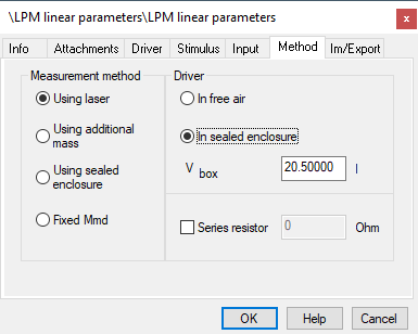
1. Open property page Method and select Using laser in group Measurement method and In sealed enclosure in group Driver. Specify the volume \(V_{\text{box}}\) of the enclosure.

   

2. Start the measurement and wait until the result windows are updated

3. In Table Linear Parameters you will find both the parameters of the system driver + box (influence of the enclosure not removed) as well as the parameters of the sole driver.

How to Use Different Inductance Models

The inductance and the magnetic losses of most drivers are strongly frequency dependent and show a very complex behavior. The LPM supports various common models. They can be selected in property page Im/Export.

See section Inductance Model for detailed information.

Note

Note that the inductance model is used for post-processing only. Switching between models will not invalidate any measurement data. Always use the Shunted inductor model if you want to export the results to the SIM module.

Measuring Distortion

Select Noise floor monitoring in the property page Stimulus to separate the residual noise floor (uncorrelated to the excitation) and nonlinear distortions (harmonics and intermodulation components). It is strongly recommend using always this option, although it doubles the measurement time. With this option you may assess the distortion level produced by the driver and therefore, the validity of linear measurements (where the distortion should be at least 20 dB below the fundamental components).

You may also use the LPM for distortion measurements using multitone excitations. The distortion cannot be separated into harmonic and intermodulation components but the effective distortion pattern may give you clues about the broadband distortion produced by a complex excitation signal. This requires high excitation levels.

Note

The LPM is not recommended anymore for purely acoustical tests. The MTON is a dedicated module for this purpose. Refer to the Application Note AN16 Multi-Tone Distortion for more information.

Adding Comments

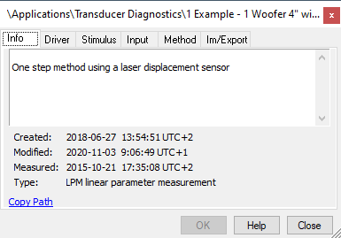
The Info page allows the user to change the name of the measurement and to add a comment to the measurement (comments may be included in the report file). Using templates, the comments are copied to each derived operation. Changing the name may also be done by a slow double click on the operation name in the object tree window.

Working without a Laser

All electrical parameters are obtained from the impedance curve. The module identifies the electrical parameters regardless whether the laser is connected or not. The laser signal is used to identify the mechanical parameters. Although we strongly recommend using the laser, the mechanical parameters may be obtained by performing a second perturbed measurement with an additional mass attached to the driver or the driver mounted in a sealed test enclosure of known volume. Furthermore, it is possible to calculate the mechanical parameters from the impedance curve if the value of \(M_{\text{md}}\) is known (Fixed \(M_{\mathrm{md}}\) method). It is highly recommended to perform a comparison between the classical perturbed method and the laser-based method at least once. The \(Bl\) and \(M_{\text{ms}}\) values should agree with at least 5 % accuracy. This way you make sure that the parameters are identified correctly and the laser is calibrated and used right.

Using an Additional Mass

To obtain the mechanical parameters with the loaded mass method you have to do the measurement in the following steps:

1. Open the property page Method and select the Using additional mass in the group Measurement method and select In free air in the Driver group.

   

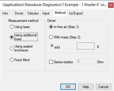
2. Connect the speaker without additional mass.

3. After selecting the other setup parameters in the property pages Stimulus and Input start the first part of the measurement by pressing Run

4. Wait until the result windows are updated.

5. Attach the additional mass to the driver. Be careful to distribute the mass symmetrically over the cone to prevent rocking caused by imbalance and try to fix it tightly to avoid resonances.

6. Open property page Method, select With mass in group Driver and specify the value \(M_{\text{add}}\) of the mass attached to the driver.

   

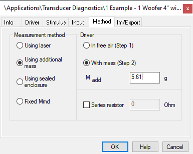
7. Start the second part of the measurement by pressing Run

8. Wait until the result windows are updated. The result windows Z(f) Impedance Magnitude and Impedance Phase will show the results of both measurements. Both the unloaded resonance frequency (\(f_{\text{s}}\)) and the perturbed resonance frequency (\(f_{\text{ct}}\)) are listed in the Table Linear Parameters.

Using a Test Enclosure of Known Volume

Using a test enclosure as perturbation you have perform the following steps:

1. Open the property page Method and select Using sealed enclosure in the group Measurement method and In free air in the Driver group.

2. After selecting the other setup parameters in the property pages Stimulus and Input start the first part of the measurement by pressing Run

3. Wait until the result windows are updated.

4. Open property page Method and select Mounted in sealed enclosure in group Driver and specify the volume V_box of the test enclosure in liter.

5. Start the second part of the measurement by pressing Run

6. Wait until the result windows are updated. The result windows Z(f) Impedance Magnitude and Impedance Phase will show the results of both measurements. Both the free air resonance frequency (\(f_{\text{s}}\)) and the perturbed resonance frequency (\(f_{\text{ct}}\)) are listed in the Table Linear Parameters.

Fixed Mmd

The mechanical parameters can be derived directly from the impedance measurement if the mass \(M_{\text{md}}\) of the voice coil and the diaphragm (without air load) are known.

1. Open the property page Method and select Fixed Mmd in the group Measurement method.

2. Enter \(M_{\text{md}}\) in group Driver.

After selecting the other setup parameters in the property pages Stimulus and Input start the measurement by pressing Run

LPM – Reference

Measurement Technique

The LPM module determines the electrical and mechanical parameters (Thiele-Small parameters) of electro-dynamical transducers. In contrast to the LSI3 – Large Signal Identification (that identifies the large signal parameters) it focuses on the precise measurement of the small signal domain parameters. The electrical parameters are determined by measuring terminal voltage \(u(t)\) and current \(i(t)\) and exploiting the electrical impedance \(Z(f) = \frac{U(f)}{I(f)}\). The mechanical parameters can either be identified using a laser displacement sensor by a second (comparative) measurement where the driver is placed into a test enclosure or by using an additional mass which is attached to it. If \(M_{\text{md}}\) (mass of voice coil and diaphragm without air load) is known the mechanical parameters can be alternatively calculated using the impedance curve and \(M_{\text{md}}\). If the laser is used the displacement of the driver diaphragm is measured in order to exploit the function \(H_{x,u}(f) = \frac{X(f)}{U(f)}\). Therefore, the identification does not require a second measurement and avoids problems due to leakage of the test enclosure or mass attachment. Furthermore, the suspension creep of the driver is identified giving more accuracy of the loudspeaker model at low frequencies.

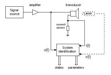
Linear Modeling

The measurement module determines the values of the linear loudspeaker model (Thiele-Small parameters) describing the small signal behavior of electro-dynamic drivers.

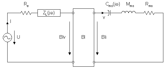
In contrast to the large signal model all parameters of the above equivalent circuit are assumed to be constant (independent of displacement, temperature, etc.).

Inductance Model

The losses due to eddy currents and the magnetic losses of real-world drivers are strongly frequency dependent and show a very complex behavior. The inductance decreases with increasing frequency while magnetic losses produce a resistive loss which increases for rising frequencies. To model the impedance of this lossy inductor three different models are supported. The model used for the impedance curve fitting is selected in property page Im/Export. The inductance model is used for post-processing only. Switching between models will not destroy any measurement data.

LR-2 Model

This lumped parameter model consists of two serially connected inductors \(L_{\text{e}}\) and \(L_{2}\) with \(L_{2}\) shunted by the resistor \(R_{2}\). The impedance of the LR-2 model is given by

\[Z_{\text{L}}(\mathrm{j} \omega) = L_{\text{e}} \cdot \mathrm{j}\omega + \frac{(R_{2} \cdot L_{2} \cdot \mathrm{j}\omega)}{(R_{2} + L_{2} \cdot \mathrm{j}\omega)}\]

with \(\omega = 2 \pi f\). The parameters of the shunted inductor model are \(L_{\text{e}}\) , \(L_{2}\) , \(R_{2}\). The model usually works well for frequencies up to 40 \(f_{\text{s}}\), where \(f_{\text{s}}\) is the resonance frequency of the driver. As it is a lumped parameter model it can be used to simulate the driver in the time domain (see simulation module LSIM – Linear Simulation).

Leach Model

Unlike simple inductors the phase of the impedance of real electro-dynamic transducers is usually significantly smaller than 90 degrees at high frequencies (usually 60-70 degrees). This behavior can be modeled by the lossy inductance model introduced by W. Marshal Leach [3]. The impedance of the Leach inductance model is given by

\[Z_{\text{L}}(\mathrm{j}\omega) = K \cdot (\mathrm{j}\omega)^{n}\]

\[\omega = 2 \pi f\]

Note

Note that the model uses just two parameters (\(K\) and \(n\)).

[3]

Leach, W. M. Loudspeaker voice-coil inductance losses: circuit models, parameter estimation, and effect on frequency respons e J. Audio Eng. Soc., Vol. 50, No. 6, 2002

Wright Model

The relation between real and imaginary part of the Leach model is fixed. Real and imaginary part of the impedance of the Wright model [4]

\[Z_{\text{L}}(\mathrm{j} \omega) = K_{\text{rm}} \cdot \omega^{E_{\text{rm}}} + \mathrm{j} \cdot (K_{\text{xm}} \cdot \omega^{E_{\text{xm}}})\]

\[\quad\omega = 2\pi f\]

can be adjusted separately using the parameters \(K_{\text{rm}}\) , \(E_{\text{rm}}\) and \(K_{\text{xm}}\) , \(E_{\text{xm}}\) respectively. The Wright inductance model usually gives a good fitting over wide frequency ranges. It uses 4 parameters (contrary to the 3 and 2 parameters of the shunted inductor model and the Leach model respectively) and therefore has more degrees of freedom than the other models.

Note

The Leach and the Wright model cannot be used in the simulation module SIM. The SIM module solves the transducer differential equation by numerical integration. The Leach and the Wright model however cannot be represented by a differential equation.

[4]

Wright, J. R. An empirical model for loudspeaker motor impedance. J. Audio Eng. Soc., Vol. 38, No. 10, 1990

Creep of the Suspension

The stiffness \(K_{\text{ms}}(f)\) and compliance \(C_{\text{ms}}(f)\) are assumed to be frequency varying parameters to consider a dynamic property of the mechanical suspension. The mechanical system exposed to a sustained force will show varying displacement versus time (creep effect). Due to the creep effect stiffness of the suspension becomes smaller at lower frequencies. The traditional low-frequency loudspeaker model is expanded to incorporate suspension creep by replacing the simple linear compliance by the dynamic transfer function [5].

\[C_{\text{ms}}(f) = C_{\text{ms}}(f_{s})\Bigl\lbrack 1 - \lambda\log_{10}\Bigl(\frac{f}{f_{s}}\Bigr)\Bigr\rbrack\]

where \(C_{\text{ms}}\) is the linear compliance and \(f_{\text{s}}\) is the driver resonance frequency. There is a straightforward interpretation of the creep factor. The quantity \(\lambda \cdot\) 100 % indicates the increase of the compliance \(C_{\text{ms}}(f_{\text{s}})\) in percentages at low frequencies. For a frequency one decade below the resonance frequency \(f_{\text{s}}\) the compliance \(C_{\text{ms}}(f_{\text{s}})\) is increased by \(\lambda \cdot\) 100 %.

[5]

Knudsen, M. H. and Jensen, J. G. Low-frequency loudspeaker models that include suspension creep. J. Audio Eng. Soc., Vol. 41, No. 1 / 2, 1993

Property Pages

After activating LPM you can open the property pages. These pages present the measurement setup parameters and allow user interaction with the identification process.

Info page

The Info page allows the user to change the name of the measurement and to add a comment to the measurement.

Driver Page

The Driver page contains special transducer parameters that have to be provided by the user.

Stimulus Page

The Stimulus page is used to specify the stimulus (test signal), the number of measurement repetitions (for averaging) and the noise floor monitoring.

Input Page

The connected external devices (Speaker1, Speaker2, laser sensor, microphone) have to be specified

Method Page

The measurement method and the measurement setup are specified in this page

Im/Export Page

The Im/Export page allows the user to import known small signal parameters \(Bl\) , \(M_{\text{ms}}\) , \(R_{\text{e}}\) from other measurements. Furthermore, the whole LPM setup can be exported to or imported from other LPM operations. Finally, the inductance model can be selected.

Info page

The Info page allows the user to add a comment to the measurement (comments may be included in the report file).

Driver Page

The Driver page contains special transducer parameters that have to be provided by the user.

\(S_{\text{d}}\)

The diaphragm area is the effective projected surface area of the driver diaphragm

\(d_{\text{d}}\)

Diaphragm diameter of the driver

Impedance \(Z_{\text{n}}\)

Nominal impedance of the driver

Power \(P_{\text{e}}(\text{max})\)

Maximal nominal input power

Material of voice coil

The kind of material used for the voice coil (copper or aluminum) has to be specified, if known.

Stimulus Page

The Stimulus page gives access to parameters for specifying the stimulus (test signal), the number of measurement repetitions (for averaging) and the noise floor monitoring.

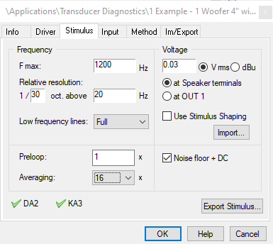
\(F_{\text{max}}\)

Range: \(\leq\) 18000 Hz

Upper bound of frequency range that will be covered by the measurement

Relative resolution

Range: 1 … 99

Number of excited frequencies per octave

Note

Affects stimulus duration together with Relative resolution

Reference frequency

Range: \(\leq\) 18000 Hz

Reference frequency for relative resolution. The specified relative resolution will be ensured for all frequencies above the reference frequency. Below the reference frequency all available spectral lines will be excited.

Note

Affects stimulus duration together with Relative resolution

Low frequency lines

This setting determines whether the frequency band below Reference frequency is excited or not. Full will continue sparse excitation while Re pilot only will add two low frequency tones at very low frequencies for \(R_{\text{e}}\) measurement.

Note

The actual frequency of the low frequency lines (pilot tones) depends on both the stimulus duration (Relative resolution & Reference frequency) as well as the amplifier high-pass decay at low frequencies (\(<\) 1 Hz … 4 Hz).

Voltage

Excitation voltage. The voltage is either the voltage at the speaker terminals or the voltage at the output connector OUT 1. The voltage can be specified in V (RMS) or in dBu.

Shaping

The stimulus spectrum can be further adjusted by importing an inverse shaping curve. The stimulus shaping curve must be given in dB. The shape of the stimulus spectrum is adjusted to the shape of the imported curve. For safety reasons the shaping curve is automatically scaled before applying it to the stimulus. The scaling limits the maximal shaping factor to 0 dB, i.e. the stimulus amplitude will never be increased.

Preloop

Range: \(\geq\) 1

Number of stimulus repetitions before the actual measurement is started. At least one preloop is essential to compensate effects due to time delays.

Averaging

Range: 1 … 128

Number of measurement repetitions for noise reduction.

Voltage: at Speaker terminals

If this option is selected, the specified stimulus voltage is the voltage applied to the speaker terminals. The pass band gain of the amplifier is measured before each measurement at 750 Hz without load and the excitation level is adjusted accordingly. If the measurement is repeated with the same setup parameters, the amplifier gain is not measured again in order to allow fast measurement repetitions. Therefore, the amplifier gain must not be changed during a measurement session.

It is recommended to use Voltage: at Speaker terminals always. In this mode the amplifier low frequency gain decay (high-pass filter slope) is measured and compensated for the two lowest frequency lines (pilot tones) by max. 27 dB. This amplifier’s high-pass behavior also affects the low frequency band limit of the stimulus signal including pilot tones (< 1 Hz … 4 Hz) and thus the accuracy of the voice coil resistance \(R_{\text{e}}\) measurement. Without the gain compensation, the measurement of the \(R_{\text{e}}\) may be corrupted which will affect the accuracy the other small signal parameters as well.

Note

The voltage applied to the speaker terminals will usually be slightly smaller than the specified one. This is because the amplifier gain decreases if a load is connected.

Note

When using the headphone wiring adaptor set provided by KLIPPEL (see Headphone Wiring), both Speaker output terminals will be fed by a single amplifier channel. The second amp channel is not connected in this case. Therefore, you need to physically swap SP1 and SP2 connectors to be able to test both left and right headphone channels, sequentially. Make sure to always set Routing on Input page to Speaker 1.

Voltage: at OUT 1

If this option is selected the specified stimulus voltage is the voltage at the output connector OUT 1.

Note

If an amplifier is used and at OUT 1 is selected the specified stimulus voltage is the voltage at the amplifier input. The level of the amplifier output signal can be considerably higher than the specified level and can possibly destroy your speaker! Please make sure that no amplifier is connected if you use at OUT 1.

Stimulus Shaping

The stimulus can be shaped by importing an attenuation curve (inverse shape), containing the frequency in Hz and the attenuation in dB.

Click the Import… button to import a curve, or Edit… to modify the current shaping curve.

The Use Stimulus Shaping checkbox allows to enable and disable shaping without losing the imported curve.

The curve is entered in two columns, the first column contains the frequency in Hz, the second column the attenuation in dB. The shape will be interpolated, for a step use two very close frequencies (e.g. 100 Hz and 101 Hz).

The shaping curve is relative and does not affect the RMS voltage configured on the Stimulus page (Voltage RMS at OUT 1 / at Speaker terminals).

The effect of the shaping curve can be seen in the U(f) Voltage Spectrum window.

Note

The two lowest frequency lines are excluded from the shaping, and will have the maximum level to allow a reliable measurement of \(R_{\text{e}}\).

You can turn the low frequency lines off completely by setting Low Frequency Lines to Off in the property page Stimulus.

Noise floor + DC Monitoring

If this checkbox is selected an additional noise floor measurement will be performed before the main measurement. This measurement allows furthermore determining offset factors which are important for the correct measurement of the DC components of the measured signals. Therefore, the DC components are shown in Table Signal Characteristics only if the checkbox is selected. The measured noise floor level will be shown as black lines in the result windows U(f) Voltage Spectrum, I(f) Current Spectrum, X(f) Displacement Spectrum and p(f) Sound Pressure Spectrum together with the signal lines acquired during the main measurement.

Export Stimulus

Allows exporting the stimulus signal as wave files (PCM WAV).

The signal will consider all stimulus settings, such as resolution, maximum frequency and frequency shaping. Amplifier compensation and stimulus voltage are not considered, the exported signal is normalized to 95 % of digital full scale.

You can enter a number of repetitions. Which are in addition to the averaging selected on the Stimulus property page. The repetition allows creating a longer continuous signal, as many wave players introduce clicks when playing repeatedly.

Clicking Save will ask for the file name to save under. After you select a folder and enter a file name, the file will be created and shown in Windows Explorer.

Device Measurement Capabilities

On the bottom of the Property Page are two indicators displaying the possibility of measuring with the configured stimulus with either the DA2 or the KA3. If the symbol next to the device is a green tick, the measurement is executable. If the symbol is a red cross the device is not able to execute the measurement. For more information about the reason, click on the device name.

Input Page

On the Input page the relevant signal routing can be modified.

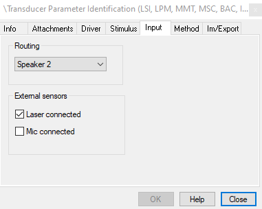
Routing

This setting determines where to which speaker channel of the analyzer the device under test is connected to (Speaker 1 .. Speaker 8). This is relevant for correct measurement of voltage and current.

Note

If you have a hardware version DA 1.2 or higher, speaker channel 2 is equipped with a high-sensitivity current sensor by default. Older versions may be modified on request. It is recommended to use the high-sensitivity current sensor for LPM measurements. With KA3, this setting can be done for each channel of the Speaker Card individually from KA3 Signal Configuration dialog.

Note

When using the headphone wiring adaptor set provided by KLIPPEL (see Headphone Wiring), both Speaker output terminals will be fed by a single amplifier channel. The second amp channel is not connected. Therefore, you need to physically swap SP1 and SP2 connectors to be able to test both left and right headphone channel, sequentially. Make sure to set Routing on the Input page to Speaker 1 always. This does not apply when selecting Voltage: at OUT1 on Stimulus page.

Speaker 3 … Speaker 8 can be used only with a Power Monitor 8 (discontinued). An operation with such a setting cannot be run on a KLIPPEL Analyzer 3 (with one Speaker-Card) or Distortion Analyzer, which provide only two channels.

External Sensors

In case the laser sensor is connected or a microphone is connected to input channel IN1, the corresponding check box can be activated.

The microphone sensitivity can be specified manually or inherit the global sensitivity Managed by dB-Lab (recommended) in group Mic calibration. Remember, that 1 Pascal corresponds to 93.98 dB.

Method Page

On the Method page the method for the identification of mechanical driver parameters is selected.

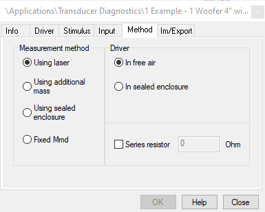
Four different methods are supported:

Measurement method: Using laser

The laser sensor is used to measure the displacement of the driver diaphragm. This single step measurement will determine the suspension creep parameter as well. It avoids a second measurement and thus avoids problems due to leakage of the test enclosure and mass attachment. The driver parameters can be identified for drivers in free air (see part 2 of the Tutorial) as well as for drivers mounted in a sealed enclosure (see section How to Measure Drivers Mounted in a Sealed Enclosure? in part 3 of the Tutorial).

Measurement method: Using additional mass

The mechanical parameters are identified in a two-step procedure. First a reference measurement is performed in free air. The mechanical parameters are determined by comparing it with a second measurement where an additional mass is attached to the driver’s diaphragm (see section Working without a Laser in part 3 of the Tutorial).

Measurement method: Using sealed enclosure

The mechanical parameters are identified in a two-step procedure. First a reference measurement of the driver in free air is performed. The mechanical parameters are determined by comparing it with a second measurement where the driver is mounted in a sealed test enclosure (see section Working without a Laser in part 3 of the Tutorial).

Measurement method: Fixed Mmd

This single step mode can be used if the mass \(M_{\text{md}}\) of the voice coil and diaphragm (excluding air load) is known. The mechanical parameters are calculated from the measured impedance curve and \(M_{\text{md}}\) (see section Working without a Laser in part 3 of the Tutorial).

Driver

The driver can be measured either in free air, with an additional test mass attached or mounted in a sealed test enclosure (see above). Please select In free air, With mass or In sealed enclosure accordingly. In the second and the third case the mass \(M_{\text{add}}\) attached and the volume \(V_{\text{box}}\) of the test enclosure have to be quantified.

Series resistor

Due to the dip in the current spectrum the signal to noise ratio sometimes decreases rapidly at the resonance frequency. The dip can be flattened considerably if a resistor of 10 Ohm to 20 Ohm is connected in series to the driver under test. Furthermore, the series resistor will decrease the overall displacement leading to a more linear operation of the driver. This method is perfect for measuring \(Bl\) and \(M_{\text{ms}}\) very precisely for drivers that have a high \((\frac{Bl}{R_{\text{mx}}})^{2}\) and a low \(R_{\text{e}}\) (causing a strong decay at \(f_{\text{s}}\)). See section How to Get the Best Performance? . Use a series resistor to increase signal to noise ratio in part 3 of the tutorial for further information.

Im/Export Page

All LPM setup parameters can be imported from and exported to other LPM operations:

Export whole LPM setup to the clipboard

Import whole LPM setup from the clipboard

Furthermore, the measured electrical and mechanical driver parameters can be exported to other modules like LSI3 – Large Signal Identification and various simulation modules such as LSIM – Linear Simulation or SIM – Simulation. To do so, press the Export button after LPM has finished. This will copy the driver parameters (together with the LPM setup parameters) to the clipboard. Open the target operation and press the Import button in property page Im/Export. All driver parameters of interest are now read from the clipboard (the LPM setup parameters are ignored as they can only be read by LPM operations). All compatibly modules for import/export a listed in section Supported Modules for Im/Export.

Additionally, you can configure further post-processing options here.

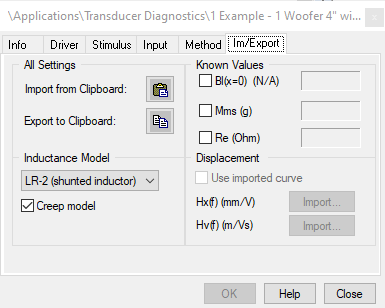
Known Values

If known, some small signal parameters such as force factor \(Bl\) can be user defined to override the measured values. This will cause LPM to recalculate the small signal parameters using the user defined value. For instance, if you have a precisely measured \(R_{\text{e}}\) and want LPM to use this value.

The \(R_{\text{e}}\) value override causes LPM to recalculate the complete linear parameter set. \(Bl\) or \(M_{\text{ms}}\) override will cause LPM to recalculate only the mechanical parameters, while the electrical parameters are kept constant. Overriding both \(Bl\) and \(M_{\text{ms}}\) simultaneously overdetermines the calculation, so it is recommended to only use \(Bl\) or \(M_{\text{ms}}\) override, not both. The choice between \(Bl\) or \(M_{\text{ms}}\) override depends on which value was directly determined and which value was calculated from the other.

(Laser measurement = use \(Bl\) override / Added mass measurement = use \(M_{\text{ms}}\) override)

Bl

\(Bl\) in N/A

Range: 0 \(< Bl <\) 100 N/A

Force factor at the rest position of the voice coil

Re

\(R_{\text{e}}\) in Ohm

Range: 0 \(< R_{\text{e}} <\) 100 Ohm

Electrical DC-resistance of the cold voice coil

Mms

\(M_{\text{ms}}\) in Gram

Range: 0 \(< M_{\text{ms}} <\) 1000 g

Moving mass of driver diaphragm assembly including voice-coil and air load (overwrites \(M_{\text{md}}\) in the Fixed Mmd measurement method)

Inductance Model

This list is dedicated to selecting the inductance model used for the impedance fitting. Three different models are supported. See section Inductance Model for further information.

1. LR-2 model: This model usually gives a good fitting of the impedance in the frequency range up to 40 \(f_{\text{s}}\). You have to select this model if you want to perform a simulation with the SIM module based on the measured LPM results.

2. Leach model: The model gives good impedance fitting especially at high frequencies while using only two model parameters. The model is not supported by the SIM module as it cannot be represented by a differential equation.

3. Wright model: This model normally gives a good fitting over wide frequency ranges, but it is also more susceptible to fitting problems than the less complex models. The model is not supported by the SIM module as it cannot be represented by a differential equation.

Creep model

If this checkbox is selected the suspension creep factor \(\lambda\) will be included into the driver model.

Displacement Hx(f), Hv(f) Import

In addition to the laser used during the measurement, you can import the transfer function \(H_{\mathrm{x,u}}(f)\) or \(H_{\mathrm{v,u}}(f)\) from an external measurement.

To import a curve, click the respective Import… or Edit… button. The checkbox Use imported curve allows switching between measured and imported curve.

If enabled, the imported curve will be used for calculation of the mechanical model, as displayed in the Table Linear Parameters. The curve \(H_{\mathrm{x}}(f)\) will also be shown in the H(f) Displacement Transfer Function result window.

Result Windows

Table Linear Parameters

The result window shows the electrical and mechanical parameters of the linear driver model, the derived parameters (resonance frequency, loss factors etc.) and the parameter of the suspension creep factor that are determined by the LPM module. See section Algorithms and Equations for detailed information about the algorithms used for calculating the electrical and mechanical parameters.

Electrical Parameters

Re

\(R_{\text{e}}\) in Ohm

electrical voice coil resistance at DC

Le

\(L_{\text{e}}\) in mH

frequency independent part of voice coil inductance

L2

\(L_{2}\) in mH

para-inductance of voice coil

R2

\(R_{2}\) in Ohm

electrical resistance due to eddy current losses

Cmes

\(C_{\text{ms}}\) in µF

electrical capacitance representing moving mass

Lces

\(L_{\text{ces}}\) in mH

electrical inductance representing driver compliance

Res

\(R_{\text{es}}\) in Ohm

resistance due to mechanical losses

fs

\(f_{\text{s}}\) in Hz

driver resonance frequency

fm

\(f_{\text{m}}\) in Hz

resonance frequency of the driver with additional mass attached

fct

\(f_{\text{ct}}\) in Hz

resonance frequency of the driver operated in sealed enclosure

Mechanical Parameters

Mms

\(M_{\text{ms}}\) in g

mechanical mass of driver diaphragm assembly including air load and voice coil

Mmd (Sd)

\(M_{\text{ms}}(S_{\text{d}})\) in g

mechanical mass of voice coil and diaphragm without air load

Rms

\(R_{\text{ms}}\) in kg/s

mechanical resistance of total-driver losses

Cms

\(C_{\text{ms}}\) in mm/N

mechanical compliance of driver suspension

Kms

\(K_{\text{ms}}\) in N/mm

mechanical stiffness of driver suspension

Bl

\(Bl\) in N/A

force factor (\(Bl\)-product)

Lambda S

\(\lambda_{\text{s}}\)

suspension creep factor

Loss factors

Qtp

\(Q_{\text{tp}}\)

total \(Q\)-factor considering all losses

Qms

\(Q_{\text{ms}}\)

mechanical \(Q\)-factor of driver in free air considering \(R_{\text{ms}}\) only

Qes

\(Q_{\text{es}}\)

electrical \(Q\)-factor of driver in free air considering \(R_{\text{e}}\) only

Qts

\(Q_{\text{ts}}\)

total \(Q\)-factor considering \(R_{\text{e}}\) and \(R_{\text{ms}}\) only

Other Parameters

Vas

\(V_{\text{as}}\) in Liter

equivalent air volume of suspension

n0

\(n_{0}\) in %

reference efficiency of electro-acoustical conversion (\(2 \pi\) - radiation load)

Lm

\(L_{\text{m}}\) in dB

characteristic sound pressure level (SPL at 1 m for 1 W @ \(R_{\text{e}}\))

Lnom

\(L_{\text{nom}}\) in dB

nominal sensitivity (SPL at 1 m for 1 W @ \(Z_{\text{n}}\))

rmse Z

\(\mathrm{RMSE}_{Z}\) in %

fitting error (RMS) of the driver impedance \(Z(f)\)

rmse Hx

\(\mathrm{RMSE}_{Hx}\) in %

fitting error RMS of the transfer function \(H_{x,u}(f)\)

Series resistor

\(Z\) in Ohm

resistance of series resistor

Sd

\(S_{\text{d}}\) in cm²

diaphragm area

Madd

\(M_{\text{add}}\) in g

additional mass attached to the driver

Vbox

\(V_{\text{box}}\) in Liter

volume of test enclosure

Note

The mass \(M_{\text{md}}\) is calculated by subtracting the mass \(M_{\text{ml}}\) of the moving air from \(M_{\text{ms}}\). The air load \(M_{\text{ml}}\) cannot be measured directly. However, it can be calculated for a piston like diaphragm moved in free air if the diaphragm area \(S_{\text{d}}\) is known. The notation Mmd (Sd) is used to emphasize this dependency.

The mechanical stiffness is the reciprocal of the compliance

\[K_{\text{ms}} = \frac{1}{C_{\text{ms}}}\]

The loss factors are defined as follows:

\[Q_{\text{ms}} = 2 \pi f_{\text{s}} C_{\text{mes}} R_{\text{es}}\]

\[Q_{\text{es}} = 2 \pi f_{\text{s}} C_{\text{mes}} R_{\text{e}}\]

\[Q_{\text{eps}} = 2 \pi f_{\text{s}} C_{\text{mes}} \lbrack R_{\text{e}} + \mathfrak{R}\{Z_{\text{fitted}}(f_{\text{s}})\} \rbrack\]

\[Q_{\text{ts}} = \frac{Q_{\text{ms}}Q_{\text{es}}}{Q_{\text{ms}} + Q_{\text{es}}}\]

\[Q_{\text{tp}} = \frac{Q_{\text{ms}}Q_{\text{eps}}}{Q_{\text{ms}} + Q_{\text{eps}}}\]

The derived parameters are given by

\[V_{\text{as}} = \rho c^{2} S_{\text{d}}^{2} C_{\text{ms}}\]

\[n_{0} = \frac{\rho (Bl)^{2} S_{\text{d}}^{2}}{2 \pi c R_{\text{e}} M_{\text{ms}}^{2}}\]

\[L_{\text{m}} = 112.2 + 10 \log_{10}(n_{0})\]

\[L_{\text{nom}} = L_{\text{m}} + 10 \log_{10}\Bigl(\frac{Z_{\text{n}}}{R_{\text{e}}}\Bigr)\]

where \(\rho = 1.189 \, \frac{\text{kg}}{\text{m}^3}\) is the density of air, \(S_{\text{d}}\) denotes the effective diaphragm area and \(c = 345 \, \frac{\text{m}}{\text{s}}\) the speed of sound.

The fitting measures quantify the disagreement between measured and fitted curves

\[\mathrm{RMSE}_{Z} = \sqrt{\frac{\sum\limits_{i = 0}^{N - 1} w(f_{i}) \vert Z_{\text{fit}}(f_{i}) - Z_{\text{meas}}(f_{i}) \vert^{2}}{\sum\limits_{i = 0}^{N - 1} w(f_{i}) \vert Z_{\text{meas}}(f_{i}) \vert^{2}}}\]

\[\mathrm{RMSE}_{Hx} = \sqrt{\frac{\sum\limits_{i = 0}^{N - 1} w(f_{i}) \vert H_{x,\text{fit}}(f_{i}) - H_{x,\text{meas}}(f_{i}) \vert^{2}}{\sum\limits_{i = 0}^{N - 1} w(f_{i}) \vert H_{\text{x,meas}}(f_{i}) \vert^{2}}}\]

The weighting

\[w(f) = \frac{\frac{f}{f_{\text{s}}}}{(\frac{f}{f_{\text{s}}} + 1)^{2}}\]

emphasizes fitting errors near the resonance frequency. Fitting errors between 2 % and 4 % indicate a good fitting.

Table Signal Characteristics

This table summarizes important statistical characteristics (peak value, headroom, SNR+D, …) of the state variables (voltage, current, displacement and sound pressure). This information is helpful for assessing the working point of the driver (small signal domain versus large signal domain) and to detect any malfunction operation (microphone or laser not connected, humming from ground loop).

Voltage

U pp

\(U_{\text{pp}}\) in V

peak to peak value of voltage at terminals

U ac

\(U_{\text{ac}}\) in V

AC part of voltage signal (RMS)

U dc

\(U_{\text{dc}}\) in V

DC part of voltage signal (only shown if Noise floor + dc monitoring is selected in property page Stimulus)

U head

\(U_{\text{head}}\) in dB

digital headroom of voltage signal

U SNR+D

\(U_{\text{SNR + D}}\) in dB

ratio signal / (noise + distortion) in voltage signal

fu noise

\(f_{\text{u,noise}}\) in Hz

frequency of noise maximum in voltage signal

Gain

Amplifier gain measured

Current

I pp

\(I_{\text{pp}}\) in A

peak to peak value of current at terminals

I ac

\(I_{\text{ac}}\) in A

AC part of current signal (RMS)

I dc

\(I_{\text{dc}}\) in A

DC part of current signal (only shown if Noise floor + dc monitoring is selected in property page Stimulus)

I head

\(I_{\text{head}}\) in dB

digital headroom of current signal

I SNR+D

\(I_{\text{SNR + D}}\) in dB

ratio of signal to noise + distortion in current signal

fi noise

\(f_{\text{i,noise}}\) in Hz

frequency of noise maximum in current signal

Displacement

X pp

\(x_{\text{pp}}\) in mm

peak to peak value of displacement signal

X ac

\(x_{\text{ac}}\) in mm

AC part of current signal (RMS)

X dc

\(x_{\text{dc}}\) in mm

DC part of displacement signal (only shown if Noise floor + dc monitoring is selected in property page Stimulus)

X head

\(X_{\text{head}}\) in dB

digital headroom of displacement signal

X SNR+D

\(x_{\text{SNR + D}}\) in dB

ratio of signal to noise+distortion in displacement signal

fx cutoff

\(f_{\text{x,cutoff}}\) in Hz

frequency of highest valid line in displacement signal

SPL

p pp

\(p_{\text{pp}}\) in mV

peak to peak value of microphone signal

p ac

\(p_{\text{ac}}\) in mV

AC part of microphone signal (RMS)

p head

\(p_{\text{head}}\) in dB

digital headroom of microphone signal

p sum level

\(L_{p,\text{sum}}\) in dB

sum level of microphone signal

p mean level

\(L_{p,\text{mean}}\) in dB

mean level of microphone signal

Measurement

f sample

\(f_{\text{sample}}\) in Hz

sample frequency

N stim

\(N_{\text{stim}}\) in number of samples

stimulus length

Z(f) Impedance Magnitude, Z(f) Impedance Phase

The two result windows show the magnitude and the phase response of the measured and estimated impedance \(Z(f) = \frac{U(f)}{I(f)}`where :math:`U(f)\) is the terminal voltage and \(I(f)\) is the current. The black curve is the ratio of the measured spectra \(U(f)\) , \(I(f)\) while the red curve is the impedance of the linear driver equivalent circuit using the linear model and the identified electrical parameters.

H(f) Displacement Transfer Function

The result window shows the magnitude of the measured and estimated transfer function \(H_{\mathrm{x,u}}(f) = \frac{X(f)}{U(f)}\) between the voice coil displacement \(X(f)\) and the terminal voltage \(U(f)\). The black curve is the ratio of the measured spectra \(X(f)\), \(U(f)\) while the magenta curve is the transfer function based on the linear driver equivalent circuit using the identified electrical and mechanical parameters as well as the creep parameter. The dashed gray curve is based on the conventional model without considering the creep factor.

If you have imported an externally measured \(H_{\mathrm{x,u}}(f)\) or \(H_{\mathrm{v,u}}(f)\) curve on property page Im/Export and you have activated to use the imported curve for calculations, the \(H_{\mathrm{x,u}}(f)\) curve from the import is displayed instead.

Note

From dB-Lab version 206 the frequency range for the creep fitting algorithm was limited to low frequencies where creep is active. For some measurements the \(H_{\mathrm{x,u}}(f)\) fitting at higher frequencies may appear worse compared to results displayed in previous versions of dB-Lab. However, this change leads to more accurate creep factors, and the seemingly better fit in previous versions is not physically correct. You may need to improve measurement conditions for a better general fitting. See Application Note 25: Maximizing LPM Accuracy for more information.

Sensitivity

The result window shows the sound pressure level in 1 meter distance obtained for a nominal input power of 1 Watt. The thin green curve is directly measured by a microphone in the near field of the driver. The solid green curve is calculated by the identified linear speaker model. The purple curve is derived from the laser measurement by differentiating the displacement \(x(t)\) twice and considering the diaphragm area \(S_{\text{d}}\) to calculate the moved volume velocity. All curves are calculated using the nominal impedance \(Z_{\text{n}}\) of the driver.

Z(f) Lossy Inductance

The window shows magnitude and phase of the impedance \(Z_{\text{P}}(f)\) due to the voice coil inductance and eddy current losses. The curves are obtained by removing \(R_{\text{e}}\) and the impedance \(Z_{\text{R}}\) that corresponds to the back induced voltage (caused by the voice coil movement) from the measured impedance \(Z(f)\). \(Z_{\text{R}}\) is calculated using the identified parameters \(C_{\text{mes}}\) , \(L_{\text{ces}}\) and \(R_{\text{es}}\).

\[Z_{\text{P}}(\textrm{j} \omega) = Z_{\text{meas}}(\textrm{j} \omega) - R_{\text{e}} - (\frac{1}{\textrm{j} \omega C_{\text{mes}}} + \textrm{j} \omega L_{\text{ces}} + R_{\text{es}})\]

u(t), i(t), x(t), p(t)

The measured terminal voltage, input current, voice coil displacement (laser sensor) and sound pressure (microphone) waveform signals are displayed versus time.

Spectra of the Measured Signals

A multi-tone signal used for loudspeaker excitation has some advantages over conventional excitation signals such as MLS. Since a sparse spectrum is used, the speaker is excited with a logarithmic distance between the tones and by this, the distortion and noise can be monitored at the unexcited frequencies in the spectrum.

U(f) Voltage Spectrum

The result window shows the multi-tone spectrum of the voltage at the terminals. The blue lines represent the fundamental components excited by the stimulus. The black Noise floor lines represent the residual measurement noise caused by the voltage sensor. If the gray Noise + Distortion exceeds the residual noise floor we see the distortions generated by the nonlinearities of the power amplifier. The fundamental components should be constant in amplitude. At lower frequencies you see the roll off of the AC-coupled amplifier.

I(f) Current Spectrum

The result window shows the multi-tone spectrum of the current at the terminals. The red lines represent the fundamental components excited by the stimulus. Note the notch of the spectrum at the resonance frequency of the driver. The black Noise floor lines indicate the residual noise caused by the measurement system (current sensor). Increasing the number of averaging will further reduce the residual noise line. If the gray Noise + Distortions lines exceed the residual noise floor we see the distortions generated by the nonlinearities of the speaker (assuming that the power amplifier is sufficiently linear). These components are independent of the number of averaging.

X(f) Displacement Spectrum

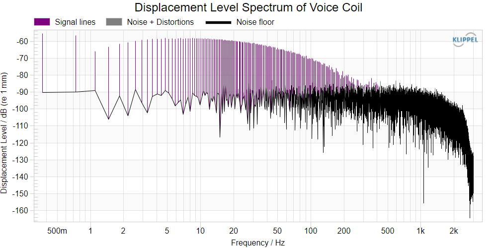
The result window shows the multi-tone spectrum of the voice coil displacement measured with the laser sensor. The magenta lines represent the fundamental components excited by the stimulus. Note the 12 dB/octave decay of the displacement spectra above the resonance frequency of the laser. The black Noise floor lines indicate the measurement noise. Increasing the number of averaging will further reduce the residual noise line. If the gray Noise + Distortion exceeds the residual noise floor we see the distortions generated by the nonlinearities of the speaker. These components are independent of the number of averaging.

p(f) Sound Pressure Spectrum

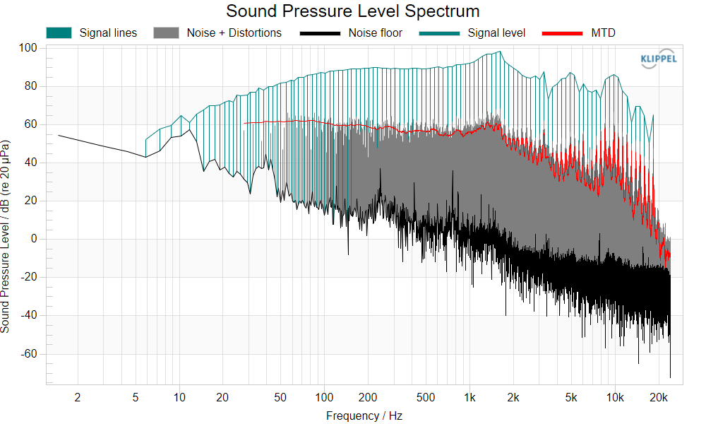
The result window shows the multi-tone spectrum of the sound pressure measured with the microphone. They green lines represent the fundamental components excited by the stimulus. The black Noise floor lines indicate the ambient noise during the measurement. The gray Noise + Distortions are the nonlinear distortion components generated by the speaker. The red multi-tone distortion (MTD) depicts the moving average of the nonlinear distortion components according to IEC 60268-21.

Multitone Distortion

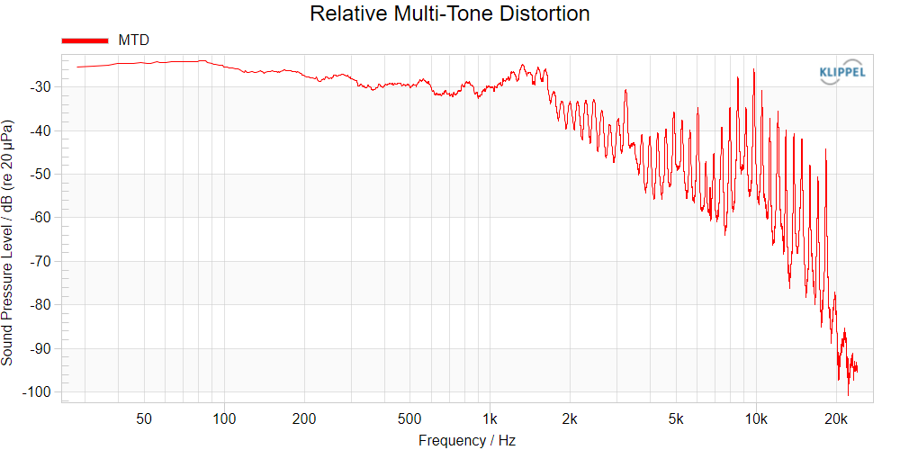
The result window shows the ratio of the nonlinear multi-tone distortion (MTD) to the mean level of the microphone signal. This curve can be seen as a fingerprint of the nonlinear loudspeaker characteristics.

Algorithms and Equations

Laser-based Method

1. Fit \(R_{\text{e}}\) , \(C_{\text{mes}}\) , \(L_{\text{ces}}\) , \(R_{\text{es}}\) , \(L_{\text{e}}\) , \(L_{2}\) , \(R_{2}\) , [\(n\) , \(K\)] , [\(K_{rm}\) , \(E_{rm}\) , \(K_{xm}\) , \(E_{xm}\)] to magnitude and phase of the measured impedance curve \(Z(f) = \frac{U(f)}{I(f)}\)

   Fix \(R_{\text{e}}\) to \(R_{\text{e}\: \text{import}}\) during fitting if import is activated.

2. Calculate \(f_{\text{s}}\) and loss factors

3. Fit \(Bl\) and \(\lambda\) to the magnitude of the measured curve \(H_{\mathrm{x}}(f) = \frac{X(f)}{U(f)}\)

4. Replace \(Bl\) by \(Bl_{\text{import}}\) if import is activated

5. \[M_{\text{ms}} = \frac{Q_{\text{es}}Bl^{2}}{2 \pi f_{\text{s}} R_{\text{e}}}\]

6. Replace \(M_{\text{ms}}\) by \(M_{\text{ms}\: \text{import}}\) if mass import is activated. If mass import is activated, but \(Bl\) import is disabled, then calculate \(Bl = \sqrt{\frac{M_{\text{ms}\: \text{import}} 2 \pi f_{\text{s}} R_{\text{e}}}{Q_{\text{es}}}}\)

7. \[C_{\text{ms}} = \frac{1}{(2 \pi f_{\text{s}})^{2} M_{\text{ms}}}\]
8. \[K_{\text{ms}} = \frac{1}{C_{\text{ms}}}\]
9. \[R_{\text{ms}} = \frac{2 \pi f_{\text{s}} M_{\text{ms}}}{Q_{\text{ms}}}\]
10. \[M_{\text{md}}(S_{\text{d}}) = M_{\text{ms}} - 1.13 \cdot S_{\text{d}}^{\frac{3}{2}}\]

11. Calculate \(V_{\text{as}}\) , \(\eta_{0}\) , \(L_{\text{m}}\)

Laser-based Method with Driver Mounted in Sealed Enclosure

1. Determine the electrical and mechanical parameters of the system driver + box (\(R_{\text{e}}\) , \(C_{\text{mect}}\) , \(L_{\text{cect}}\) , \(R_{\text{ect}}\) , \(L_{\text{e}}\) , \(L_{2}\) , \(R_{2}\) , [\(n\) , \(K\)] , [\(K_{rm}\) , \(E_{rm}\) , \(K_{xm}\) , \(E_{xm}\)] \(Bl\) , \(\lambda_{\text{ct}}\) , \(M_{\text{mct}}\) , \(C_{\text{mct}}\) , \(K_{\text{mct}}\) , \(R_{\text{mct}}\) ) as described above in section Laser-based Method.

2. \[K_{\text{ms}} = K_{\text{mct}} - \frac{\rho c^{2} S_{\text{d}}^{2}}{V_{\text{box}}}\]
3. \[C_{\text{ms}} = \frac{1}{K_{\text{ms}}}\]
4. \[M_{\text{ms}} = M_{\text{mct}} ; R_{\text{ms}} = R_{\text{mct}}\]
5. \[M_{\text{md}}(S_{\text{d}}) = M_{\text{ms}} - 1.13 \cdot S_{\text{d}}^{\frac{3}{2}}\]
6. \[C_{\text{ms}} = \frac{M_{\text{ms}}}{Bl^{2}}\]
7. \[L_{\text{ces}} = C_{\text{ms}} Bl^{2}\]
8. \[R_{\text{es}} = \frac{Bl^{2}}{R_{\text{ms}}}\]

9. Calculate \(f_{\text{s}}\) and loss factors

10. Calculate \(V_{\text{as}}\) , \(\eta_{0}\) , \(L_{\text{m}}\)

Additional Mass Method

1. Fit \(R_{\text{e}}\) , \(C_{\text{mes}}\) , \(L_{\text{ces}}\) , \(R_{\text{es}}\) , \(L_{\text{e}}\) , \(L_{2}\) , \(R_{2}\) , [\(n\) , \(K\)] , [\(K_{rm}\) , \(E_{rm}\) , \(K_{xm}\) , \(E_{xm}\)] to magnitude and phase of the measured impedance curve \(Z(f) = \frac{U(f)}{I(f)}\)

   Fix \(R_{\text{e}}\) to \(R_{\text{e}\: \text{import}}\) during fitting if import is activated.

2. Calculate \(f_{\text{s}}\) and loss factors

3. Fit second impedance curve measured with additional mass attached and get resonance frequency \(f_{\text{m}}\) and electrical Q-factor \(Q_{\text{em}}\). Fix \(R_{\text{e}}\) to \(R_{\text{e}\: \text{import}}\) during fitting if import is activated.

4. \[M_{\text{ms}} = \frac{M_{\text{add}}}{\frac{Q_{\text{em}}f_{\text{s}}}{Q_{\text{es}}f_{\text{m}}} - 1}\]

5. Replace \(M_{\text{ms}}\) by \(M_{\text{ms}\: \text{import}}\) if import is activated.

6. \[C_{\text{ms}} = \frac{1}{(2 \pi f_{\text{s}})^{2} M_{\text{ms}}}\]
7. \[K_{\text{ms}} = \frac{1}{C_{\text{ms}}}\]
8. \[Bl = \sqrt{\frac{2 \pi f_{\text{s}} R_{\text{e}} M_{\text{ms}}}{Q_{\text{es}}}}\]

9. Replace \(Bl\) by \(Bl_{\text{import}}\) if import is activated

10. \[R_{\text{ms}} = \frac{2 \pi f_{\text{s}} M_{\text{ms}}}{Q_{\text{ms}}}\]
11. \[M_{\text{md}}(S_{\text{d}}) = M_{\text{ms}} - 1.13 \cdot S_{\text{d}}^{\frac{3}{2}}\]

12. Calculate \(V_{\text{as}}\) , \(\eta_{0}\) , \(L_{\text{m}}\)

Test Enclosure Method

1. Fit \(R_{\text{e}}\) , \(C_{\text{mes}}\) , \(L_{\text{ces}}\) , \(R_{\text{es}}\) , \(L_{\text{e}}\) , \(L_{2}\) , \(R_{2}\) , [\(n\) , \(K\)] , [\(K_{rm}\) , \(E_{rm}\) , \(K_{xm}\) , \(E_{xm}\)] to magnitude and phase of the measured impedance curve \(Z(f) = \frac{U(f)}{I(f)}\)

   Fix \(R_{\text{e}}\) to \(R_{\text{e}\: \text{import}}\) during fitting if import is activated.

2. Calculate \(f_{\text{s}}\) and loss factors

3. Fit second impedance curve measured in the test enclosure and get resonance frequency \(f_{\text{ct}}\) and electrical \(Q\)-factor \(Q_{\text{ect}}\). Fix \(R_{\text{e}}\) to \(R_{\text{e}\: \text{import}}\) during fitting if import is activated.

4. \[V_{\text{as}} = V_{\text{box}} \Bigl\lbrack \frac{f_{\text{ct}}Q_{\text{ect}}}{f_{\text{s}}Q_{\text{es}}} - 1 \Bigr\rbrack\]
5. \[C_{\text{ms}} = \frac{V_{\text{as}}}{\rho c^{2} S_{\text{d}}^{2}}\]
6. \[K_{\text{ms}} = \frac{1}{C_{\text{ms}}}\]
7. \[M_{\text{ms}} = \frac{1}{(2 \pi f_{\text{s}})^{2}C_{\text{ms}}}\]

8. Replace \(M_{\text{ms}}\) by \(M_{\text{ms}\: \text{import}}\) if import is activated

9. \[Bl = \sqrt{\frac{2 \pi f_{\text{s}} R_{\text{e}} M_{\text{ms}}}{Q_{\text{es}}}}\]

10. Replace \(Bl\) by \(Bl_{\text{import}}\) if import is activated

11. \[R_{\text{ms}} = \frac{2 \pi f_{\text{s}} M_{\text{ms}}}{Q_{\text{ms}}}\]
12. \[M_{\text{md}}(S_{\text{d}}) = M_{\text{ms}} - 1.13\cdot S_{\text{d}}^{\frac{3}{2}}\]

13. Calculate \(\eta_{0}\) , \(L_{\text{m}}\)

Fixed Mmd Method

\(M_{\text{md}}\)

1. Fit \(R_{\text{e}}\) , \(C_{\text{mes}}\) , \(L_{\text{ces}}\) , \(R_{\text{es}}\) , \(L_{\text{e}}\) , \(L_{2}\) , \(R_{2}\) , [\(n\) , \(K\)] , [\(K_{rm}\) , \(E_{rm}\) , \(K_{xm}\) , \(E_{xm}\)] to magnitude and phase of the measured impedance curve \(Z(f) = \frac{U(f)}{I(f)}\)

   Fix \(R_{\text{e}}\) to \(R_{\text{e}\: \text{import}}\) during fitting if import is activated.

2. Calculate \(f_{\text{s}}\) and loss factors

3. \[M_{\text{ms}} = M_{\text{md}} + 1.13\cdot S_{\text{d}}^{\frac{3}{2}}\]

4. Replace \(M_{\text{ms}}\) by \(M_{\text{ms}\: \text{import}}\) if import is activated

5. \[C_{\text{ms}} = \frac{1}{(2 \pi f_{\text{s}})^{2} M_{\text{ms}}}\]
6. \[K_{\text{ms}} = \frac{1}{C_{\text{ms}}}\]
7. \[Bl = \sqrt{\frac{2 \pi f_{\text{s}} R_{\text{e}} M_{\text{ms}}}{Q_{\text{es}}}}\]

8. Replace \(Bl\) by \(Bl_{\text{import}}\) if import is activated

9. \[R_{\text{ms}} = \frac{2 \pi f_{\text{s}} M_{\text{ms}}}{Q_{\text{ms}}}\]

10. Calculate \(V_{\text{as}}\) , \(\eta_{0}\) , \(L_{\text{m}}\)

Constants

\(S_{\text{d}}\)

effective diaphragm area

\(M_{\text{add}}\)

additional mass attached to the driver

\(V_{\text{box}}\)

volume of test enclosure

\(\rho = 1.189 \, \frac{\text{kg}}/{\text{m}^3}\)

density of air

\(c = 345 \, \frac{\text{m}}/{\text{s}}\)

Speed of sound

Common Equations and Definitions

In the following some equations and definitions are listed that are common to all the measurement methods described above.

Resonance Frequency

\[f_{\text{s}} = \frac{1}{2 \pi \sqrt{C_{\text{mes}} L_{\text{ces}}}}\]

Loss Factors

\[Q_{\text{ms}} = 2 \pi f_{\text{s}} C_{\text{mes}} R_{\text{es}}\]

\[Q_{\text{es}} = 2 \pi f_{\text{s}} C_{\text{mes}} R_{\text{e}}\]

\[Q_{\text{eps}} = 2 \pi f_{\text{s}} C_{\text{mes}} \lbrack R_{\text{e}} + \mathfrak{R}\{Z_{\text{fitted}}(f_{\text{s}})\} \rbrack\]

\[Q_{\text{ts}} = \frac{Q_{\text{ms}}Q_{\text{es}}}{Q_{\text{ms}} + Q_{\text{es}}}\]

\[Q_{\text{tp}} = \frac{Q_{\text{ms}}Q_{\text{eps}}}{Q_{\text{ms}} + Q_{\text{eps}}}\]

Derived Parameters

\[V_{\text{as}} = \rho c^{2} S_{\text{d}}^{2} C_{\text{ms}}\]

\[n_{0} = \frac{\rho (Bl)^{2} S_{\text{d}}^{2}}{2 \pi c R_{\text{e}} M_{\text{ms}}^{2}}\]

\[L_{\text{m}} = 112.02 + 10 \log_{10}(n_{0})\]

\[L_{\text{nom}} = L_{\text{m}} + 10 \log_{10}\Bigl(\frac{Z_{\text{n}}}{R_{\text{e}}}\Bigr)\]

Supported Modules for Im/Export

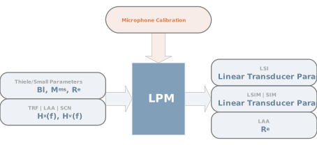
Malfunctions and Troubleshooting

Overview

This chapter will provide information that can help you solve common problems that occur with the Klippel Analyzer and the LPM module. The software generates a variety of warnings automatically if the signals are badly conditioned or a malfunction is detected. Some warnings may be neglected but it is always recommended to find out the cause of the problem.

If you cannot find a description here that matches your problem, check the Malfunction and Troubleshooting section in dB-Lab documentation or contact KLIPPEL support.

Error and Warning Messages

Primary data is already available

Measurement results will be deleted if the corresponding setup parameter are changed. This way, results and setup parameters are kept consistent. If you want to perform a new measurement while preserving the old results, please create a new operation. The setup parameters of the old measurement can be conveniently copied to a new operation with the Copy and Paste buttons that you find on property page Im/Export (see above). Furthermore, you can save the setup of the operation as Template for new operations.

WARNING: Stimulus is applied to OUT 1

This warning will be generated if Voltage: at OUT 1 is selected in property page Stimulus. In this case, the specified stimulus voltage is the voltage at the output connector OUT 1 (and hence at the amplifier input). The level of the amplifier output signal can be considerably higher than the specified level and can possibly destroy your speaker!

No proper amplifier output

Cause

The LPM tests the amplifier before the main measurement. During this test the pass band gain is measured at 750 Hz. Furthermore, the amplifier is tested at all frequencies lower than 50 Hz to determine the high-pass filter decay at low frequencies. The error message is generated if the amplifier is switched off or if the test signal is not transmitted properly.

Remedy

Check the amplifier. Check the SNR of the test signal (750 Hz and all lines below 50 Hz) in result window U(f) Voltage Spectrum. The SNR should be at least 35 dB for the 750 Hz line. Increase the amplifier gain. Check the connection and the cables in the hardware setup. Is the amplifier input connected to OUT 1? Is speaker cable connected to the speaker connector that is selected in property page Input?

Desired excitation level cannot be realized

Cause

This error message is generated if the amplifier gain is too small to realize the desired excitation level.

Remedy

Increase the amplifier gain. Use an amplifier if you did not use one so far and switch to Voltage: at Speaker terminals in property page Stimulus. Decrease excitation level to the value shown in the message box.

Speaker not connected

Cause

If no current signal is measured at the Speaker 1 or Speaker 2 channels of the analyzer, this warning will be displayed.

Remedy

Open the result windows i(t) Current Waveform and I(f) Current Spectrum and confirm that there is no current signal. Ensure that the speaker is connected. Check the connections and the used speaker cable. Make sure that the DUT is not damaged! Increase the excitation level if it is low. For KA3, DA Rev. \(\geq\) 2.1, PM8 Rev \(\geq\) 2.0 check the fuses. The fuse holders can be opened at Speaker Card or at the back side of the device. See KLIPPEL Analyzer Hardware manual for more information.

Measurement of DC voice coil resistance Re is corrupted

Cause

The DC voice coil resistance \(R_{\text{e}}\) is measured at the two lowest frequency signal lines. The error message is generated if the resulting impedance at the two frequencies differs considerably. This may be caused by bad SNR or impact of the driver resonance (insufficient spectral distance).

Remedy

Increase excitation voltage or number of averages in property page Stimulus. Always select Voltage: at Speaker terminals in property page Stimulus. The low frequency decay of the amplifier’s high-pass filter will be measured and compensated (max. 27 dB) in this mode. Use a series resistor to increase signal to noise ratio (see section Series resistor). Check the result windows I(f) Current Spectrum and U(f) Voltage Spectrum. Are the low frequency lines properly available?

Specified series resistor resistance is greater than the measured DC impedance

Cause

The measured DC impedance comprises the series resistor and the DC voice coil resistance. Therefore, it can never be exceeded by the series resistor.

Remedy

Check the connected series resistor. Compare the resistance specified in property page Method with the impedance curve (result window Z(f) Impedance Magnitude) at low frequencies. You may measure the series resistor with the LPM before connecting it to a driver. In this case the \(R_{\text{e}}\) parameter will show the value of the series resistor.

No proper current signal

This message will be generated if the ratio signal to noise + distortion of the measured current signal is lower than 20 dB. This means that either the noise is high and will corrupt the results or that there are more than 10 % distortions indicating that the small signal domain is already left. Please check the result windows i(t) Current Waveform and I(f) Current Spectrum to see the waveform and spectral content of this signal. There are some causes for the problem:

Cause

The amplitude of the measured current is too low.

Remedy

Increase the voltage of the excitation signal or the number of averaging in the property page Stimulus.

Cause

The signal to noise ratio at the resonance dip of the current spectrum is poor. This may occur if the driver has a very sharp resonance peak.

Remedy

Use a series resistor (see section Use a series resistor to increase signal to noise ratio above). Increase the voltage of the excitation signal or the number of averaging in the property page Stimulus.

Cause

The input current at the speaker terminals is distorted by the speaker’s nonlinearities. High amount of distortion in the current indicates that the linear model is not adequate anymore.

Remedy

Reduce the voltage of the excitation signal in the property page Stimulus. You may also ignore this warning.

Cause

There is a humming component in the excitation signal due to a ground loop. You may see the component in the result window I(f) Current Spectrum or in Table Signal Characteristics under I SNR+D and fi noise.

Remedy

Check your setup carefully.

Note

Increasing the number of averaging in property page Stimulus will not reduce distortion or a humming component.

No proper voltage signal

This message will be generated if the ratio signal to noise + distortion of the measured voltage is lower than 20 dB. This indicates that the amplifier produces significant noise or distortions (for instance caused by limiting). Please check the result windows u(t) Voltage Waveform and U(f) Voltage Spectrum to inspect the waveform and spectral content of this signal. There are some causes for this:

Cause

The amplitude of the measured voltage is too low.

Remedy

In this case please increase the amplitude of the excitation signal or the number of averaging in property page Stimulus.

Cause

The voltage at the speaker terminals is distorted by amplifier nonlinearities (limiting?).

Remedy

Reduce the amplitude of the excitation signal in the property page Stimulus.

Cause

There is a humming component in the excitation signal due to a ground loop. You may see the component in the result window U(f) Voltage  Spectrum or in Table Signal Characteristics under U SNR+D and fu noise.

Remedy

Check your setup carefully.

Remedy

If using a KA3 check if the force and sense lines are connected to the speaker clamps.

Note

Increasing the number of averaging in the property page Stimulus will not reduce the amount of distortion or a humming component.

Laser signal invalid

This message will be generated if there are less than five proper signal lines in the displacement spectra or if the strongest signal line is not at least 20 dB above the strongest noise component. Please check the result windows x(t) Displacement Waveform and X(f) Displacement Spectrum to see the waveform and spectral content of this signal. There are a few possible root causes for this error:

Cause

The distance between laser head and driver is not properly adjusted.

Remedy

See section Tips for Laser Usage in the Hardware Manual.

Cause

The laser head is not properly connected to the laser controller or the laser controller is not properly connected to the connector laser input of the analyzer.

Remedy

Please check the connections.

Cause

The amplitude of the measured displacement is too low. That might be caused by a high resonance frequency of the driver that is too close to the cut-off frequency of the laser head.

Remedy

In this case please increase the amplitude of the excitation signal or the number of averaging in the property page Stimulus.

Cause

The voice coil displacement is distorted by the speaker’s nonlinearities. High amount of distortion in the displacement indicates that the linear model is not adequate anymore.

Remedy

You may ignore this warning or reduce the amplitude of the excitation signal in the property page Stimulus.

Cause

The output of the sensor is distorted due to nonlinearities inherent in the triangulation principle used in the laser head.

Remedy

You may ignore this warning or increase the amplitude of the excitation signal in the property page Stimulus.

Cause

There is a humming component in the excitation signal due to a ground loop. You may see the component in the result window X(f) Displacement Spectrum.

Remedy

Check your hardware setup carefully.

Cause

There is dominant low-frequency disturbance (bump) in the noise floor of the X(f) Displacement Spectrum.

Remedy

This may be caused by settling effects of the DUT, laser mounting, after switching or by low frequency vibration that couples into your test setup.

Cause

The displacement spectrum will decay with 12 dB above the resonance frequency of the laser.

Remedy

The frequency fx cutoff where it disappears in the noise should be at least 300 Hz. You can check fx cutoff in Table Signal Characteristics. If there are no signal lines at all check the hardware connections.

Note

Increasing the number of averaging in the property page Stimulus will not reduce the amount of distortion or a humming component.

No proper laser signal

This message will be generated if the signal to noise + distortion ratio (\(X_{\text{SNR+D}}\)) is lower than 20 dB for one or more signal lines. Signal lines with a level less than 3 dB below the maximum level of the spectrum are ignored.

The message indicates that either the noise is corrupting the result or that there are more than 10 % distortions. In the latter case the small signal domain is already left. Please check the result windows x(t) Displacement Waveform and X(f) Displacement Spectrum to see the waveform and spectral content of this signal. There are some causes for the problem:

Cause

The level of the measured displacement is too low.

Remedy

Increase the voltage of the excitation signal or the number of averaging in the property page Stimulus.

Cause

The displacement is distorted by the speaker’s nonlinearities. High amount of distortion in the current indicates that the linear model is not adequate anymore.

Remedy

Reduce the voltage of the excitation signal in the property page Stimulus. You may also ignore this warning.

Note

Increasing the number of averaging in property page Stimulus will not reduce the amount of distortion.

Voltage sensor is limiting

The voltage sensor is limiting. Decrease stimulus voltage. Check voltage signal waveform and spectrum (result windows u(t) Voltage Waveform and U(f) Voltage Spectrum). Check your analyzer’s specification for absolute maximum values.

Current sensor is limiting

The current sensor is limiting. Decrease stimulus voltage. Check current signal waveform and spectrum (result windows i(t) Current Waveform and I(f) Current Spectrum). Check specification of hardware for absolute maximum values.

Microphone signal is limiting

The microphone signal measured at input IN 1 is limiting. Check your microphone and preamp. Check microphone signal waveform and spectrum (result windows p(t) Sound Pressure Waveform and p(f) Sound Pressure Spectrum). Insert an attenuator for decreasing the input level.

High Sensitivity current sensor selected

Warning

High Sensitivity current sensor selected: Voltage at the DUT (speaker) could be lower than specified, due to the used shunt resistor.

The current sensing shunt resistor used to get the best possible SNR in the current signal is placed in series to the DUT. Depending on the DUT’s impedance the shunt resistor causes a frequency depending voltage reduction at the DUT. The influence of the shunt resistor can be seen in the U(f) Voltage Spectrum and read in the Table Signal Characteristics which shows the measured voltage at the DUT in comparison to the specified voltage in the property page Stimulus.

This warning can be ignored in LPM used for small signal measurements, as the correct voltage measured at the DUT’s terminals will be used for all calculations.

Note

This warning is related to KA3 hardware. For High Sensitivity modified DA2, it will not be displayed.

Further Problems

Some Thiele-Small parameters are zero

If \(F_{\text{max}}\) and the relative resolution are not selected properly in property page Stimulus than the identification algorithm may fails and one or more Thiele-Small parameters are set to zero. The same effect can be caused by poor measurement signals. The identification algorithm aborts if the driver resonance frequency is less than 10 Hz and higher than \(\frac{F_{\text{max}}}{4}\). Please follow the instructions given in section How to Get the Best Performance? in part 3 of the Tutorial.

Driver resonance was not fitted

See section Some Thiele-Small parameters are zero.

No “Fitted” curves are displayed

No Fitted curves are displayed for the Electrical Impedance \(Z(f)\) and Transfer Function \(H_{\mathrm{x}}(f)\). Also the Thiele-Small parameters will be zero.

See section Some Thiele-Small parameters are zero.

Check the \(Z(f)\) Impedance Phase result window. A phase starting around -180°, not around 0° as expected caused the fitting algorithm to fail. In this case check your speaker cables, inverted SENSE wires could cause this effect. Although with the color coded red and black connectors for the positive and negative FORCE and SENSE wires this should be avoided.

See KLIPPEL Analyzer Hardware for correct speaker connection.