Utilities#
Overview#
The Klippel Analyzer system provides several tools free of charge. They are intended to provide versatile functionality, used to
perform different kinds of post processing,
help to automate and control complex measurement tasks,
offer access to external programs,
interact with the user in test sequences,
listen to (and export) waveforms of dB-Lab modules to improve root-cause analysis,
check the sensors of your measurement device,
manually operate the measurement system as a sinusoidal frequency generator,
…
ECM - Extended Creep Modeling#
Overview#
The Extended Creep Modeling (ECM) tool is an addition to the LPM – Linear Parameter Measurement. It estimates the linear transducer parameters using improved fitting algorithms, as well as two additional models to identify the creep effect of the suspension.
ECM is a post-processing tool, using the measured data of an LPM operation.
Background#
Note
The background theory of the available creep models is available in greater detail in the MMT – Multipoint Measurement Tool manual.
The traditional Thiele Small Loudspeaker Model considers the compliance of the suspension (Cms) and the mechanical losses (Rms) constant parameters. Taking the creep effect of the suspension into account, these parameters become frequency dependent.
The current Klippel LPM module (version 212) offers a creep model with a frequency dependent compliance increasing towards lower frequencies, but still constant losses:
This simple model delivers good results for speakers with low creep effect, but yields fitting results of limited accuracy for speakers with a high creep effect.
Knudsen Creep Model#
Knudsen proposed a model for the suspension creep [2] using a logarithm weighted with the creep factor λ:
This model is purely mathematical, based on the experience that the creep increases nearly linear towards lower frequencies, when viewed on a semi-logarithmic scale.
The parameter C0 contains the value of the real part at the resonance frequency fs but is not equal to the value of the compliance Cms(fs).
Ritter Creep Model#
A three-parameter model based on retardation spectra was introduced by Ritter [3].
Instead of becoming negative towards high frequencies the creep reaches a minimum compliance, which is described by C0. The frequency fmin corresponds to the minimum retardation time of the retardation spectra and can be interpreted as the frequency where the creep of the suspension starts to rise.
Requirements#
The tool performs post-processing on measured LPM data to estimate the linear parameters, including the electrical impedance (\(Z\left( f \right) = \frac{U\left( f \right)}{I\left( f \right)}\)) and the transfer function (\(H_{x}\left( f \right) = \frac{X\left( f \right)}{U\left( f \right)}\)) of the transducer.
Note
It is recommended to use vacuum measurements, hence a joined air volume would distort the estimation of the parameters of the creep model.
Property Page#
After creating a new ECM operation, you can open the property page to customize the setup.
Input#
- Select Operation - LPM Operation Name
Operation used for post-processing, set via dialogue or directly by name.
- Import Re
Electrical voice coil resistance at DC, importing this value will influence the fitting of all parameters.
- Calibrate Hx(f) with Force Factor (Bl) [1]
Calibrates the absolute value of the measured transfer function.
- Calibrate Hx(f) with Mass (Mms) [1]
Mass of the suspension, calibrates the absolute value of the measured transfer function.
Model#
- Measurement
Affect the names and exported parameters. See Application Note 49 for further information about this issue.
- Inductance Model
Inductance model used for the post processing. Available values:
none: consider the inductance as a constant parameter Le
LR2: shunted inductor model
Leach: two parameter model by Leach
Wright: four parameter model by Wright
- Creep Model
Models the creep effect of the transducer at low frequencies. Available models:
none: compliance is real and constant
Log: simple, real logarithmic creep model
Knudsen: complex logarithmic creep model by Knudsen
Ritter: complex creep model by Ritter
Result Windows#
Linear Parameter#
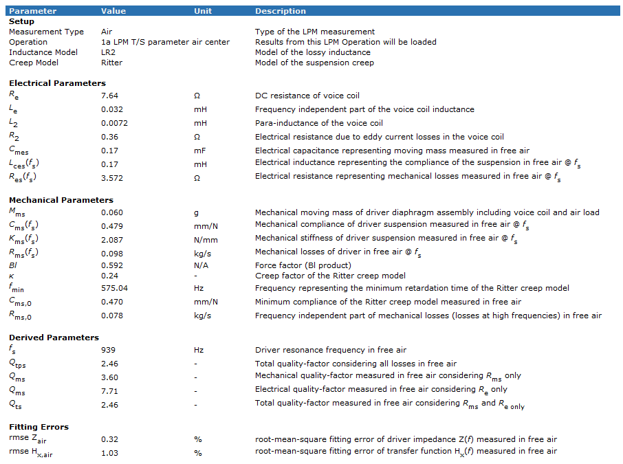
Shows the fitted parameters, as well as warnings, errors and other status messages.
Electrical Impedance Magnitude#
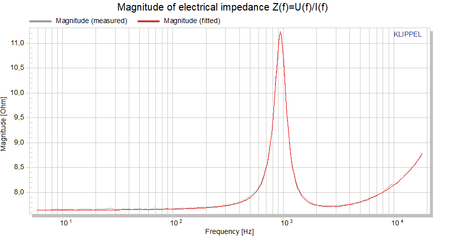
Displays the magnitude of electrical impedance |Z(f)| over the frequency f. There are no differences compared to the results in the LPM module.
Electrical Impedance Phase#
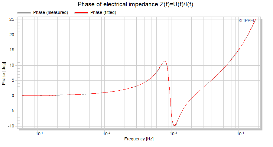
Displays the phase of the electrical impedance arg(Z(f)) over the frequency f. There are no differences compared to the results in the LPM module.
Hx(f) Magnitude#
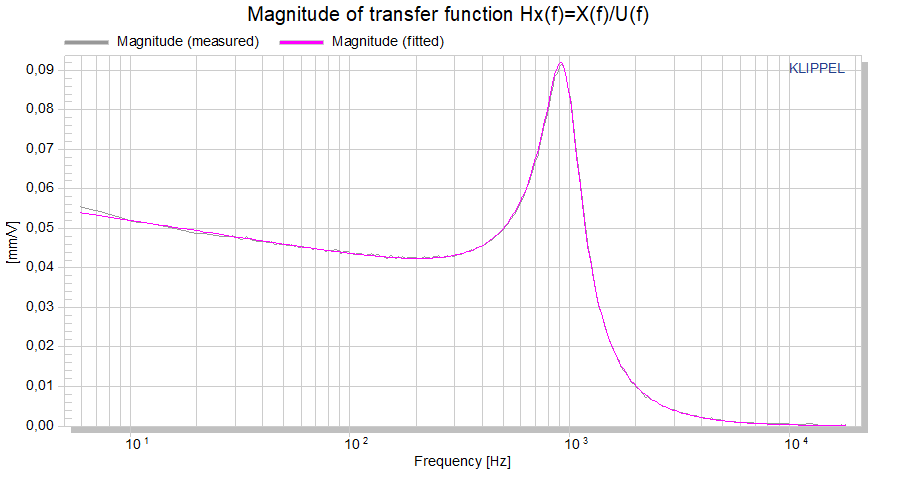
Displays the magnitude of the transfer function |Hx(f)| over frequency f. Importing a calibration factor (Mms or Bl) will shift the measured curve and mark it as imported.
Mechanical Impedance Magnitude#
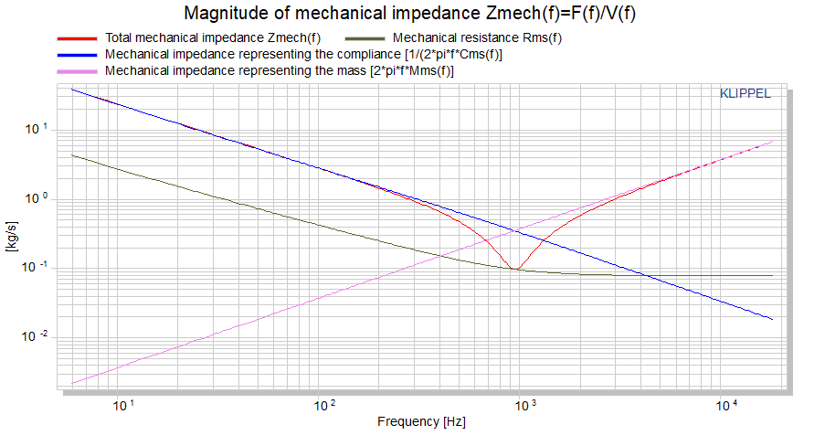
Displays the impedance magnitude of the mechanical components |Rms(f)|, |Cms(f)| and |Mms(f)|, as well as the magnitude of the total mechanical impedance |Zmech(f)| over frequency f.
Inductance Magnitude#
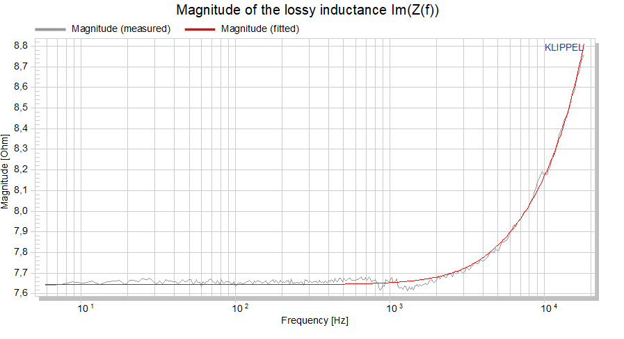
Displays the magnitude of the lossy inductance \(\left| \mathfrak{I}\left\{ Z\left( f \right) \right\} \right|\) over frequency f.
Inductance Phase#
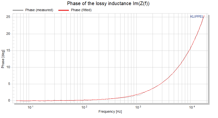
Displays the phase of the lossy inductance \(\text{arg}\left( \mathfrak{I}\left\{ Z\left( f \right) \right\} \right)\) over frequency f.
Mechanical Compliance#
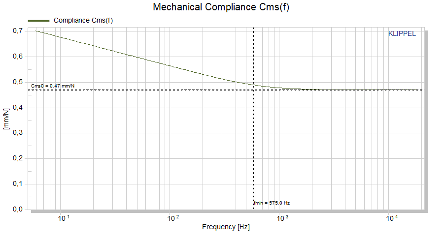
Displays the magnitude of the mechanical compliance |Cms(f)| over the frequency f. Linear value Cms0 and cutoff frequency fmin are marked, depending on the used model.
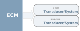
Supported Modules for Im/Export#
References#
W. Klippel and U. Seidel, “Fast and Accurate Measurement of Linear Transducer Parameters,” presented at the 110th Convention of the Audio Engineering Society, Amsterdam, May 12-15, 2001, preprint 5308
M.H. Knudsen and J.G. Jensen, “Low-Frequency Loudspeaker Models that Include Suspension Creep,” J. Audio Eng. Soc., vol. 41, pp. 3-18, (Jan./Feb. 1993)
F. Agerkvist and T. Ritter, “Modelling Viscoelasticity of Loudspeaker Suspensions using Retardation Spectra,” presented at the 129th Convention of the Audio Engineering Society, San Francisco, November 4-7, 2010, preprint 8217
K. Thorborg, A. Unruh and C. Struck, “An Improved Electrical Equivalent Circuit Model for Dynamic Moving Coil Transducers”, presented at the 122nd Convention of the Audio Engineering Society, Vienna – Austria, May 5-8, 2007
K. Thorborg, C. Tinggaard, F. Agerkvist and C. Futtrup, “Frequency Dependence of Damping and Compliance in Loudspeaker Suspensions”, J. Audio Eng. Soc. Vol. 58 no. 6, June 2010.
K. Thorborg and C. Futtrup, “Electro-Dynamic Transducer Model Incorporating Semi-Inductance and Means for Shorting AC-Magnetization”, J. Audio Engineering Society, vol.59 September 2011.
IO - Input Output#
The Input Output (IO) module is a tool for batch processing and controlling external periphery from dB-Lab. It can control Multiplexer, the MegaSig U980 Bluetooth® interface and can send and read commands via the GPIO of the KA3 hardware. In addition, the module can pause a batch run, wait for user interaction and run an external file.
Bluetooth®#
For measuring sound devices with Bluetooth® wireless technology the IO-Module is supporting a professional Bluetooth® interface: the MegaSig U980.
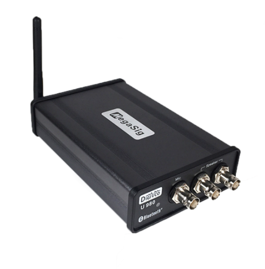
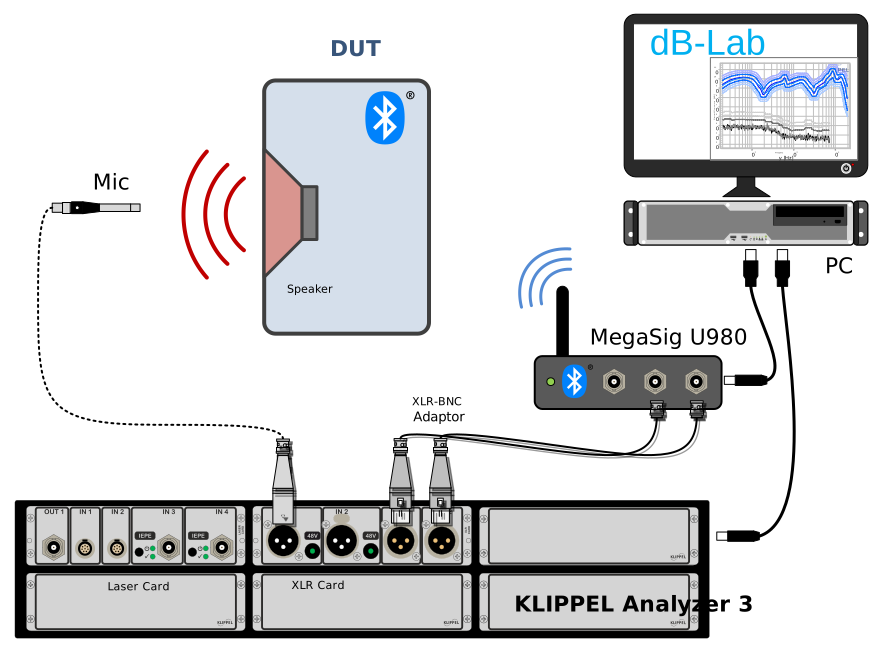
The scheme below shows a typical setup for a Bluetooth enabled stereo speaker. The MegaSig U980 contains two input channels for right and left channels labelled with Speaker and an output labelled with Mic for sending back a microphone signal. The output channel is not needed for loudspeaker measurements.
Parameter#
Settings#
The Settings section specifies the configuration of the Bluetooth interface.
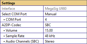
Select COM-Port#
Virtual serial port selection of Bluetooth interface. The port can be detected automatically or selected manually:
Automatic: COM-ports are scanned and the interface is selected automatically
Manual: with this option a specific COM-Port can be selected
A2DP Codec#
Using the A2DP audio profile, the Bluetooth® interface give several control parameter to perform measurement with specific Bluetooth® settings
- Codec
The U980 supports the following codecs:
SBC
aptX
aptX Low Latency
aptX-HD
If no codec is selected the interface will automatically choose a codec.
- Volume
Parameter to set the volume of the audio device.
- Sample Rate
- \(fs\) in \(Hz\)
Parameter to the set a specific sample rate. If this parameter is not defined the sample rate is set automatically.
- Audio Channel (SBC)
Using the SBC codec the audio channel can be also controlled. There are the following options available:
Joint Stereo
Stereo
Dual Channel
Mono
If no specific channel setup is selected this will be set automatically.
Pairing#
The IO-module can pair automatically or to a specific device by defining the name or Bluetooth® address of the device.
- Automatic Pairing
If the paring is set to automatic the interface will connect to the next available Bluetooth® device.
- Pairing by Friendly Name
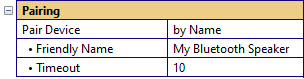
The interface will pair with the next device that matches the defined friendly name. Also substrings are supported.
- Pairing by Bluetooth Address
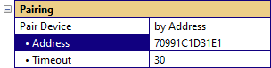
The interface will pair with the next device that matches the Bluetooth® Address.
- Select Device
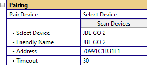
In this mode the Interface can search for available Bluetooth® devices. All available devices will be listed and can be selected for a controlled pairing.
- Timeout
- in \(s\)
Maximum time span for scanning and pairing.
Profiles#
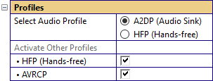
Selection of the Bluetooth profiles.
- Audio Profile
Parameter specifies the Bluetooth audio profiles. The following profiles are provided:
A2DP
HFP
- Activate Other Profiles
In addition to the audio profile also other profiles, which are not used for the audio streaming, can be activated. The following profiles are provided:
A2DP
HFP
AVRCP
Results#
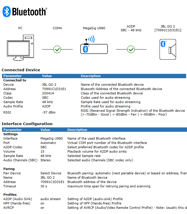
The Bluetooth® result window summarizes the information of the Bluetooth® interface. It shows an overview as well as the specific setting of the interface (e.g. codec, sample rate, COM-Port, etc.) and properties of the connected audio device (e.g. Bluetooth® address, RSSI, class, etc.)
GPIO#
The KLIPPEL Analyzer 3 has a GPIO to send or receive command. The IO module can set and read the configuration of the GPIO to interact with external hardware during a measurement sequence (batch run).
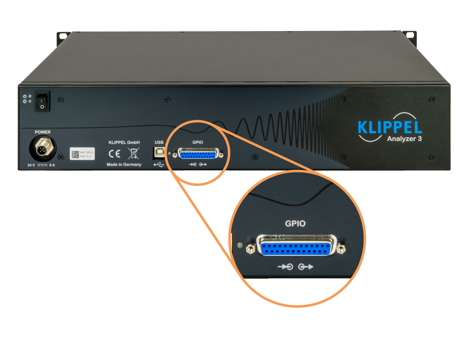
For further detail about the electrical characteristics please see the KA3 Specification H3.
Parameter#
Operation Mode#
The IO module can be either used to set outputs of the GPIO or to read the inputs. In the following the different mode are described in detail.

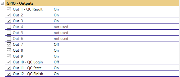
Switch - Single Command#
This mode can switch all 12 GPIO outputs to a specific configuration. Each channel can be either switched on, switch off or can be ignored.
Switch – Sequence#
This mode can send complex switching pattern via the outputs. For each channel an individual switching sequence can be defined by specifying a time curve. The first column is the time in seconds and the second column the switch state. (0=off/ 1=on).
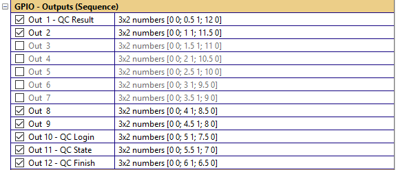
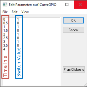
For example, the module can generate a pulse that is use to control a 3rd party multiplexer.

Note
Timing of the sequential switching isn’t very accurate and has a minimum resolution of 100ms. It has a high jitter and is not suitable to be used as an accurate clock-pulse generator.
Input Trigger/ Polling#
The IO module can also read all 8 GPIO input simultaneously. It can be operated in 2 modes, as a trigger or in a continuous monitoring (Polling) mode.
In the Input Trigger mode, the IO module stays in a loop until the GPIO input matches the required configuration. For example, this can be used in a power test application. So the batch run can pause until certain temperature is reached. Analogous to the output configuration also the Inputs can be either on, off or not considered.
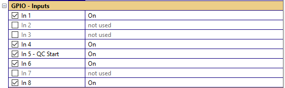
The Input Polling is a continuous measurement mode, which can monitor all 8 Input channel in real time.
The update cycle of the input channels is relatively slow (>100ms) and short impulses may not be detected.
Display#
Using the Display section, input and outputs that are not used can be hidden.

Results#
GPIO Configuration#
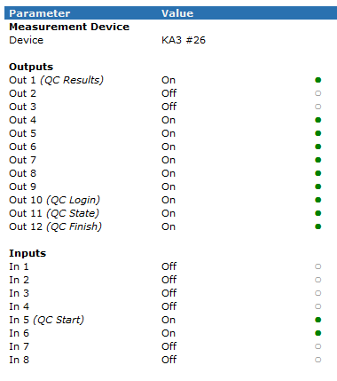
The window summarizes the last state of the GPIO configuration.
GPIO Output#
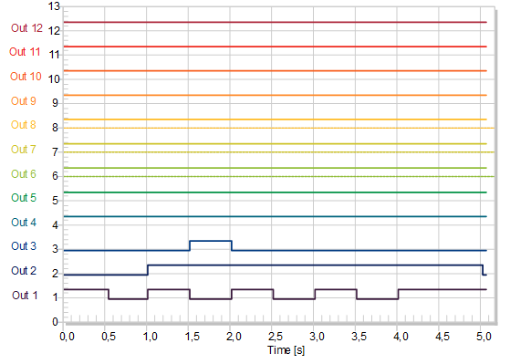
The GPIO Outputs window visualizes the setting of all 12 outputs over time.
GPIO Inputs#
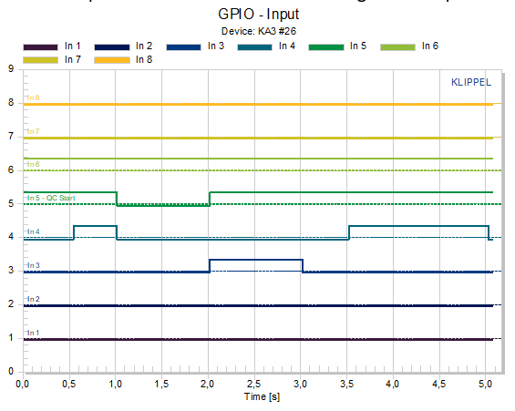
The GPIO Inputs window visualizes the setting of all 8 inputs over time.
Multiplexer#
Parameter#
Device#
- ParameterName
In the device category the used multiplexer can be selected. The following option are provided:
Automatic: The first device that is found will be switched
All: All connected multiplexer will be switched
Serial Number:The multiplexer with the specified serial number is switched (multiple devices can be specified)

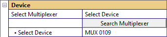
Select Device: In this mode the module can search for available multiplexers. All available devices will be listed and can be selected.
Routing#
- Mode
The Klippel Multiplexer have several switching modes which are defined in the following:
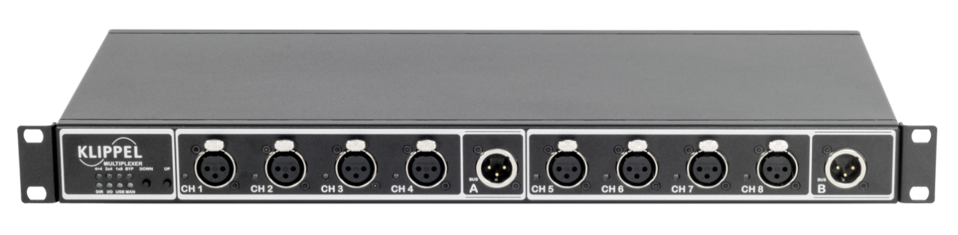
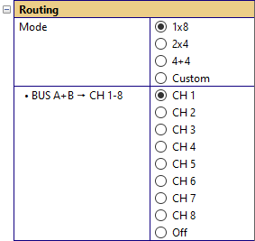
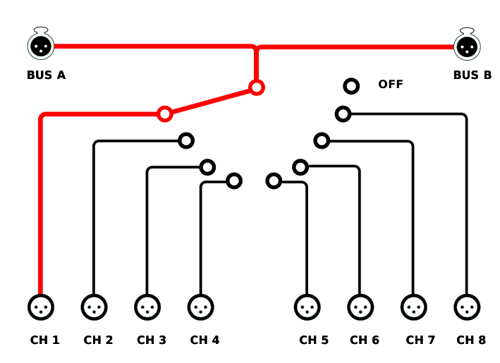
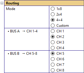
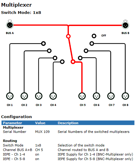
1x8 – Single (1 out of 8): The 1x8 Mode select 1 of the 8 channels. Both BUS connectors are bridged.
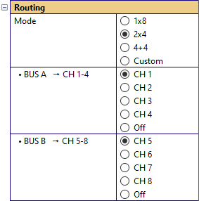
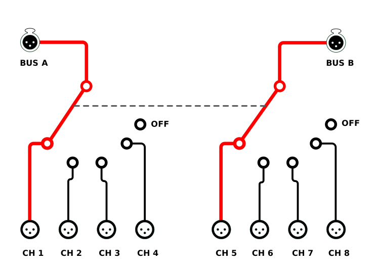
2x4 – Dual Parallel (2 Out of 4): The 2x4 Mode switched BUS A and BUS B in parallel.
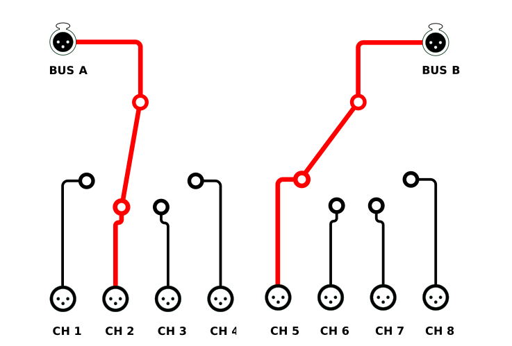
4+4 – Dual Separate (1 out of 4): The 4 +4 mode gives separate control of the BUS connectors.
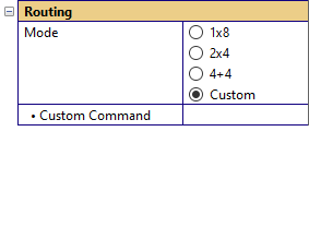
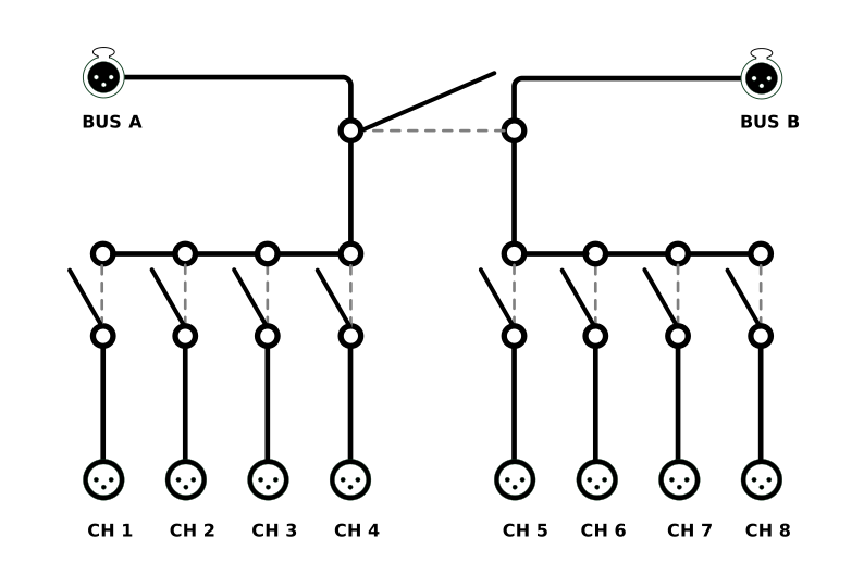
Custom: In the Custom mode the IO-Module can send a list of commands to the multiplexer. The Hardware can be set to any possible combination of the internal relays. Therefor the following comands are available:
'custommode on'   //switches on the code mode
'custommode off'  //switches off the code mode
'set1x8 x'        //replace x with the desired channel number
'set2x8 x'        //replace x with the desired channel number
'setrelais x on'  //closes relais x
'setrelais x off' //open relais x
Note
The command needs to be framed by inverted comma. Apostrophes are not allowed. Switching on the custommode is required. Before using one of the other modes, the custommode has to be switched off again.
- IEPE Supply (BNC-Multiplexers only)
Using a BNC-Multiplexer, the device can supply IEPE –Power to the connected microphones. This can be activated using the parameters Set IEPE – CH 1-4 and Set IEPE – CH 5-8.

Results#
The switch configuration and a summary of the multiplexer settings is summarized in the multiplexer result window.
Pause#
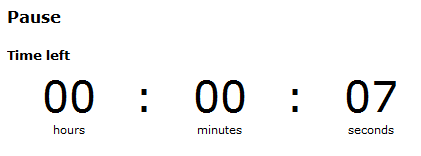
The IO-module has a pause option. This can be used to pause a batch run for a certain time e.g. for cooling down the speaker. The pause is specified in hours, minutes and seconds.

During the module is waiting the remaining time is shown in the Pause result window.
Message#
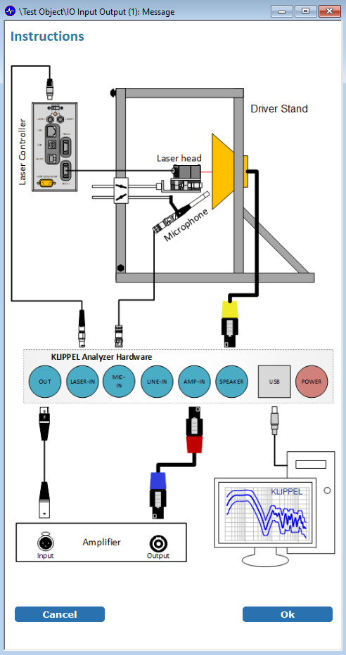
Message to stop a batch run and wait for a user interaction.
File Execution#
To trigger an external process the IO-module can execute a file e.g. a *.bat.
IMO - Input Monitoring#
Overview#
Using a KLIPPEL Analyzer 3 in combination with dB-Lab allows monitoring of the time signal and spectrum of one input signal. The Input Monitoring (IMO) tool allows the capturing of line signals (In1/In2), voltage and current, as well as displacement. A simplified long-term measurement, showing some statistical values of the captured signal (peak / bottom / mean / RMS), allow to see long changes over time.
Property Page#
Measurement Setup#
- Input
Defines the monitored signal. Available are:
In1 / In2 (line signals with optional microphone calibration)
Voltage/Current (at Speaker 1 or Speaker 2 channel)
X (displacement)
Route to Laser Card Output If checked, the monitored signal is routed to the output of the Laser Card. The transmission factor is shown when the monitoring runs.
The voltage at the Laser Card OUT1 connector is defined by the following formula:
\[U_{\text{OUT}1} = U_{\text{IN}}\cdot C_{\text{Laser Card Transmission}}\]Note
For measurements with external sensors (e.g. using a laser), the sensor calibration has to be considered additionally to calculate the absolute displacement out of the voltage at the Out1 connector.
- Sample Rate
- in \(\text{Hz}\)
Sample rate of the measurement. Note that the maximum available monitoring time depends on this value.
Available are:
48 kHz (Tcapture ≤ 20s)
96 kHz (Tcapture ≤ 10s)
192 kHz (Tcapture ≤ 5s)
- Capture Block Optimized for
Presets with optimized capture times depending on different measurement tasks. Available are:
Input Meter: Optimized for high performance
Frequency Resolution: Optimized for a good frequency resolution (1 Hz)
Custom: Length defined by the user in either seconds or samples. Note that the maximum monitoring time depends on the sample rate.
Sensor Configuration#
- Type
Type of the connected sensor. Depends on the chosen Input:
IN1/IN2: Managed by dB‑Lab, Microphone, Acceleration Sensor.
X: Laser, B‑Field Sensor.
Note
”Managed by dB‑Lab” means that the microphone configuration is handled by dB‑Lab. See dB-Lab – Software manual for more details.
- Sensitivity
- \(\text{mV/Pa, mV/m/s²}\)Range: \(> 0\)
Either sensitivity of a connected microphone, or acceleration sensor.
Measurement Control#
Only available during measurement.
- Freeze Instantaneous Monitoring
Stop updating of the windows Input Waveform and Input Spectrum, stopping at the last captured state. The window Input long‑term will be unaffected.
- Reset Sensor Zero Position
Reset the sensor position to zero. May help if the laser position was changed during measurement.
- Reset Data
Delete monitored data during measurement.
Display#
- Unit of X-Axis
Unit of the x-axis in time related windows. Available values:
time (s)
samples
- Long-term Memory Time
\(\text{s}\)
Number of seconds displayed in the window Input Signal (mean), before the data at the beginning is discarded
- Apply Window to Spectrum
If checked, the input spectrum is calculated with von Hann window applied.
Result Windows#
Input (long‑term)#
Shows statistical time signal measures. Data is stored according the setting Memory time in s.
Input Level long-term#
Shows the RMS value of the measured signal scaled to the respective reference value:
Voltage: uref = 1 V
Sound Pressure: p0 = 20 µPa
Displacement: xref = 1 mm
Input Waveform#
Shows the high-resolution time signal of the last measured signal block according to the setting Unit for X-Axis and Measurement length optimized for.
Input Spectrum#
Shows the frequency spectrum of the last measured signal block according to the setting Measurement length optimized for:
State#
Contains information about the setup and the input signal.
Input Signal#
- Measured Value
Depending on the chosen input signal, displays the RMS or mean value of the captured input signal.
- Peak
Accumulated peak value of the input signal since start of the operation / last use of Reset Data.
- Bottom
Accumulated bottom value of the input signal since start of the operation / last use of Reset Data.
- DC
Mean value between aforementioned peak and bottom value
\[\frac{Peak + Bottom}{2}\]- Peak to Peak
Difference between aforementioned peak and bottom value
\[Peak - Bottom\]
Setup#
- Input Signal
Chosen captured input signal.
- Sample Rate
- \(\text{Hz}\)Sample rate of the capture device
- Route to Laser Card OUT1
Shows if the captured signal is routed internally to laser card OUT1 for external connection.
Note: You’ll need to apply a transmission factor to the signal, see Route to Laser Card Output parameter description.
PLAY - Audio Player#
Overview#
Note
The PLAY module will soon be replaced by the TFA module. The TFA module incorporates all functionalities of the PLAY module. It is recommended to use the TFA module instead of the PLAY module.
The PLAY Audio Player tool allows to listen to wave-form signals captured in dB-Lab, imported via the Clipboard. It is able to play the whole signal and sections, as well as down sample the signal to identify e.g. Rub and Buzz effects in the residual signal of the TRF Transfer Function Pro.
You can export the down sampled file (whole waveform or just selection) to the HDD for later usage.
Property Page#
Input#
- Import from Clipboard
Import the curve from the clipboard which will be played.
Any Matlab conform curve input is supported. The curve has to be in column-major order.
A field Curve is expected to hold curve data. For matrices with more than two columns, second column is expected to hold the playback data.
- Sampling Frequency
- in \(\text{Hz}\)
Sampling frequency of the imported curve. If the curve is a curve from a dB-Lab window, sampling rate of the curve will be automatically determined and set.
Processing#
- Normalize Playback
Normalize waveform to maximum before playback / export.
- Playback Rate
Represents the “speed” of the playback. Factors smaller 1 will slow down the playback, factors greater 1 will speed up the playback.
Also affects the pitch (slow down: pitch down; speed up: pith up).
Export#
- Mode
Exported part of the signal. Down sampling and normalization is applied according to the setup.
Available values:
all: Export whole signal
selection: Export select part of the signal
- Path
File on the hard disk used to store the exported signal.
Result Windows#
Input Curve#
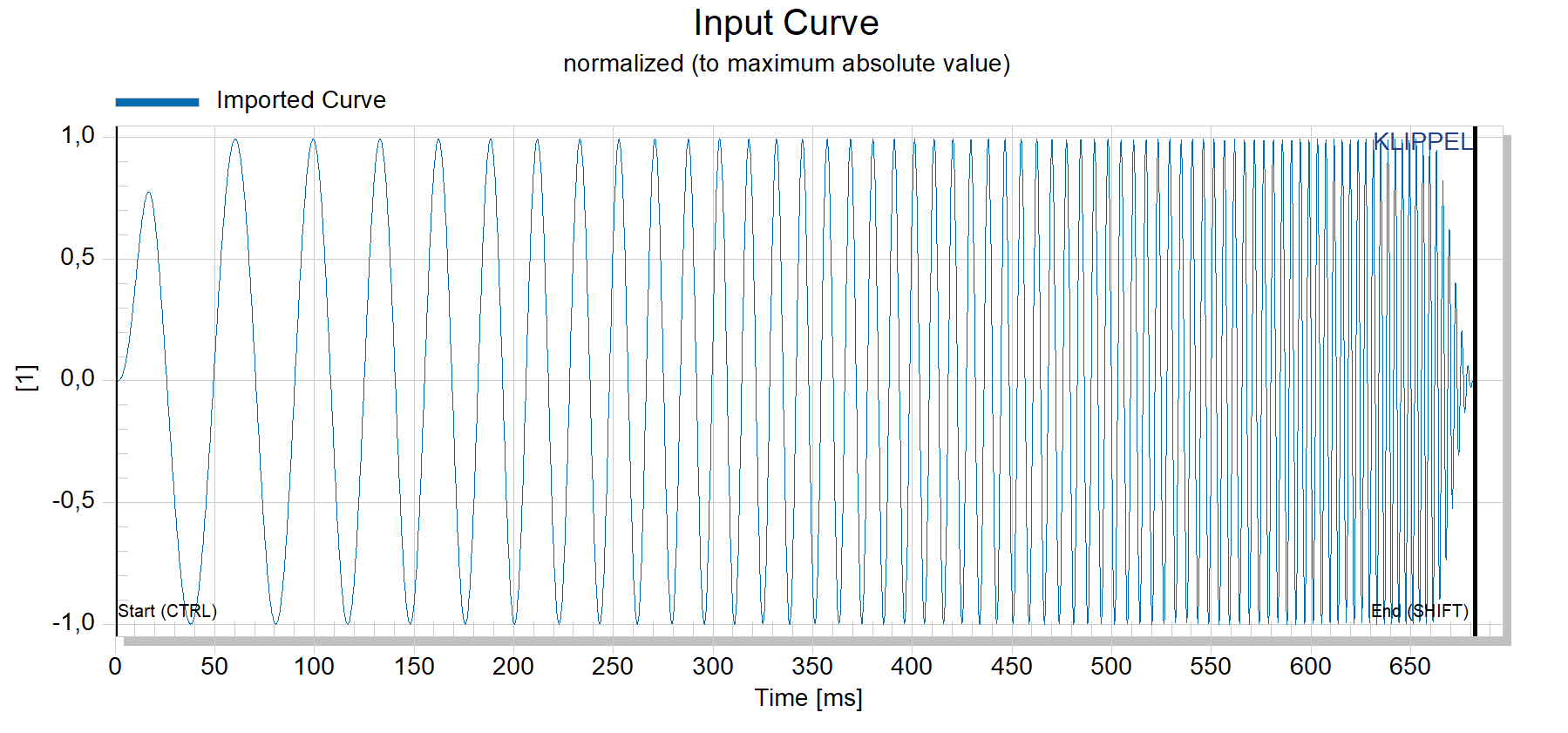
Shows the complete imported signal which can be used for playback. Using two cursors, the playback section can be defined. Use the cursors to specify a target play section. “Ctrl+LMB” (left mouse button) specifies the begin of the section, “Shift+RMB” (right mouse button) specifies the section which is played. Both cursors can also be moved using the mouse only.
Playback#
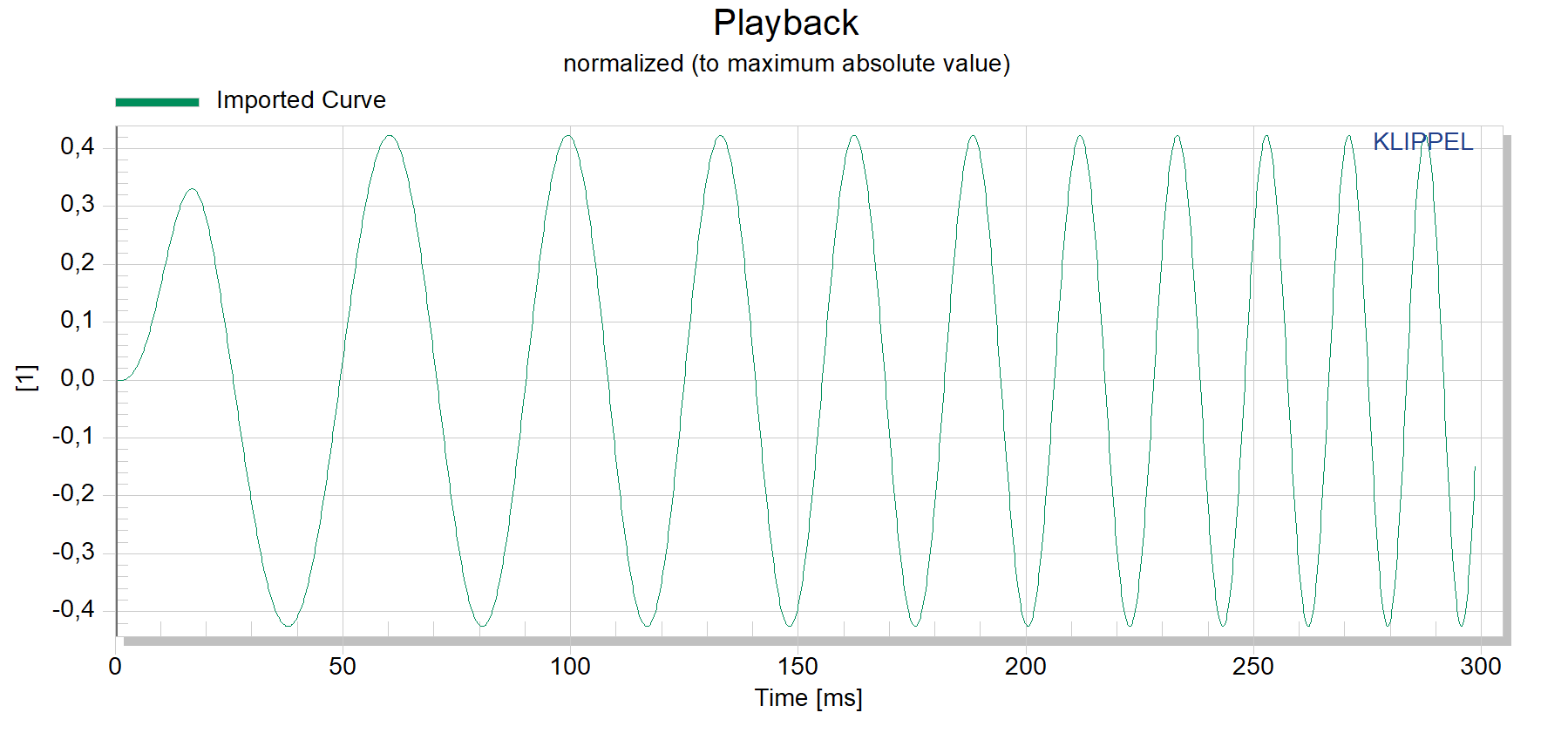
Shows the section specified by the cursors in the window Playback. This section will be played.
TRF Voltage Stepping#
Overview#
The TRF Voltage Stepping module is a tool to create an automatic test sequence with a systematic voltage increment. The basis can be any TRF – Transfer Function Measurement operation with arbitrary settings (e.g. signal routing, smoothing, harmonic and impulsive distortion analysis etc.)
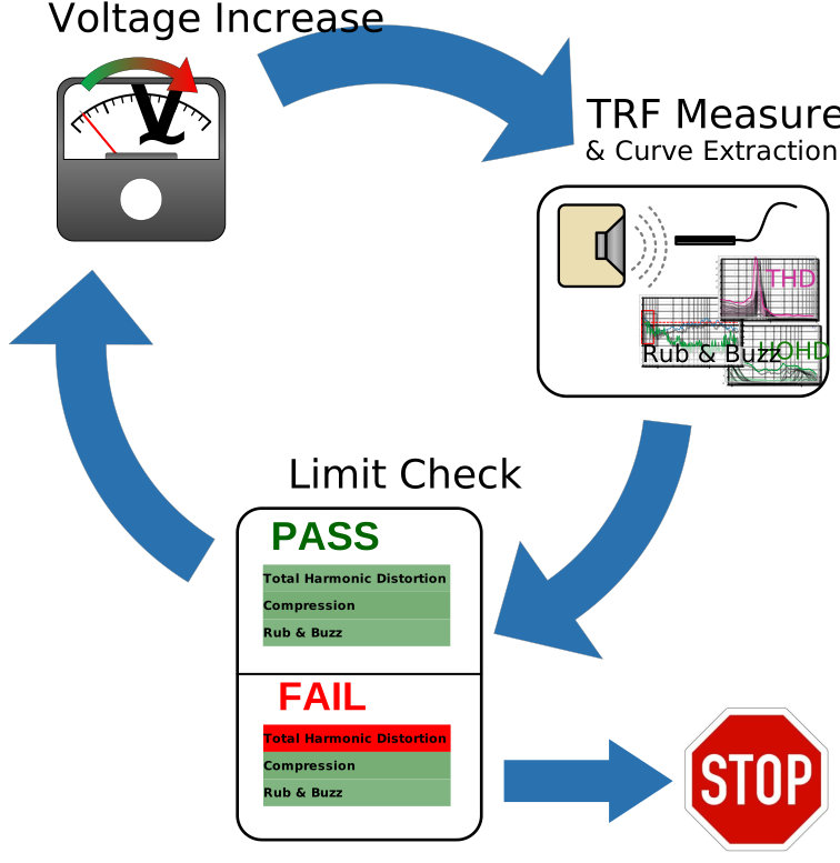
During the measurement the TRF Voltage Stepping is creating a batch of operation and increments the RMS input voltage of the measurement stimulus automatically. In addition, selected results such as harmonic distortion (THD, HOHD) are extracted from each measurement. Optionally, these results can be checked against limits to stop the measurement batch at a certain level e.g. when a defined level of THD is exceeded or a distinct Rub & Buzz is detected.
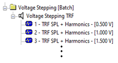
Once the measurement loop is finished, the Voltage Stepping module summarizes the extracted curves and all individual TRF measurements are stored in the database. Thus, critical measurements can be analyzed in detail.
Tutorial#
Viewing Result (Part 1)#
Open Measurement Example#
Open the Example Database and select the folder:\Frequency Response + Distortion (TRF, DIS, TBM, …)TRF Voltage Stepping (STEP)
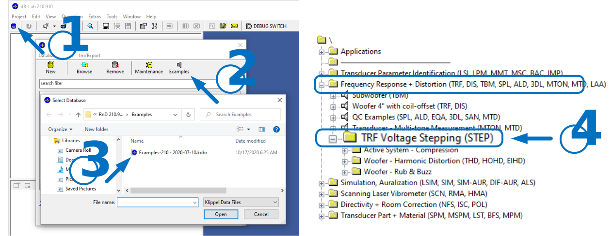
Select the folder Woofer - Harmonic Distortion (THD, HOHD, EIHD) and double click the operation STEP - Voltage Stepping TRF.
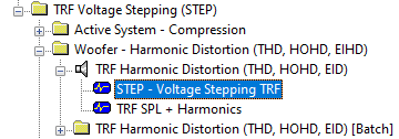
This example is showing a harmonic distortion measurement of 4” woofer. The TRF Voltage Stepping module was used to target a specified THD limit. The input voltage was increasing until a certain level of total harmonic distortion (THD) has been reached.
Measurement Operation and Voltage Definition#
Open the Properties Page, select the Setup Tab and expand the Input category.
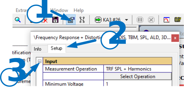
The Input category is defining the operation to perform the measurement as well as the input voltage that is applied to the device under test.
Most settings are configured in the TRF measurement operation (e.g. signal routing, frequency range, smoothing, etc.) The TRF Voltage Stepping module is only modifying the input voltage of the TRF operation and is creating a successive batch.
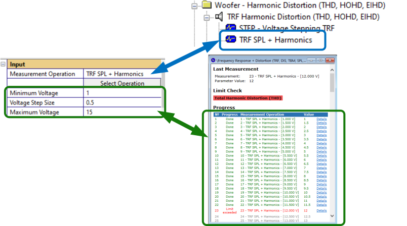
Results#
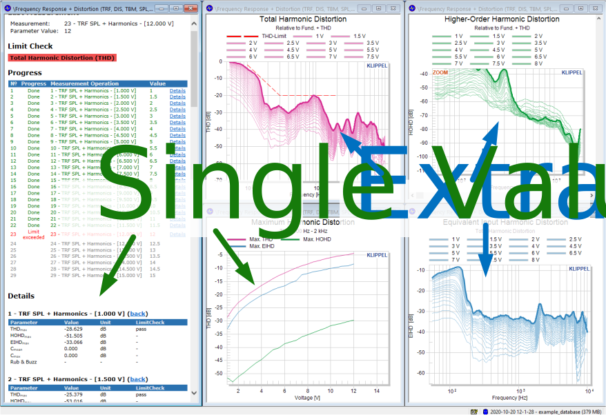
For each measurement a set of results will extracted and displayed in the TRF Voltage Stepping module. This includes curve results (e.g. THD, HOHD, compression) as well as single values displayed in the Details section of the Summary window. Other values are plotted over the input voltage (e.g. max. THD, Compression Peak and Mean).
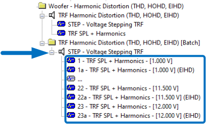
Furthermore, all individual TRF measurement operations are stored in an additional driver object, giving the complete set of data for a detailed analysis of critical measurements.
Limits#
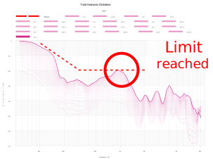
Optionally, TRF Voltage Stepping can apply limits to stop the measurement, for example when a certain level of distortion is reached. In this example a THD Limit was defined and at 12 Vrms the THD has reached 10% (-20dB) and the measurement batch was stopped.
THD Limit:
Freq. [Hz]    THD [%]

100             80
300             10
2000            10
Property Page#
Input#
- Measurement Operation
Name of the TRF operation that should be controlled by the TRF Voltage Stepping module. The operation must be in the same Driver Object.
- ParameterName
- \(symbol\) in \(unit\)Range: 20Hz .. 20kHz
- Voltage Definition
The TRF Voltage Stepping is increasing the input voltage linear using the following parameters.
- Minimum Voltage
- in \(\text{V}\)
Smallest voltage applied to device under test.
- Voltage Step Size
- in \(\text{V}\)
Voltage increment (linear stepping).
- Maximum Voltage
- in \(\text{V}\)
Maximum Voltage that will be applied to the device under test.
Processing#
The relative harmonic distortion measures (THD and HOHD) can be referenced to the following curves or values
Fundamental + THD
Fundamental
Mean sound pressure level in specified frequency band
- THD Reference
Reference Curve or Value for total harmonic distortion THD
- HOHD Reference
Reference Curve or Value for higher order harmonic distortion HOHD
Limits#
Limit Definition#
The TRF Voltage Stepping provides an automatic limit check of the extracted measurement of the performed TRF operation. Optionally, these limits can be used stop the measurement batch, e.g. at a certain level of harmonic distortion, compression or on detection of a Rub & Buzz defect.
Single Value Limit#
The simplest option to define a limit is a single value. For Example:
THD-Limit = 10 %
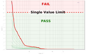
In that case the result curve is checked against this limit over the full frequency range. If the curve exceeds this limit at any point, the verdict is “FAIL”.
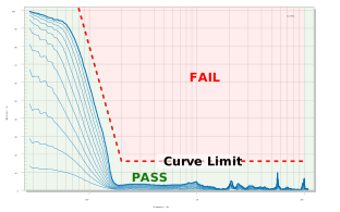
Curve Limit#
A limit can also be defined as a curve of frequency - value pairs. If the measure exceeds the limit curve in the defined range, the verdict is “FAIL”. For Example:
Freq. [Hz]      THD-Limit [%]

100                 80
200                 15
10000               15
Combined Rub & Buzz Limit#
To ensure a robust check of impulsive distortion, the Rub & Buzz Limit combines both IDR (Impulsive Distortion Ratio) and ICID.
The verdict is “FAIL”, when both ICID and IDR are above the critical threshold in the same frequency band. That means there is a distortion that is both impulsive and loud enough to be audible at the same time.
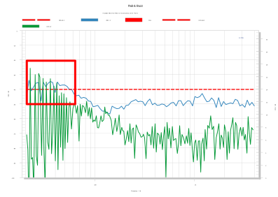
The Rub & Buzz Limit can be defined either as single values:
IDR [dB]      CID [dB]

-40           12
or as a curve:
Freq. [Hz]      IDR [dB]      CID [dB]

50              -40           14
200             -40           12
1000            -40           12
List of Parameters#
- Limit Exceeded
This Radio button controls if the measurement batch will be stopped when a limit is reached.
- THD
- in \(\text{%}\) or \(\text{Hz,%}\)
Maximum total harmonic distortion
- HOHD
- in \(\text{%}\) or \(\text{Hz,%}\)
Maximum higher order harmonic distortion
- EIHD
- in \(\text{%}\) or \(\text{Hz,%}\)
Maximum equivalent input harmonic distortion
- Max. Compression
- in \(\text{dB}\) or \(\text{Hz,dB}\)
Maximum compression of the transfer function
- Mean. Compression
- in \(\text{dB}\) or \(\text{Hz,dB}\)
Mean compression of the transfer function
- Rub & Buzz
- in: \(\text{IDR dB, ICID dB}\) or \(\text{Hz, IDR dB, ICID dB}\)
Combined limit of IDR and ICID.
Additional Operations#
Using the checkboxes in the category Additional Operation, the TRF Voltage Stepping module can create automatically new operations of the following types:
EIHD Equivalent Input Harm. Distortion
Time Frequency Analysis (TFA)
Audio Player (PLAY)
Especially for the detailed analysis of Rub & Buzz symptoms this is very useful. The additional operations are stored with the TRF operation in a folder in the database.
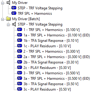
- EIHD Equivalent Input Harmonic Distortion
When this checkbox is activated, equivalent input distortion of each measurement are calculated automatically. Either the fundamental frequency response of each measurement or the transfer function of the first measurement can be used as the reference filter.
- TFA Time Frequency Analysis
This checkbox can be used to create automatically TFA operation of the individual TRF operations. This can be done for each measurement or only the last measurement.
Note
This feature requires a TFA Licence.
- PLAY Residuum
This checkbox can be used to create automatically PLAY operation of the individual TRF operations. This can be done for each measurement or only the last measurement.
Result Windows#
Summary#
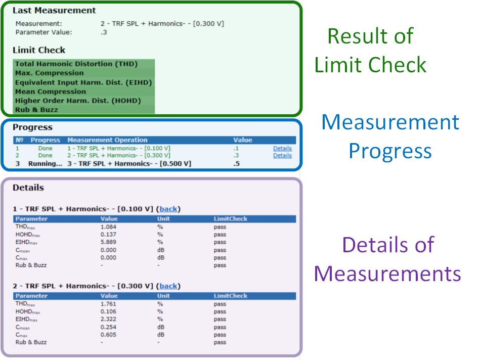
The Summary window displays the current state of the measurement. It shows the results of the limit check of the last measurement, the current position in the measurement batch and stores single value results of the individual measurements. Errors and warnings will be propagated to this window as well.
THD Total Harmonic Distortion#
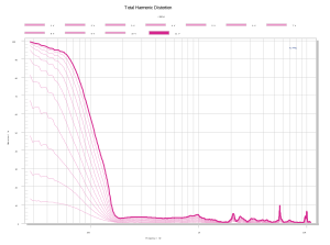
The graph shows the relative Total Harmonic Distortion of all individual measurements calculated from the RMS values of the n-th harmonic component according to IEC60268-21.
The sound pressure reference can be:
Fundamental + THD
Fundamental
Mean sound pressure level in specified frequency band
HOHD Higher Order Harmonic Distortion#
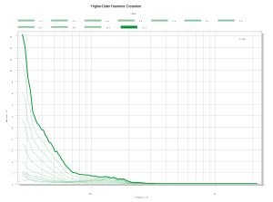
The graph shows the relative Higher Order Harmonic Distortion of all individual measurements calculated from selected higher order harmonic (Nl to N) components according to IEC60268-21.
The sound pressure reference can be:
Fundamental + THD
Fundamental
Mean sound pressure level in specified frequency band
EIHD Equivalent Input Harmonic Distortion#
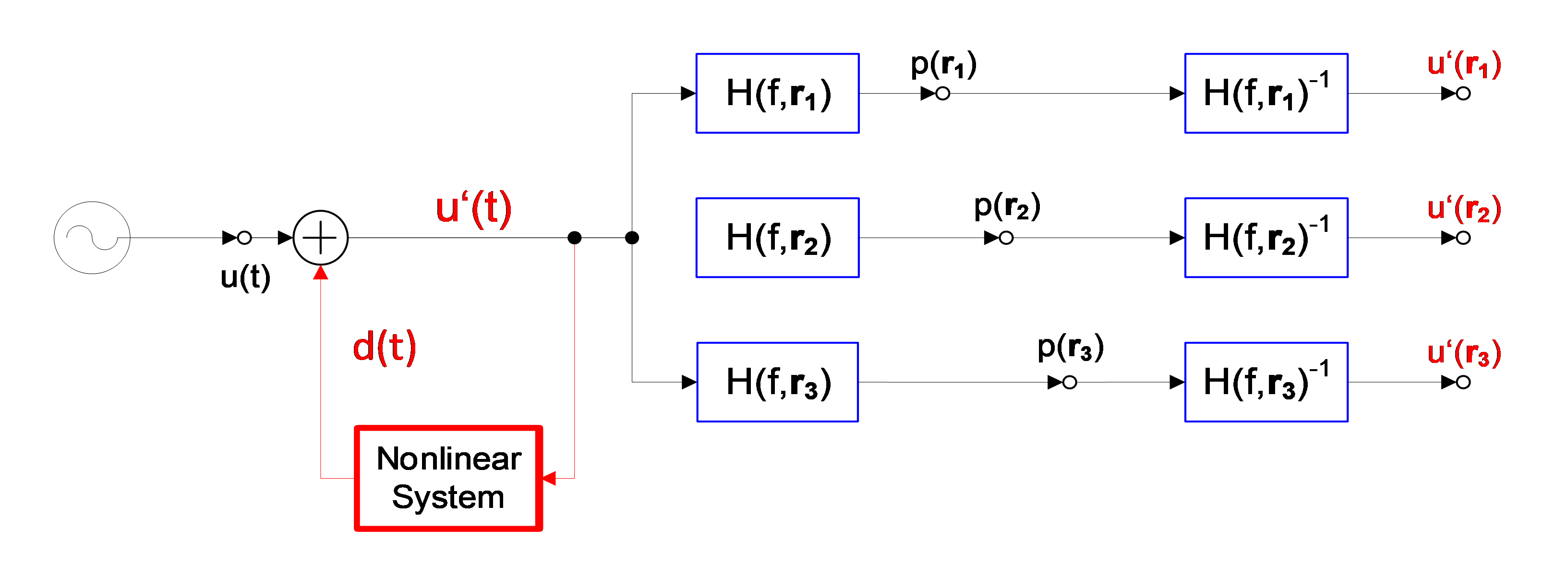
Harmonic distortion of loudspeakers is usually measured using a microphone at a certain position in the sound field. Thus, the distortion components are shaped by the fundamental frequency response and measurements at different positions may give totally different results.
By filtering the sound pressure with the inverse fundamental frequency response, the influence of the radiation can be removed and all distortion are transformed back to the input of the system. These so-called Equivalent Input Harmonic Distortion (EIHD) are very useful for comparing different measurements.
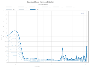
The Equivalent Input Harmonic Distortion are displayed vs. frequency and the maximum value is plotted in the specified range vs. voltage.
Max. Harmonic Distortion#
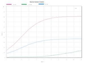
The window shows the maximum values of the harmonic distortion over the voltage steps. It includes total harmonics distortion THDmax(U), higher order harmonics distortion HOHDmax(U) and equivalent input harmonic distortion EIHDmax(U).
Compression#
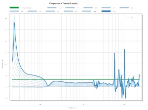
According to IEC60268-21 the time varying compression of the magnitude of the transfer function C(f,U) is calculated by the level difference of the transfer function H(f,u)compared to the linear transfer function Hlin(f,Ulin)at a certain reference voltage Ulin.
- C(f) Compression
- The C(f) Compression windows shows and compression of the transfer function over frequency and the mean compression calculated in a specified frequency band.
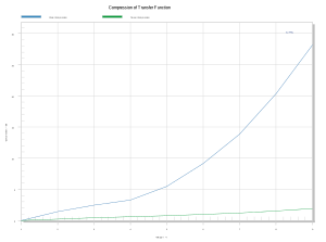
- C(U) Compression
- The C(U) Compression windows shows the maximum and mean compression values over the stepping voltage U.
Fundamental Mean#
This graphic window is showing the mean value of the fundamental frequency response over the voltage. The frequency range of the calculation is defined in the TRF measurement operation in Property page tab I-Dist.
Max. Impulsive Distortion Ratio#
The graph is visualizing the maximum impulsive distortion ratio over voltage. According to IEC60268-21 IDR is defined by:
Rub + Buzz#
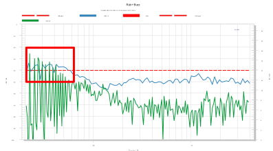
The Rub & Buzz graph contains the Instantaneous crest factor of the impulsive distortion ICID and the IDR according to IEC 60268-21.
Manual Sweep#
Overview#
The Manual Sweep is an easy to use sine sweep generator with a real time analyzer (RTA) included.
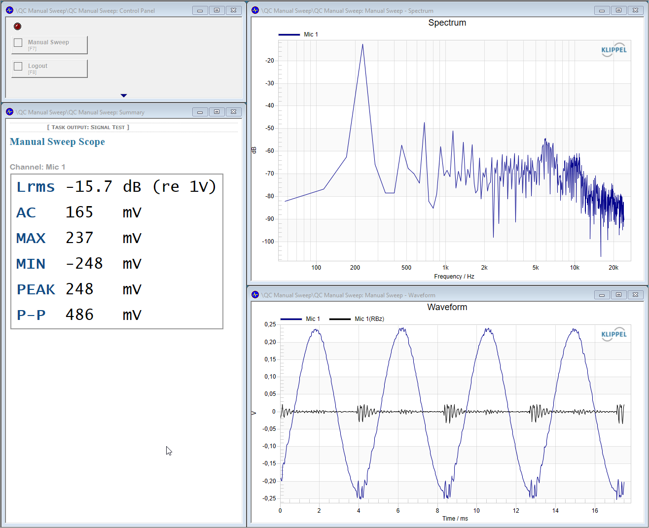
The result windows provide the spectrum and waveform data for the fundamental and also Rub & Buzz measures added by a table of single number results.
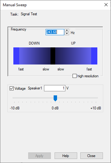
The Manual Sweep could be controlled by a SW interface for frequency and voltage control as well as by an optional hardware Manual Sweep Controller.
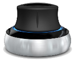
The Manual Sweep Controller requires a Klippel provided driver and settings package. It is available withing the dB-Lab software package. Any driver or SW from 3D CONNEXION, the manufacture of this 3D Mouse, is not required and should not be used as it could cause a deviating behavior.
As the Manual Sweep is a common QC tool it is descibed in further details in the QC manual at chapter Manual Sweep.
This Tools manual just highlightes the differences when it should be used within the R&D Framework.
The Manual Sweep as well as the QC quality control in RnD Framework is only available for the KLIPPEL Analyzer 3 (KA3). It cannot be used at the discontinued Distortion Analyzer (DA1 & DA2).
Tutorial#
Using the QC quality control in RnD Framework
Create a Manual Sweep operation#
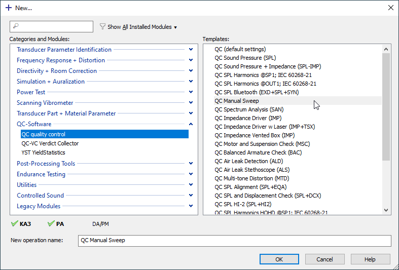
Create a new operation with the QC Manual Sweep operation template for the QC quality control in R&D Framework. For further details see QC manual at chapter QC Software in the KLIPPEL R&D Framework.
KA3 Signal Configuration#
The QC quality control in R&D Framework requires a separate routing within the KA3 Signal Configuration:
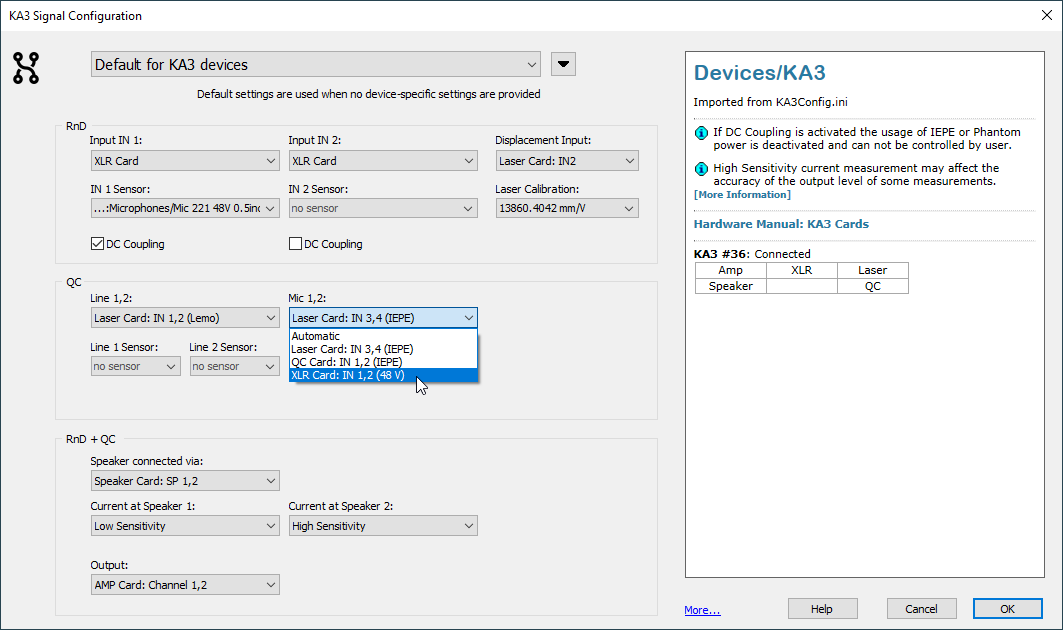
At the QC input routing section the same mic input as used for the RnD input routing should be selected, to be able to use the real time analyzer function of the Manual Sweep operation.
Amplifier Calibration#
The QC quality control in R&D Framework requires an amplifier calibration which could be found at
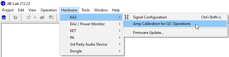
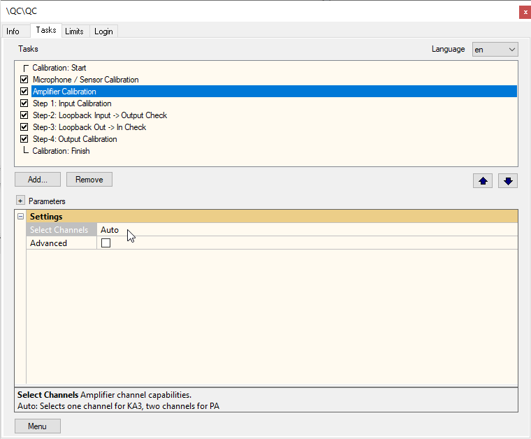
All settings could remain at default conditions.
Just click Calibrate Amp and check its verdict:
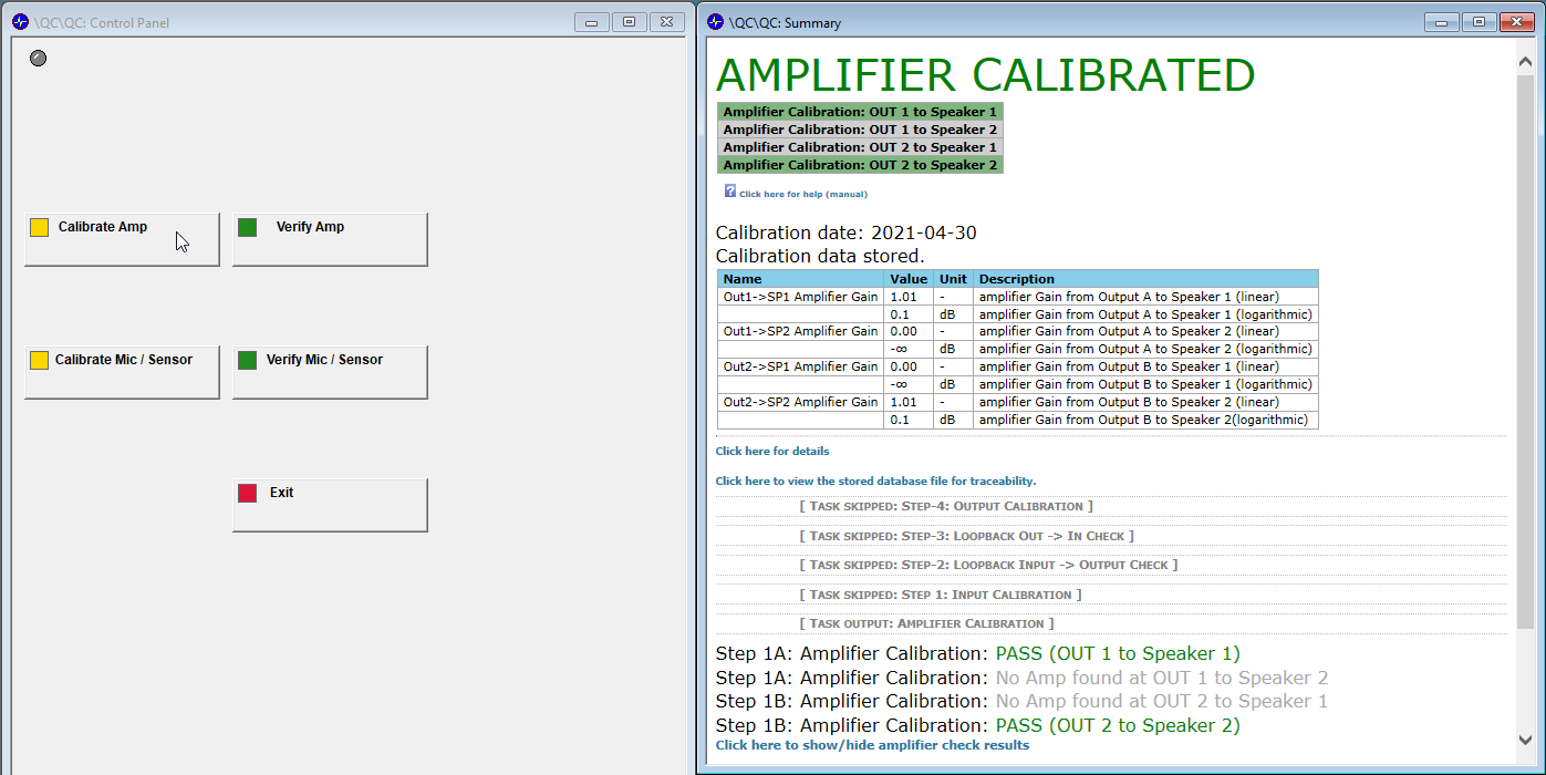
Calibrating the used mic is recommended but not needed if relative results are sufficient.
Exit the Amplifier Calibration
Usage#
Log into the QC Manual Sweep operation:
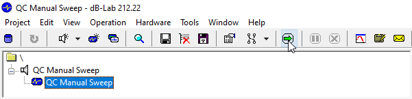
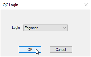
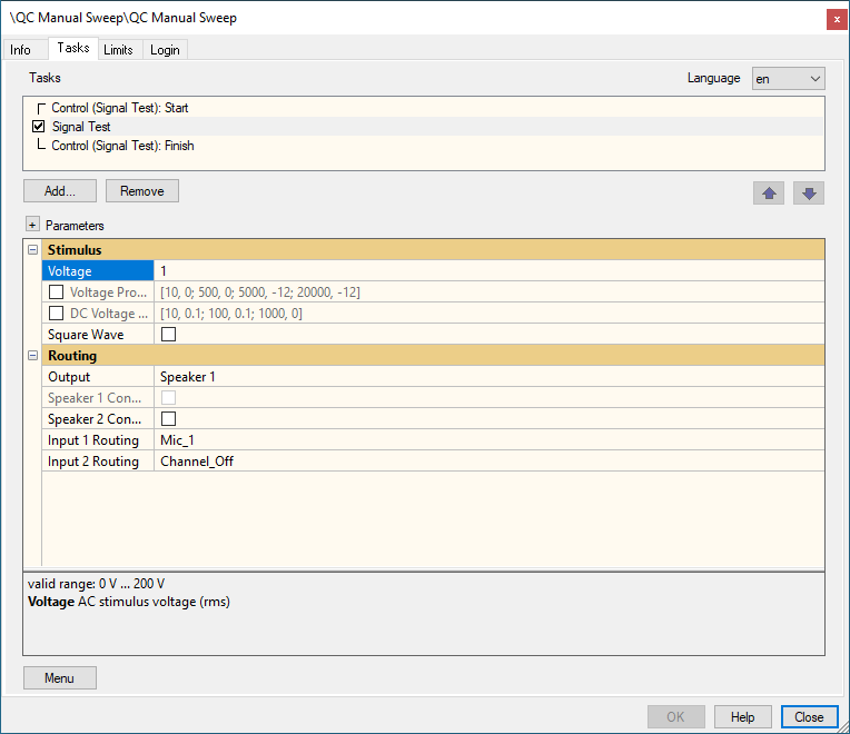
Adjust the starting voltage at the Property Page if the +/- 10 dB from the template value are not sufficient and select the used speaker and mic channel:
Start the Manual Sweep:
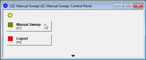
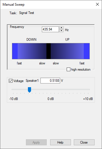
Adjust frequency and voltage for manually checking the DUT at the separate Manual Sweep user interface: