BFS – B-Field Scanner

BFS - Tutorial

Overview

The B-Field-Scanner measures the magnetic flux density B(z,φ) within and outside the magnetic gap of a loudspeaker using a hall sensor probe and robotics changing the position of the probe versus vertical position z and angle φ.

In combination with the geometry of the voice coil the force factor Bl(x) can be calculated, which is an important parameter of the electro-dynamical transducer.

What is the goal of this tutorial?

This tutorial makes you familiar with the B-Field-Scanner.

The tutorial is divided into three parts:

Part 1 will examine existing results of the web example database that comes together with the software.

Part 2 will guide you through your first measurement, which runs almost automatically.

Part 3 gives valuable background information on customizing the measurement according to your needs.

Part 1: Viewing Results

What is the magnetic gap good for?

Within the magnetic gap of electro-dynamical transducers the voice coil is driven by the Lorentz force that is caused by the electrical current trough the voice coil and the magnetic flux density within the magnetic gap.

One of the most important lumped parameters of an electro-dynamical transducer is the force factor Bl(z).

Magnetic flux density B(z)

Example data used in this manual is stored in the Web Example database. If not downloaded already, get it from the latest R&D release <https://www.klippel.de/go/current-rnd-release> and open the web-based database.

See also

View Results for general information on how to download this database, open and view results in dB-Lab.

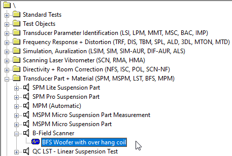
Please navigate to: “Transducer Part + Material (SPM, MSPM, LST, BFS, MPM)B-Field ScannerBFS Woofer with over hang coil” Double-click this operation to display the most important windows.

Web Example Database \\ Transducer Part + Material (folder) \\ B-Field Scanner (object) \\ BFS Woofer with over hang coil (operation)

Magnetic flux density B versus measured height z

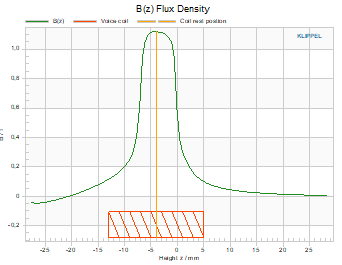
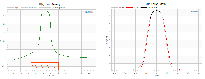
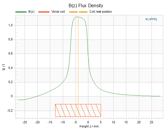
The magnetic flux density B is averaged over the circumference of the magnetic gap and then plotted over the z-axis of the B-Field Scanner.

In this example you could see the outstanding plateau of the magnetic flux density within the magnetic gap of the transducer and the more or less equal decay beneath and above the magnetic gap.

Force factor Bl(x)

Force factor B(x) versus voice coil excursion x

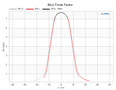
The electrodynamic coupling factor, also called Bl-product or force factor Bl(x), is defined by the integral of the magnetic flux density B over voice coil length l, and it translates current into force.

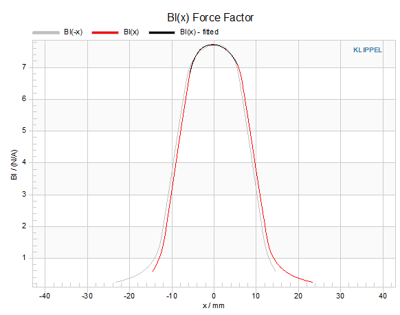
As you can see in the Magnetic flux density B versus measured height z graph the voice coil is set to the center of the plateau of the magnetic flux density. This would be the theoretically best case because it leads to the best symmetry in force factor Bl(x), as you could observe in the Force factor B(x) versus voice coil excursion x graph. The mirrored Bl(x)-curve is an additional feature to check the symmetry of the calculated force factor.

Note

In chapter Modify the calculated results you could learn how to set the position of the voice coil in the measured height z.

Variation Curves

Variation of the magnetic flux density versus angle φ

Variation of the force factor Bl(x, φ) versus angle φ and depending on the voice coil rest position

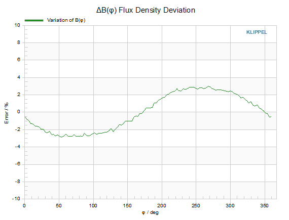
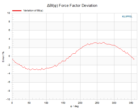
The variation of the magnetic flux density shows the error of the averaged (over height z) flux density relative to the mean value of the flux density over angle φ and height z. Because of the averaging over height z this error obtains for the whole measured height.

The variation of the force factor shows the error of the force factor at the voice coil rest position (φ, x=0) relative to the mean value over angle φ. So, by changing the position of the voice coil on the measured height z you can observe the variation of Bl at this point (plotted versus angle φ).

With these curves asymmetries of the magnetic gap and material defects could be detected very easily. Normally both curves should look similar. If they don’t this could be caused by a very irregular variation of the flux density over height z. It could be observed by changing the position of the voice coil and comparing both error curves at each height z.

More detailed information you could get in the Mean flux density versus z chapter.

Magnetic flux density B(z, φ) contour plot

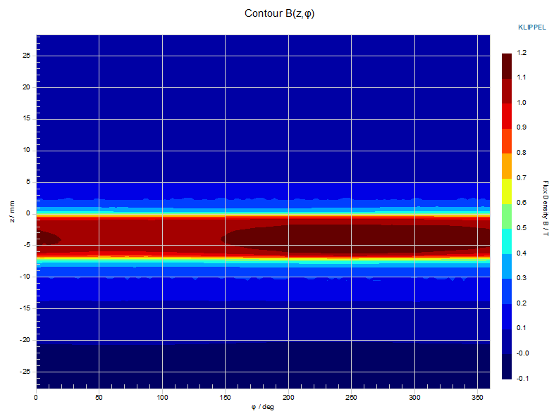
The B-field distribution and variation over the angle can be analyzed within the contour plot of the magnetic flux density over the voice coil gap height \(z\) and angle \(φ\).

Contour plot of the measured magnetic flux density B(z, φ)

Additional results

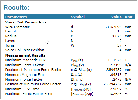
In the Summary window you could see some additional measured results such as the minimum and the maximum value of the magnetic flux density or of the force factor.

There are also shown the voice coil parameters once again for easy monitoring the measurement and for fast comparison with other measurements or different post processing parameter sets.

BFS - Setup (object) \\ Post Processing (operation) \\ Symmary (window)

Part 2: Do your first Measurement

Setting up the Hardware

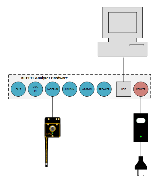
1. Connect the Klippel Analyzer with the power supply delivered by KLIPPEL.

2. Connect the plug of the connection cable to the LASER input of the Klippel Analyzer. Laser Card IN 1 will typically be used for the default laser sensor. Laser Card IN 2 is recommended for the BFS Sensor. Between laser and BFS Sensor the user can select in the dB-Lab / KA3 Signal Configuration menu.

3. Connect the PC and the Klippel Analyzer via USB cable.

Note

For mounting the BFS Sensor to the KLIPPEL SCN hardware please refer to section BFS Sensor mounting.

Starting from Robotics

To become familiar with the B-Field-Scanner you should start the first measurement by using the KLIPPEL Robotics. First you have to click the button New measurement to create a new KLIPPEL database out of a template database. Therefor you have to choose the template database (use the KlTemplate_BFS.kdbx) before you could set the location and name of your measurement database.

By selecting the KLIPPEL provided BFS template the correct hardware setup to use the KLIPPEL SCN hardware for BFS measurements will be loaded. Afterwards the SCN hardware could be calibrated by clicking the button Calibrate Devices. This step goes automatically and you only have to ensure, that the 3 axes of the SCN hardware could move freely upwards and outwards.

For following measurements, the hardware does not have to be recalibrated as long as the calibration LED at the SCN Motor Control indicates a valid hardware calibration. The order during the setup of following measurements could be changed. It is possible to start with the hardware setup according the next DUT and creating the measurement database afterwards. Only for the first measurement above described procedure should be followed.

Note

For the measurement it is necessary to calibrate the BFS Sensor, too. Please refer to section Hardware Setup if your BFS Sensor is not calibrated, yet.

Adjusting the DUT

Now that the database is created you have to adjust your DUT on the KLIPPEL SCN hardware correctly. Therefore, put your DUT in the middle of the rotating turntable of the KLIPPEL SCN hardware as you can see in the Step 1 figure. It is also recommended to mark the orientation of the turntable on the DUT to get reproducible measurement data.

Step 1 - set up the DUT on the scanner turntable

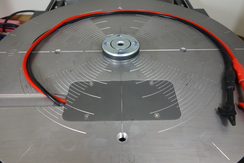
Now move the hall sensor chip directly above the magnetic gap of the DUT but do not dive into it yet. (see Step 2 figure) Set the SCN / Motor Control to manual mode and navigate R- and Z-axis with the Motor Control buttons to the desired position.

Note

It is only possible to measure magnet systems with cylindrical magnetic gaps using the KLIPPEL SCN hardware! For magnetic gaps with other shapes (e.g. rectangular or elliptic) please refer to chapter Measuring special shapes of magnetic gaps in this tutorial.

Step 2 - set up the DUT on the scanner turntable

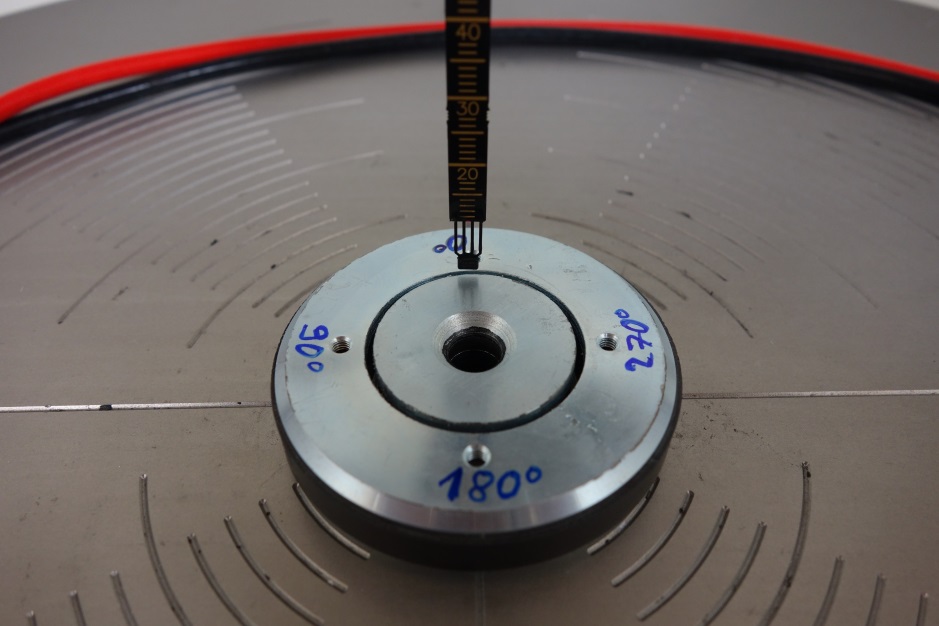
The next step is to turn around the turntable manually with the KLIPPEL Motor Control (MC) for 180° (see Step 3 figure). If the magnet system is not aligned exactly in the center of the turntable you will see that the hall sensor is not exactly above the magnetic gap any more. In this case, please move half of the distance between the hall sensor and the magnetic gap with the KLIPPEL Motor Control (r-axis) and the other half of the way move the magnet system. Now the hall sensor should be exactly above the magnetic gap of the DUT.

Step 3 - set up the DUT on the scanner turntable

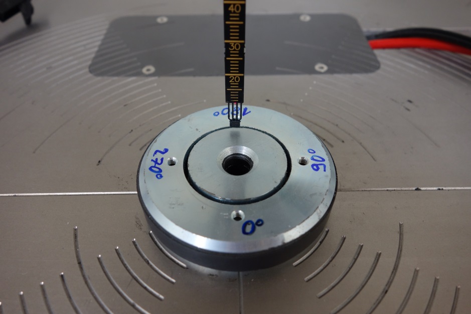
The last step is to move the turntable another 90° around. If the hall sensor is not above the magnetic gap in this step, please move the magnet system so that it is aligned correctly to the sensor. It is very important to move only the magnet system in this step, because the r-axis of the SCN hardware is already set to the correct radius of the magnetic gap!

Step 4 - set up the DUT on the scanner turntable

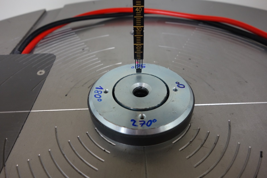
With this last step the DUT alignment is finished. You can now check the alignment by turning the turntable back to 0° and observing the position of the hall sensor above the magnetic gap. The hall sensor should now be exactly above the gap for each angle.

Robotics hardware setup

Now you are almost ready to start your first measurement. But before that you have to click on the button Hardware Setup in the KLIPPEL Robotics to tell the system which hardware to use.

Please first select the Klippel SCN Axes in the shown order (by default the Near Field Scanner axes are selected). If you have done this you could press the button Init all Dimensions to get the current position of all 3 axes. If the KLIPPEL SCN hardware was not calibrated so far, this should be done now.

Robotics Hardware Setup

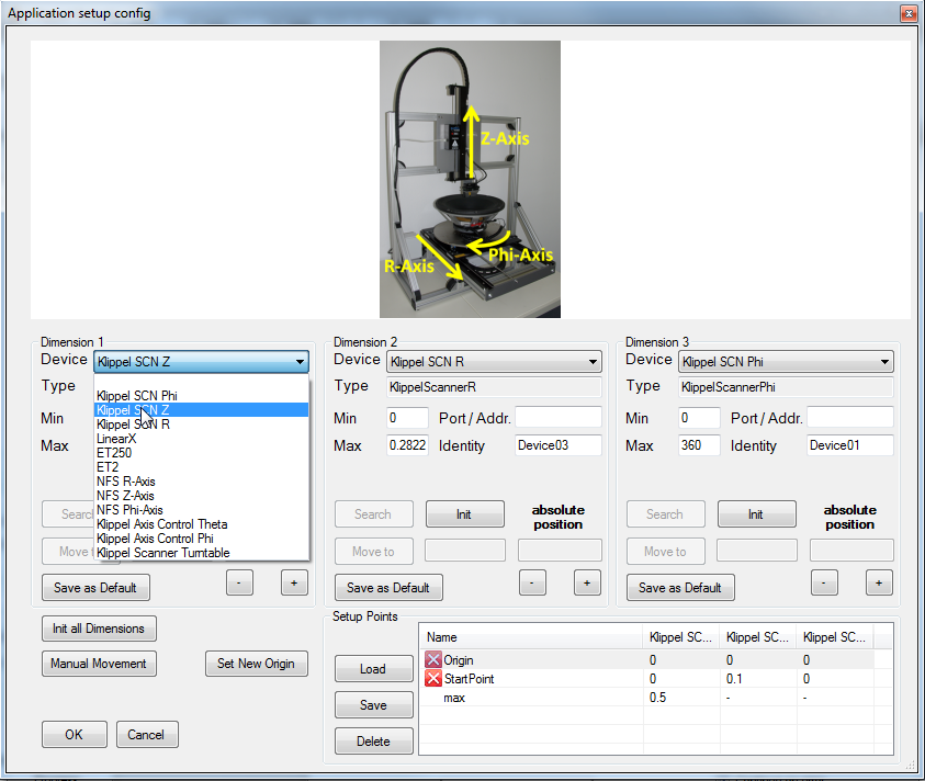
After the calibration and initialization of all hardware axes you have to tell the system at least two points where to start the measurement and where to set the origin of the measurement grid.

Measurement grid Origin

Therefore, move the hall sensor manually to the point that you want to become the Origin of your result curves. It is recommended to use the upper pole plate of the magnet system (see Step 4 figure) because it is an easy to find and repeatable point, but it’s also possible to use any other point as the Origin. If you have moved to the desired point, please click the button Save in the Setup Points section of the Hardware Control to save the current position of the SCN hardware to the Origin point.

Measurement grid Start Point

Now you have to do the same for the StartPoint. This has to be the lowest point of your measured height z. If you are using the upper pole plate as the Origin then it’s good practice to move the hall sensor a certain distance into the magnetic gap either by moving manually with the Motor Control and observing the scale on the BFS Sensor strip or by using the MoveTo mode in the Hardware Control of the Robotics. A nonmagnetic ruler helps to assure that the StartPoint is on a minimum distance above the lower pole plate.

Origin and StartPoint are stored with Z, R and φ coordinates. But circumferential measurements will start independently from the stored φ angle at 0°. Only measurements at a fixed angle will use also the stored StartPoint φ coordinate.

Note

Be careful when using the MoveTo button in the Robotics! If you have calculated the wrong coordinate to move to you might crash your hardware!

When the hall sensor is in the right position for starting the measurement, you could save this point to the StartPoint in the Hardware Control of the Robotics. Now both points should have a green arrow icon next to it and the coordinates are shown for each point (see Confirm setup points before measurement figure).

Finished setup of measurement grid in Robotics Hardware Setup

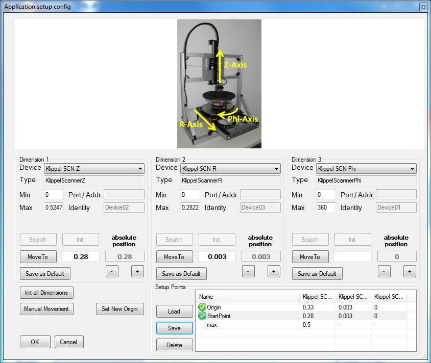
By clicking OK in the Hardware Control window and then Start in the Robotics main menu you will be guided to a last check before the measurement starts. Here you have to confirm that all necessary points are set. If not, you have to go back to the Hardware Setup and save at least the two measurement points mentioned above. Otherwise, you could simply click on Continue and the measurement should start at the starting point that was saved before.

Confirm setup points before measurement

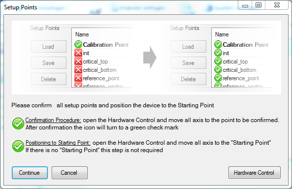
Note

While your measurement is running you could observe the measurement state with the KLIPPEL Robotics. The current step, the total number of steps and the estimated remaining time for measurement is displayed as a progress bar.

When the measurement is finished you could click the button Show Result dB in the Robotics to open the result database. All shown results are already explained in Part 1 of this tutorial.

Part 3: Customizing the measurement

Modify the measurement grid

For automatic measurements with the KLIPPEL SCN hardware the Robotics is a very comfortable tool. In part 2 of this tutorial a measurement with low resolution in height and angle was done. For customizing the measurement grid, go to the KLIPPEL database (e.g. from Robotics with the button Show Result dB) and choose the dB-Lab operation MeasurementArray. With the button Properties you could open the property pages of this operation. On the property page Setup you will find the following input parameters:

Angle Resolution (Phi)

Unit: °

Range: 0 – 360

Defines the step size in the circular movement of the KLIPPEL Scanner hardware

Z Height

Unit: mm

Range: >= 0

Defines the measurement height from the starting point upwards

Z Resolution

Unit: mm

Range: >0

Defines the resolution of the measured height

Higher Precision

Unit: Boolean

Range: [0, 1]

If checked, the middle of Z Height is measured with doubled resolution

With these parameters it is possible to measure almost every cylindrical surface that is in the moving range of the KLIPPEL SCN hardware. The minimal resolution in height and in angle depends on the minimal step size of the SCN hardware that can be found in the BFS Software specification (S47).

If you want to measure only a single layer in circumference, it is possible by setting Z Height to 0. Then only the angle is changed at the height of your initial point in the measurement.

If you want to measure not the circumference but only along the height of your DUT you could set the parameter Angle Resolution to 360°. The measurement will be performed at the angle defined by the StartPoint. This ensures that for each point on the z-axis only a single angle is measured.

With the Boolean Higher Precision you can automatically measure the middle of the measured height is measured with doubled resolution. With this option you could ensure, that the interesting region of the B-Field at the pole plates of the magnetic system is measured with high resolution while the points below and above this interesting region are only measured with half the resolution, just to see the slope of the B-Field.

Modify the calculated results

Out of the measured magnetic flux density the result curves are calculated with the parameters of the PostProcessing script. To change these parameters, you only have to go to the property page Setup of the operation PostProcessing. On this property page you will find the following parameters:

Radius of Coil

Unit: mm

Range: > 0

Defines the mean radius of the voice coil (mean radius = inner radius + ½ coil thickness)

Height of Coil

Unit: mm

Range: > 0

Defines the height of the voice coil

Diameter of Wire

Unit: mm

Range: > 0

Defines the diameter of the voice coil wire with all insulating and air gaps

Note

this value is not used if the parameter Number of Windings is defined, because this is more precise

Number of Windings

Unit: Integer

Range: >= 0

Defines the number of turns at each layer

Note

If the voice coil has more than 1 layer, don’t type in the whole number of turns but the number of turns at only one layer! Otherwise, your Bl(x) curve will show wrong data!

Number of Coil Layers

Unit: Integer

Range: >= 1

Defines the number of layers of the voice coil

Coil Rest Position

Unit: mm

Range: > - Z Height < Z Height

Defines the rest position of the voice coil when mounted into the magnetic gap relative to the origin of BFS measurement (defines the zero position of the Bl(x) curve)

Switch Polarity

Unit: Boolean

Range: [0, 1]

Inverts all measured data for post processing

Note

The PostProcessing could be performed as often as you want if measurement with the KLIPPEL Robotics has finished. You could easily change the parameters of the PostProcessing and recalculate your data. Please do not change any parameter in the MeasurementArray! This won’t delete your already measured data but it causes a lot of trouble if you want to reproduce your measurement!

The parameters that define the geometry of the voice coil have to be set very accurately to get reliable Bl(x) data. Please note that the coil wire diameter is not the preferred one for calculating the coil length. It is recommended to enter a value for the number of windings instead because this leads to a substantially better calculation of the coil length.

It is also very important to enter only the number of turns on a single layer if the voice coil has more than one layer. The absolute number of coil wire turns is calculated automatically from the number of layers and the number of turns at each layer.

The parameter Coil Rest Position represents the distance between the origin that is defined in the Hardware Setup of the KLIPPEL Robotics and the voice coil rest position. So, if you know the exact rest position of the voice coil relative to the point Origin from the Hardware Setup in the Robotics just type in this value here. If you don’t know this distance you could easily search for it by finding the point where the Bl(x) curve and the mirrored one are showing the best symmetry.

If you want to pause your measurement and have a look to the previous measured data, you could easily stop the automatic measurement, go to the database and perform the PostProcessing manually. If you want to resume your measurement just close the database and continue with the KLIPPEL Robotics.

Measurement center point

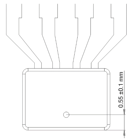
The hall sensors chip center is defined about 0.55mm above its lower edge. Because of this, all measurement results are shown with this offset of 0.55mm to the measurement grid points.

Center position of hall sensor

B-Field orientation

Depending on your DUT and on the direction of the hall sensor in the magnetic gap you may get a negative B(z) curve and also negative Bl(x) values. To compensate for that you could easily invert all measured data by setting the parameter Switch Polarity.

Speeding up the measurement

The properties of the TRF script in dB-Lab are already set for proper working with the BFS and don’t have to be changed in normal case. However, if you want to make the measurement a bit faster, you could reduce the measurement resolution (and thereby the measurement time) in the TRF property page Stimulus.

Note

By doing so, you may get problems with noise if you are measuring low magnetic flux densities. It is also not the measurement time for TRF but the movement time of the SCN hardware that makes the whole measurement slow. So, if you want to really speed up the measurement think of reducing the number of points and not reducing the accuracy at each point!

Measuring special shapes of magnetic gaps

The automatic measurement with the KLIPPEL Robotics and SCN hardware allows a circular moving in cylindrical magnetic motor systems. It is not possible to measure magnetic gaps with rectangular or elliptic shape automatically.

In this special case you could either use the BFS Sensor as hand-held probe (see Reference / Hand-held operation) or perform several measurements at fixed angles. Each of these measurements will only move the BFS Sensor upwards but not circular so that the Sensor won’t be damaged. φ resolution has to be set to 360° (parameter Angle Resolution) and the measurement will be performed at the angle defined by the StartPoint.

With this kind of measurement there is no information in the error charts versus angle φ but you can do it on your own by putting the curves from the different measurements (maybe one measurement each 90° in rectangular magnetic gaps) together in one chart and observe the variation of this set of curves.

Where are the limits

With the BFS it is possible to measure a lot of different magnetic motor systems with different sizes of the magnetic gap and different magnetic fields in them. But what are the mechanical and electrical limits of the BFS?

Mechanical limits

The most critical mechanical limit is the width of the magnetic gap of the magnetic motor system. With the hall sensor that is used for the BFS Sensor it is possible to get into magnetic gaps that are less than 1mm wide. See BFS-Sensor specification (A11) for detailed information about its dimensions and possible magnet gap sizes.

Because of the very long and flexible hall sensor mounting it is possible to measure even in huge automotive speakers, as you can see in the Measuring the magnet system of an automotive speaker figure below.

Measuring the magnet system of an automotive speaker

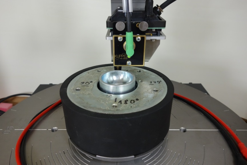
Also, the measurement of magnetic systems that are not completely removed from the speaker is possible (see Measuring a half-dismounted speaker figure below)

Measuring a half-dismounted speaker

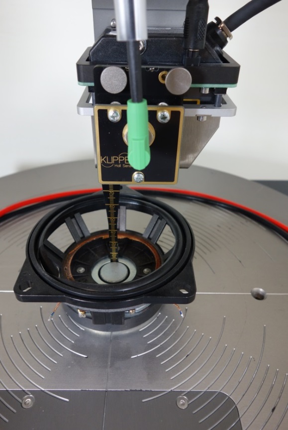
Electrical limits

The electrical limitation is the maximum magnetic flux density of 2.5 T that could be measured. That includes almost all magnet systems that are in use for electro-dynamical transducers. Most magnetic motor systems that have a magnetic gap that is wide enough for the hall sensor have a magnetic flux density < 2.5 T. However, if there should be a wider measurement range, please contact KLIPPEL support to get an offer for a customized version with lower sensitivity, higher maximum flux density measurement range.

BFS - Reference

The force factor Bl(x)

Within the magnetic gap of electro-dynamical transducers the voice coil is driven by the Lorentz force that is caused by the electrical current through the voice coil and the magnetic flux density within the magnetic gap.

One of the most important lumped parameters of an electro-dynamical transducer is the force factor Bl(x)

\[Bl = \overrightarrow {{e_z}} \cdot \int\limits {\overrightarrow B (\overrightarrow {{r_l}} )} \times \overrightarrow {d{r_l}}\]

which is the integral of the magnetic flux density \(\overrightarrow B\) over all points \(\overrightarrow {{r_l}}\) occupied by the voice coil wire with the total length \(l\). The magnitude and direction of the vector \(\overrightarrow B\) at all relevant field points \(\overrightarrow {{r_l}}\) determines the force factor value \(Bl(x=0)\) at the rest position \(z_r\) and the force factor nonlinearity \(Bl(x)\) for any voice coil displacement \(x\).

Measurement process

The magnetic motor systems of almost all electro-dynamical transducers have a circular magnetic gap where the magnetic field of a permanent magnet is concentrated and mostly homogeneous. The DC flux density \(\overrightarrow B (\overrightarrow {{r_l}} ,{i_{coil}} = 0)\) generated by the permanent magnet can be determined either by numerical simulation based on finite element modeling (FEM) or by a direct measurement using a sensor chip.

For direct measurement the sensor chip is placed within the magnetic gap and either the sensor or the magnetic system is moved.

Here the magnetic system is moved in a circular course so that the sensor chip always is placed within the magnetic gap. Additionally the sensor chip can be moved up and down so that the magnetic flux density could be measured step by step both in cylindrical surface and over the height of the magnetic gap. Inserting the sensor chip into the gap also requires free access to the magnetic system and the gap before mounting or after removing the voice coil and diaphragm.

With this movement each point of the magnetic gap can be measured and the results can be shown as a diagram of the magnetic flux density versus height of the magnetic gap and the circumference of the gap.

A mechanical scanner system originally developed for the measurement of cone vibration has been modified for magnetic scanning [1].

Sensor

For direct measurement of the magnetic flux density B a hall sensor is used, which generates a hall voltage

\[{U_H} = {R_H} \cdot \frac{{{I_o} \cdot B}}{b}\]

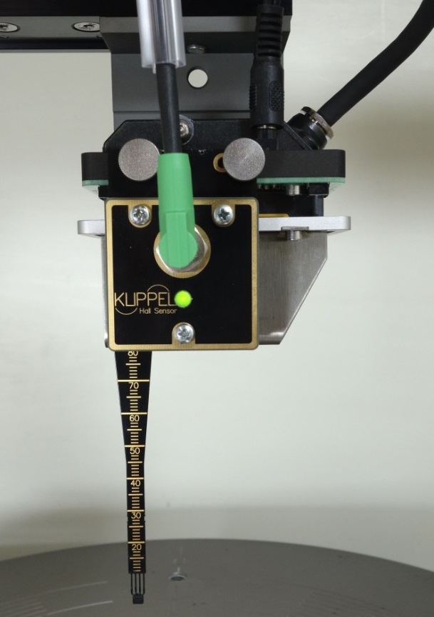
perpendicular to the electric current I₀ in a semiconducting material. For sensitive measurement the probe should be thin (small width b) and a material with a large hall coefficient RH should be used. The small hall element could be mounted on a narrow flexible circuit board simplifying the electrical connection and making the probe particularly suitable for scanning. The width of the gap of most electro-dynamical transducers is relatively small (about 1mm) so the probe has to be very thin and with a small width. For large magnetic gaps (e.g. Subwoofers) the probe also has to be relatively long to reach deep points within the gap, too.

The probe used for the KLIPPEL B-Field Scanner has a thickness of 0.65mm and width of 3.1mm only and can be injected about 80mm deep into the gap while providing a sensitivity of about 1.5V/T which is sufficient for most applications.

B-Field Scanner mounted to the KLIPPEL SCN hardware

Optimized grid

Experiments have been performed to find a scanning grid giving sufficient resolution and keeping the measurement time as short as possible. A sufficient angular resolution requires 4 … 10 points equally distributed over the circumference. About 5 … 10 vertical measurement points are required to measure the rapid decay of the B field at upper and lower side of the pole plate. The vertical resolution may be significantly reduced in the middle part of the gap where the magnetic induction B is almost constant. Measurements at multiple radii are not required because the variations are less than 1 % as confirmed by additional experiments (details see [1]). In total a useful scan of the B field requires at least 100 measurement points.

Postprocessing

With the measured hall voltage and some further information about the voice coil (see User Input Setup) the magnetic flux density

\[B(z,\phi ) = \frac{b}{{{R_H} \cdot I}} \cdot {U_H}(z,\phi ) = K \cdot {U_H}(z,\phi )\]

can be calculated at each measured point of the gap with K as the calibration factor.

The interpretation of the two-dimensional B distribution in the gap can be simplified by calculating further characteristics.

Mean flux density versus z

Assuming axial-symmetry of the magnetic circuit the motor design based on FEM provides a single value for the flux density versus vertical coordinate z. A corresponding value derived from measurement is the mean flux density

\[\begin{split}\begin{array}{c} {{\bar B}^\phi }(z) = \frac{1}{{2\pi }}\int\limits_0^{2\pi } {B(z,\phi )d\phi } \\ {{\bar B}^\phi }({z_i}) = \frac{1}{{{N_\phi }}} \cdot \sum\limits_{k = 1}^{{N_\phi }} {B({z_i},{\phi _k})} \, \end{array}\end{split}\]

calculated by integrating B(z,ϕ) over 2π or by calculating the mean value over all angles equally distributed on the circumference. The Magnetic flux density B versus vertical coordinate z figure below shows the mean value .

Magnetic flux density B versus vertical coordinate z

Force factor versus x

According to the basic Eq. (1) and the Calculation of the force factor figure below,

Variation of the magnetic flux density versus angle φ

\[\begin{split}\begin{array}{c} Bl(x) = m\int\limits_{ - {N_w}\pi }^{{N_w}\pi } {B(x + \frac{\phi }{{2\pi }}D + {z_r},\phi )} \cdot rd\phi \\ \approx m2\pi r\sum\limits_{i = - {N_w}}^{{N_w}} {{{\overline B }^\phi }(x + \frac{{iD}}{2} + {z_r})} \end{array}\end{split}\]

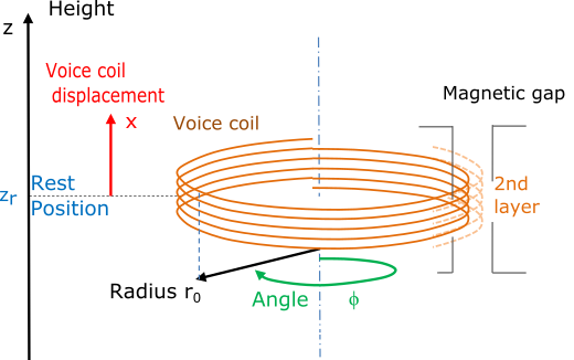
the force factor is a function of the voice coil displacement x from the rest position zr and it is calculated by integrating the flux density B versus wire length l corresponding to an integration over angle ϕ over \(N_w\) windings as illustrated in the Calculation of the force factor figure below.

The parameter m represents the number of layers and D is the diameter of the wire including insulation and winding space.

The Force factor Bl versus voice coil displacement x figure shows the force factor Bl(x) of loudspeaker A taking into account the geometrical data of voice coil. The rest position zr has been determined by minimizing the asymmetry in the resulting Bl(x) curve. The force factor vanishes at high positive and negative displacement but the negative displacement is limited at x=-6mm where the voice coil former hits the back-plate.

Calculation of the force factor by integrating the flux density over the winding length of the voice coil

Force factor Bl versus voice coil displacement x

Flux density variation

The asymmetry of the magnetic field in angular direction is given by the relative variation of the flux density

\[{V_B}(\phi ) = \frac{{{{\bar B}^z}(\phi ) - {{\overline {{{\bar B}^\phi }} }^z}}} {{{{\overline {{{\bar B}^\phi }} }^z}}}100\%\]

with the mean value of the flux density, which is averaged over all vertical scanning points at a particular angle φ

\[{\overline B ^z}(\phi ) = \frac{1}{{{N_z}}}\sum\limits_{k = 1}^{{N_z}} {B({z_k},\phi )}\]

and with the overall mean value which is averaged over all measurement points:

\[{\overline {{{\bar B}^\phi }} ^z} = \frac{1}{{{N_z}}}\sum\limits_{k = 1}^{{N_z}} {{{\bar B}^\phi }({z_k})}\]

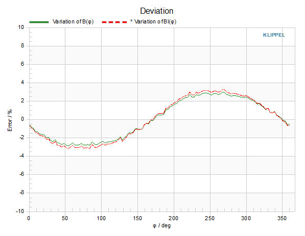
The variation of the flux density of loudspeaker A is shown in the Relative variation of the flux density figure as solid line assessing the asymmetry quantitatively.

Relative variation of the flux density (solid green line) and force factor (dashed red line) versus angle φ of loudspeaker A

Variation of force factor contribution

Whereas the flux density variation considers variation accumulated over the total height \(z_H\) of scanned surface it is more practical to restrict the averaging range to the height of the voice coil and to calculate a new characteristic

\[{V_{Bl}}(x,\phi ) = \frac{{2\pi Bl'(x,\phi ) - Bl(x)}}{{Bl(x)}}100\%\]

which describes the variation of the force factor distribution Bl’(x,ϕ) versus angle ϕ on the circumference of the gap.

The force factor distribution

\[Bl'(x,\phi ) = mr\sum\limits_{i = - {N_w}}^{{N_w}} {B(x + \frac{{iD}}{2} + {z_r},\phi )}\]

is derived from Eq. (5) and the integral over the circumference gives the total force factor

\[Bl(x) = \int\limits_0^{2\pi } {Bl'(x,\phi ) \cdot d\phi }\]

The variation \(V_{Bl}(x,\phi)\) of the force factor density for the loudspeaker A is also depicted in the Relative variation of the flux density figure. With this curve asymmetries of the magnetic gap and material defects could be detected very easily. Normally both curves should look similar.

Requirements

For measurements with the KLIPPEL B-Field Scanner several hardware and software components are required.

Software

Running the scripts requires following software and license from KLIPPEL:

Product	Article	Spec.
dB-Lab (version 210 or higher)	1000-112	F1, S12
Robotics
BFS Software Module	2510-210	S47
TRF Standard Module	1000-900	S7

Hardware

For scanning the B-Field automatically you need the following equipment:

Product	Article	Spec.
Multi-Scanning Workbench, Set	2530-001	C5
LK-H052 Collision Sensor Rev 1.2 (or newer). Older or other Collison Sensors have to be modified.	included in Multi-Scanning Workbench, Set Set 2530-001
Klippel Analyzer 3 Alternative: Distortion Analyzer (Rev 2.0 or newer)	2000-300 (2000-002)	H3 (H1)
BFS Sensor	2510-211	A11
Series 09 replacement Cable Chain	included with BFS Sensor

Hardware Setup

As written above you need the KLIPPEL SCN – Scanning Vibrometer hardware, included in the Multi-Scanning Workbench Set with a suitable laser mounting for performing automatic measurements with the B-Field Scanner.

Scanning System

If there is no SCN hardware set up yet, please read the SCN manual for further information. The Scanning System should be set up completely and be connected to the KLIPPEL Motor Control (MC) before you continue with the setup of the B-Field Scanner.

BFS Sensor mounting

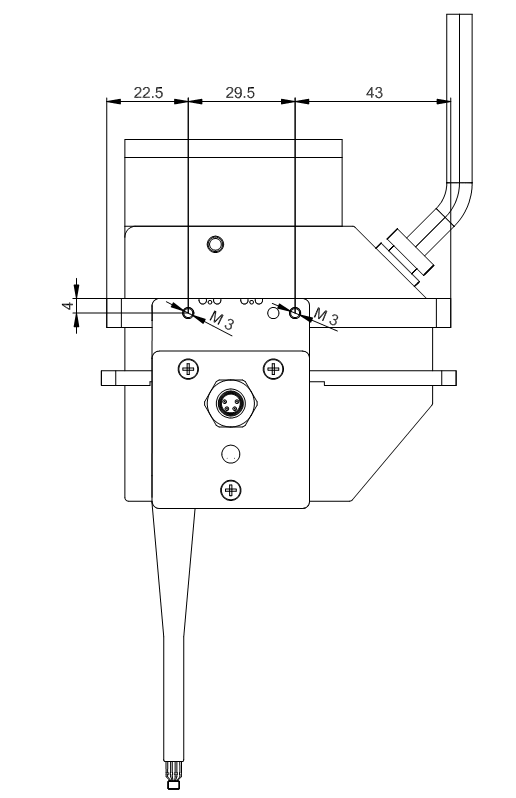
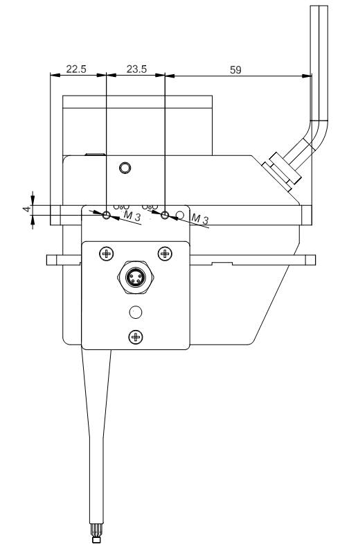
To mount the BFS Sensor to the SCN hardware you need the laser Collision Sensor LK-H052 min. Rev 1.2 with special tapped holes in it (see the Laser mount with tapped holes for BFS mounting figure below).

Laser mount with tapped holes for BFS mounting

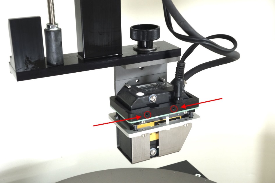
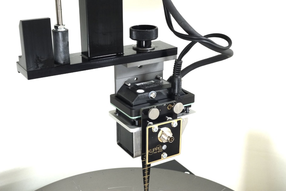
With these holes and the knurled screws you can easily mount the BFS Sensor to the SCN hardware as you can see in the BFS Sensor completely mounted to the SCN hardware figure below.

BFS Sensor completely mounted to the SCN hardware

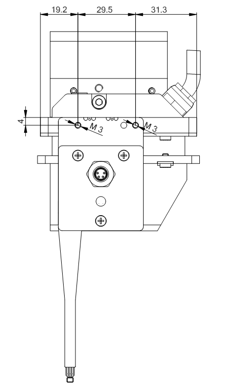
If your SCN hardware has mounted an older revision of the LK-H052 Collision Sensor, LK-G32 or LK-G82 Collision Sensor, follow the instruction to drill just two M3 tapped holes into it.

All measures are in mm:

BFS drill guide for tapped holes at Collision Sensor LK-H052 rev. <1.2

BFS drill guide for tapped holes at Collision Sensor LK-G32

BFS drill guide for tapped holes at Collision Sensor LK-G82

SCN Cable Chain

The original SCN Cable Chain in SCN hardware revision lower than 2.0 gets too tight with the additional BFS Sensor connection cable. The cable chain in these older revisions can easily be exchanged with the included Series 09 SCN Z-Axis Cable Chain.

Calibration

There are two ways for calibrating your B-Field Scanner with a known magnetic flux density:

1. Use a very stable and non-aging reference magnet distributed by KLIPPEL (recommended) (see Reference Magnet)

2. Build up your own reference magnet out of a known magnetic motor system that is measured with a calibrated probe

The calibration process itself is the same for options 1 & 2 above but the following example is done with the recommended reference magnet. For the calibration the BFS Sensor has to be connected to the laser input X of the measurement device (the green lamp at the front of the BFS Sensor should glow). As the procedure differs a bit it is described in separate chapters for KA3 – Klippel Analyzer and DA2 – Distortion Analyzer 2 users.

1. Calibration with KLIPPEL Analyzer

2. Calibration with KLIPPEL Analyzer (legacy method)

3. Calibration with Distortion Analyzer

Reference Magnet

Reference Magnet

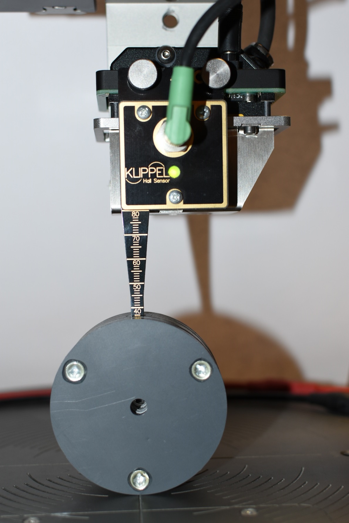
The Klippel distributed reference magnet has the benefit of a very homogeneous magnetic field within a range of +/- 10 mm around its center. So it is very easy to reach the desired magnetic flux density for calibration by diving the BFS Sensor into the reference magnet. These reference magnets are very stable over temperature and resistant against aging effects, too.

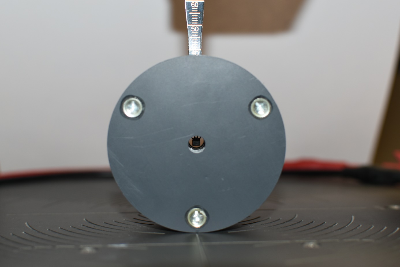
The reference magnet offers a round axial and a rectangular transversal opening for inserting the probe for calibration. For the BFS sensor with its rectangular flat sensor tip the transversal opening as seen in the Reference Magnet figure must be used.

Actual offered reference magnets have an axial through boring which allows to see if the BFS Sensor tip will be in the middle as seen in the BFS Sensor in reference magnet at calibration position figure below. The previous version of the reference magnet without through boring can also be indicated by a slightly smaller outer diameter, 60 mm instead of 70 mm. So the homogeneous magnetic field can be reached with an immersion depth between of 27 mm to 47 mm at the actual reference magnet and 22 mm to 42 mm at the previous reference magnet. The immersion depth could be read directly at the scale of the BFS sensor itself.

BFS Sensor in reference magnet at calibration position

Calibration with KLIPPEL Analyzer

The calibration of the BFS sensor is similar to the calibration of the laser sensor. Please use the BFS Sensor Calibration Object KA3 BFS Sensor Calibration that could be found within the dB-Lab included object templates.

KA3 BFS Sensor Calibration (object) \\ LC LA3 BFS Calibration (operation)

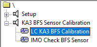
The properties of this operation should already be set for calibration of the B-Field Sensor. Please run the operation in dB-Lab.

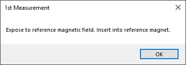
First you should be asked to expose the BFS sensor to the reference magnet field. Use the Motor Control manual mode to move the BFS sensor into the upwards positioned reference magnet or into the refernce field of your own reference magnet. The procedure could also be operated with dismounted BFS sensor.

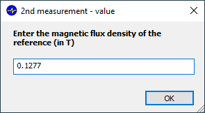
When pressing OK you will be asked to enter the magnetic flux density of the reference magnet you are using. In this example we are using a magnet with flux density of 127.7 mT.

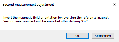
After this you will be asked to invert the magnetic field orientation by reversing the reference magnet. Use the Motor Control manual mode to move the BFS sensor out of the reference magnet, flip it around and insert it again. Or operate it dismounted from the Workbench hardware.

Note

The sign of the final calibration value depends on the direction of the magnetic field you are using for both calibration measurements.

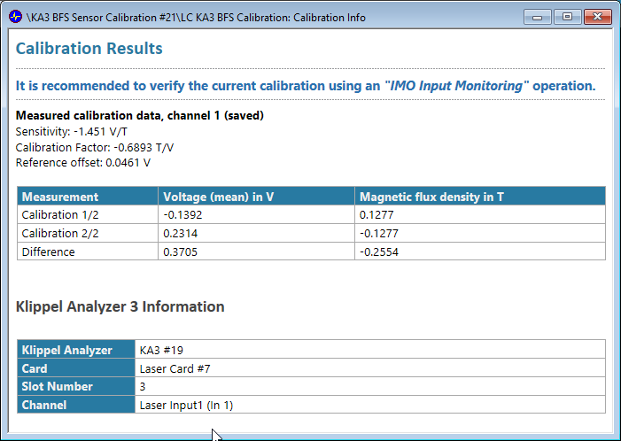
After this is done you will be asked to review the currently calculated calibration value. At this step you still have the possibility to discard the calculated value if you made a mistake during the calibration. For checking the calculated value it will be shown in the result window marked as NOT SAVED.

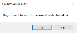
When pressing OK in this message box the calculated calibration value will be saved in the KA3 Signal Configuration and the calibration is successfully finished.

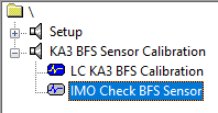
The included IMO – Input Monitoring template should be used to verify the calibration. See Hand-held operation for details.

KA3 BFS Sensor Calibration (object) \\ IMO Check BFS Sensor (operation)

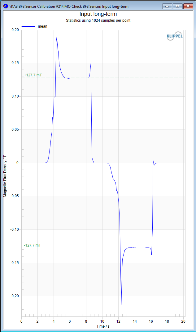
1. Start the operation with the BFS sensor in free-air.

2. Expose the sensor to the positive reference B-field and hold it for a few seconds.

3. Expose the sensor to the negative reference B-field (inverted magnet) and hold it for a few seconds.

4. Stop the measurement and compare the measured values with your reference.

KA3 BFS Sensor Calibration (object) \\ IMO Check BFS Sensor (operation) \\ Input long-term (result window)

Calibration with KLIPPEL Analyzer (legacy method)

The sensor calibration accuracy could be increased with the improved calibration method described above. Although the previous method could still be used and is described below.

• Improved calibration method: 2-step method using doubled reference value for increased accuracy by inverting the reference magnet (changing its polarity). Described above in the chapter Calibration with KLIPPEL Analyzer

• Legacy calibration method: 2-step method using single reference value and free-air reference value. Described below in the chapter Calibration with KLIPPEL Analyzer (legacy method)

Outdated dB-Lab software (<=212.620) without this option should be updated or should obligatory use the legacy calibration method.

Sensor Calibration (object) \\ LC LA3 Hallsensor Calibration (operation)

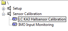
The properties of this operation should already be set for calibration of the B-Field Sensor. Please run the operation in dB-Lab.

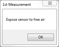
First you should be asked to expose the BFS sensor to free air. Use the Motor Control manual mode to move the BFS sensor up into free air. Move it up to the maximum of the SCN Z-axis or remove the reference magnet from the SCN turn table to have a minimum magnet stray field.

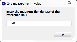
When pressing OK you will be asked to enter the magnetic flux density of the reference magnet you are using. In this example we are using a magnet with flux density of 128 mT.

After this you will be asked to expose the BFS sensor to the magnetic field of your reference magnet. Therefore you can use the SCN system with the BFS mounted to it. Use the Motor Control manual mode to move the BFS sensor into the reference magnet.

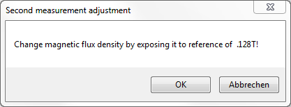
Note

The sign of the final calibration value depends on the direction of the magnetic field you are using for the calibration.

After this is done you will be asked to review the currently calculated calibration value. At this step you still have the possibility to discard the calculated value if you made a mistake during the calibration. For checking the calculated value it will be shown in the result window marked as NOT SAVED.

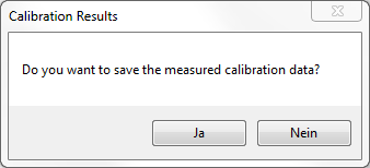
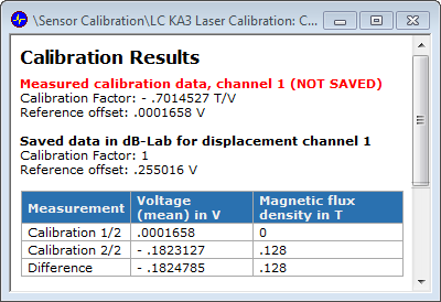
When pressing OK in this message box the calculated calibration value will be saved and the calibration is successfully finished.

The included IMO – Input Monitoring template should be used to verify the calibration. Start the operation and compare the measured environmental B-Field with the B-Field inside the reference magnet. See Hand-held operation for details.

Compensating static offset

Since there is a constant offset in the measurement result which comes from the whole measurement chain, the BFS software has to take this offset into account for measuring correctly calibrated results.

Therefore the last measurement point will be at the upper end of the Z-axis of the SCN hardware under normal operating conditions so that it’s far away from the magnetic field of the DUT.

In case you want to pause the measurement while it’s running you can do this in the KLIPPEL Robotics. When reviewing the measurement results you will see the hint “NOT CALIBRATED” in the Bl(x) and B(z) charts.

It is also possible to run the separate TRF operation that is predefined for the offset compensation manually. It could already be measured during the setup procedure before the automatically controlled measurement procedure gets started. Doing this you can stop the automatically controlled measurement procedure at any point, but still getting referenced results displayed.

Using this legacy method, offset compensated values will be indicated by the reference value which gets displayed in the subtitle of the affected result windows.

Separate TRF operation for measuring the static offset

Calibration with Distortion Analyzer

Note

For calibrating the BFS sensor the firmware version 4.0 or higher is required for the DA!

The Display of your Distortion Analyzer should look like this:

DA default display

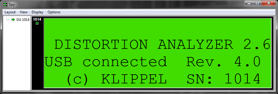
Please press the ENTER button on the Distortion Analyzer to get into the main menu:

DA Main menu (FW version >= 4.0)

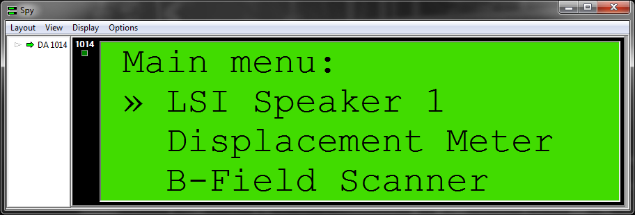
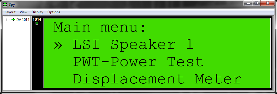
Note

If the main menu of your Distortion Analyzer looks like the following and does not offer the B-Field Scanner submenu, you have to update the firmware version of the DA to ver. 4.0 or higher!

DA Main menu (FW version <= 3.4)

Please select the submenu B-Field Scanner to get to the following display:

DA B-Field Scanner submenu

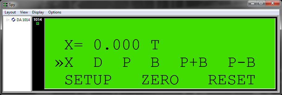
Note

This is the standalone mode for using the BFS Sensor as a hand-held probe for measuring the magnetic flux density directly at every point you want.

For the next calibration step, please select the submenu SETUP

DA B-Field Scanner \\ setup submenu

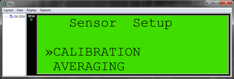
In this menu you can select the Option CALIBRATION to start with the calibration process:

DA B-Field Scanner calibration \\ step 1 - free-air measurement

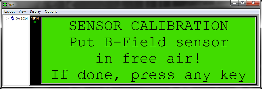
In this first step you have to measure the magnetic flux density in free air with only the environmental magnetic fields (e.g. the terrestrial magnetic field). Therefor remove any magnet system from your SCN hardware and press any key on the Distortion Analyzer

DA B-Field Scanner calibration \\ step 2 - reference field measurement

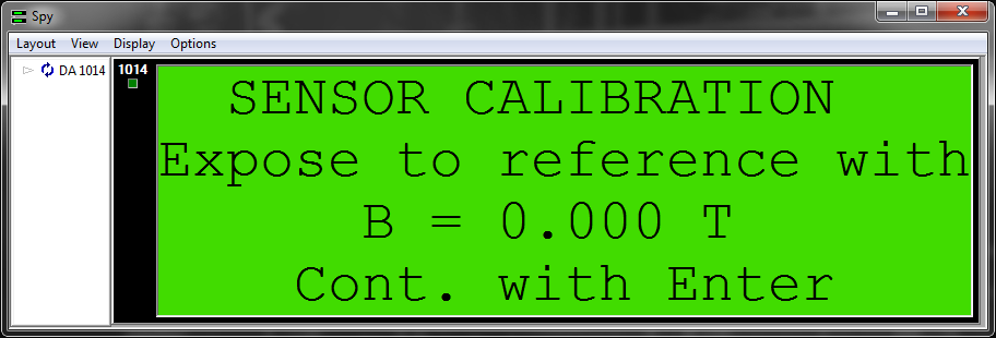
In this step you have to apply a known magnetic field to the BFS Sensor and type in the value of this magnetic field in the DA.

As you can see in the Reference Magnet figure the BFS Sensor could be dived automatically with the KLIPPEL SCN hardware into the magnetic gap of reference magnet to reach the desired magnetic flux density for calibration.

The reference magnet used in this example has a magnetic flux density of about 128 mT in its homogeneous area. By moving the cursor on the display of the Distortion Analyzer you can easily adjust this value:

DA B-Field Scanner calibration \\ step 3 - input reference field strength

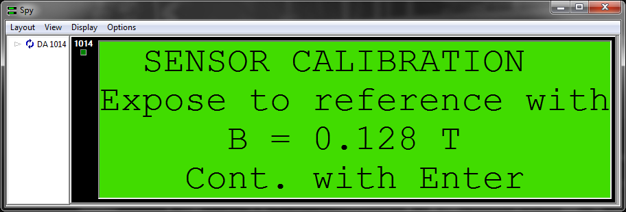
By pressing the button ENTER on the DA the calibration process is finished and you get back to the standalone measurement mode of the DA. Here you can directly check your calibration by reading the measured flux density from the display of the DA:

DA B-Field Scanner calibration \\ step 4 - finished calibration

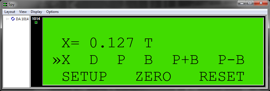
The value could slightly deviate caused by the environmental magnetic field. Depending on the orientation of the reference magnet it could be increased or decreased at the last digit.

Note

For the calibration with the Distortion Analyzer an improved mode is not supported by the device firmware. Although it is possible to use the procedure descibed in Calibration with KLIPPEL Analyzer with following work-around also for the Distortion Analyzer. Use the reference magnet for both calibration steps, flipped around for the 2nd step and input the doubled reference value during the procedure.

User Input Setup

By opening the dB-Lab database you can see 3 operations used for the automatic measurement of the magnetic flux density in magnetic motor systems.

1. MeasurementArray

2. PostProcessing

3. TRF – Transfer Function Measurement

The MeasurementArray is used for setting the grid of the automatic measurement and the PostProcessing includes all information about the voice coil for calculating the force factor Bl(x).

Note

The operation TRF is already set for proper working with the BFS and it is not necessary to touch its properties!

Here is a short summary on the input parameters of the MeasurementArray in the property page Setup:

BFS - Setup" (object) \\ MeasurementArray (operation) \\ Setup (property page)

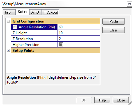
For detailed information about the user input parameters in the MeasurementArray or the PostProcessing please see section Part 3: Customizing the measurement.

Results

The results of the automatic measurement with the BFS consist of the magnetic flux density over vertical axis B(z) and the calculated force factor over coil excursion Bl(x). For each of them an error over the measured angle is calculated.

Magnetic flux density B(z)

Measured static magnetic flux density B(z)

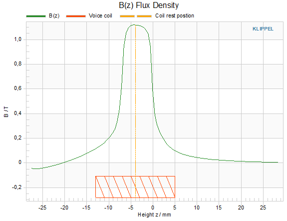
The B-Field is measured directly over vertical axis z and over angle φ of the cylindrical magnetic gap. To show the quantity of this measure in 2-dimensional charts the mean value of the magnetic flux density over the angle φ is plotted versus vertical axis z as you could see in the figure above.

To show the homogeneity of the B-Field in the gap the relative variation of the measured values is plotted versus angle φ as it is shown by the dashed line in the Relative variation of the flux density figure. With this curve you can easily identify asymmetries in the B-Field that can occur when the mounting of the pole plates is not accurate enough or because of systematic errors in magnetizing the magnetic motor system.

Force factor Bl(x)

Calculated force factor Bl(x)

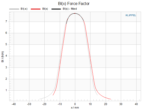
The electrodynamic coupling factor, also called Bl-product or force factor Bl(x), is defined by the integral of the magnetic flux density B over voice coil length l. So for calculation of this force factor the geometry data of the voice coil is needed in addition to the measured magnetic flux density.

With known coil length and height the force factor could be calculated for the measured area in the magnetic field of the gap. To show the force factor versus coil excursion x the distance between the initial point of the measurement and the coil rest position must be known. In the Force factor Bl(x) figure you can see the force factor Bl(x) besides to the mirrored curve (mirrored at coil rest position, gray curve). With the mirrored curve it is possible to identify symmetry problems inside and outside the magnetic gap (for negative or positive coil excursion x).

For the force factor there is also an error versus angle φ to see asymmetries in the driving force of the transducer caused by the magnetic motor system. If there are characteristic rocking modes of the measured speaker this may be caused by an asymmetric magnetic field. Serious errors are above 5% out of the mean value of the force factor [1]. It is also a very characteristic problem when the positive and negative maxima of the error are located in distance of 180° in the error curve. Then you have a typical asymmetry caused by a bad glued motor system.

Note

Because of the static measurement of the magnetic flux density the displayed results for Bl(x) are only theoretically values without any dynamical influence from the current flowing through the voice coil! The feedback effects from the dynamic magnetic field of the voice coil could only be measured with dynamic measurement (e.g. KLIPPEL LSI software). But for small loudspeakers driven by relatively low currents the measurement results between dynamic and static measurement fit very well.

The big advantage of this static measurement is to see all asymmetries of the magnetic system and to see some development issues of the separated magnetic motor system without dynamical feedback effects from the voice coil.

Result variables

BFS - Setup (object) \\ Post Processing (operation) \\ Symmary (window)

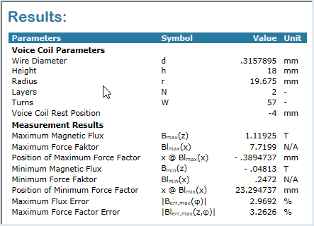
In the Result Variables window some additional values are shown such as the minimum and the maximum value of the magnetic flux density or of the force factor. Also the user input parameters of the voice coil geometry are shown again for a simple and fast monitoring of the measurement and for comparing different measurements.

In this window the software errors and warnings are shown, too.

Supported Modules for Im/Export

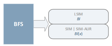
Hand-held operation

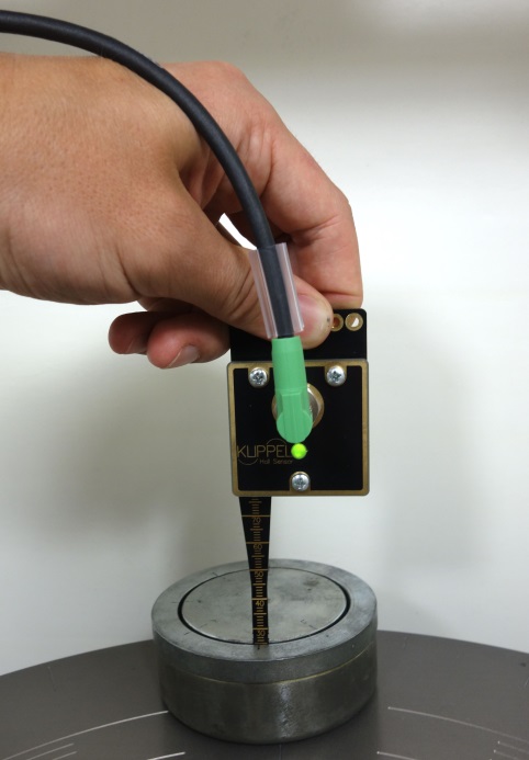
There are some applications where it is useful to have a flexible short term measurement solution with the B-Field Sensor (e.g. if you don’t have the KLIPPEL SCN hardware or you can’t use it for some reason). This could easily be done by using the sensor in hand-held operation.

The measurement values can be investigated in real-time in dB-Lab with KA3 hardware or at the DA2 hardware.

BFS Sensor in hand-held operation

With Klippel Analyzer Hardware

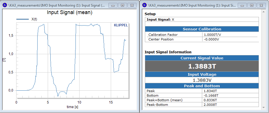
Since the Klippel Analyzer (KA) doesn’t have a display anymore you may use the much more comfortable Input Monitoring (IMO) software within dB-Lab. Simply create a new IMO operation in dB-Lab and select the input X with unit T/V. This way you will get a continuous measurement of the B-Field sensor that is connected to the laser input of the KA. The 2 most important windows for this operation are shown in the Using IMO in db-Lab for hand-held operation figure below. Please refer to the manual of the IMO module for further information.

Using IMO in db-Lab for hand-held operation

With Distortion Analyzer hardware

With the Distortion Analyzer (DA) you can use the Display at the front of the hardware. You have to navigate to the stand-alone B-Field Meter in the menu of the DA (see the Display of Distortion Analyzer as standalone B-Field meter figure).

Display of Distortion Analyzer as standalone B-Field meter

The Distortion Analyzers stand-alone mode B-Field Meter offers following operation modes:

• Absolute values displayed in T (Tesla) measured from the BFS Sensor.

• Relative values displayed in T (Tesla) after an offset has been removed.

• Peak hold

• Bottom hold

• Peak - Bottom (peak to peak)

• Mean value

Malfunction and Troubleshooting

Overview

This chapter will provide information that can help you solve common problems that occur with BFS measurements.

If you cannot find a description here that matches your problem, try these options:

1. Check the dB-Lab Manual that you received with your KLIPPEL R&D System. This document contains the most up-to-date information about known software problems and solutions and installation procedures.

2. Contact us via KLIPPEL support (see chapter How to Report Errors in the dB-Lab Manual)

Software Messages

All error messages in the BFS Software are shown as a message in the Result Variables window. In case of an error also the Log window will be opened automatically to show that something in the code went wrong.

Parameter is missing

Error message:

“Parameter <parameter name> is missing!”

Reason:

The input parameter needed for calculating the results is empty in the property page Setup.

Solution:

Enter a value for this parameter and try running the script again.

Parameter is incorrectly defined

Error message:

“Parameter <parameter name> is incorrectly defined! It must be a <type>!”

Reason:

The input parameter in the property page Setup has the wrong data type for calculation.

Solution:

Change the data type of the parameter to the desired one and try running the script again.

StartingPoint is not defined

Error message:

“StartingPoint is not defined!”

Reason:

The coordinates of the starting point of the measurement are not saved to the Robotics Hardware Setup.

Solution:

Close dB-Lab and go back to the Robotics Hardware Setup. Now move the BFS Sensor with the Motor Control to the point where the measurement should start and save these coordinates as the StartingPoint in the bottom right corner of the window. By doing so the small icon next to this point should change to a green arrow.

Now you could try running the script again.

Hardware Messages

The Robotics will pop up error messages indicating hardware problem with the used SCN Vibrometer hardware and Motor Control.

Hardware Malfunction

Buckled BFS Sensor strip

The automatic measurement with the KLIPPEL Robotics and the SCN hardware is designed to only move upwards and thereby outwards the magnetic gap of the transducer so that the BFS Sensor won’t be damaged.

Anyway, if you are moving the BFS Sensor manually with the Motor Control you could damage it by moving against the DUT or the turntable of the SCN hardware as done in the BFS Sensor strip crashed at the bottom of a magnet figure below.

BFS Sensor strip crashed at the bottom of a magnet

Buckled BFS Sensor strip in free air

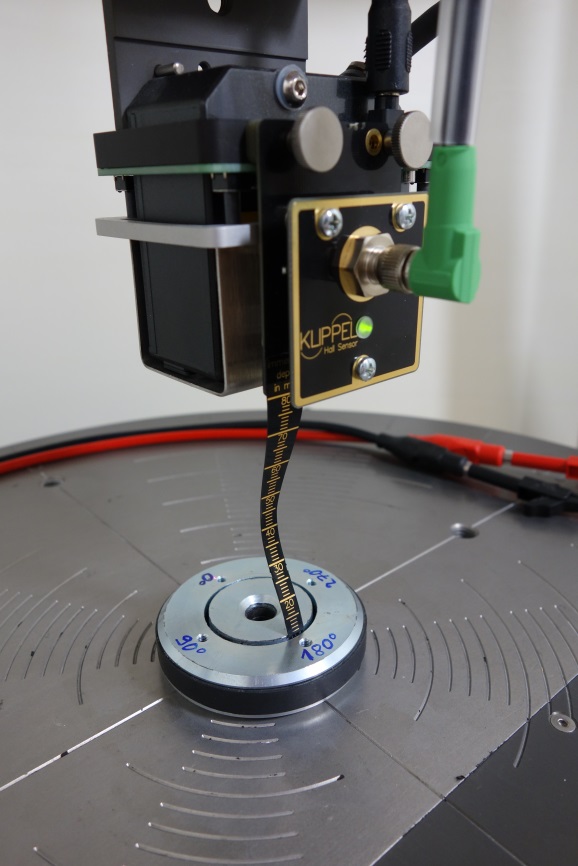
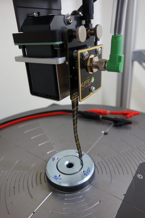
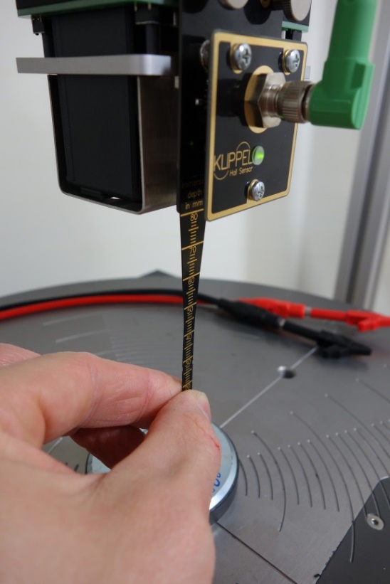
For this reason the BFS Sensor strip is designed as a flexible PCB to buckle first before the small sensor chip at the end of the strip does. In this case please just carefully pull the strip with your fingers as shown in the figure below to straighten it again.

Straighten the strip carefully with your fingers

Maintenance

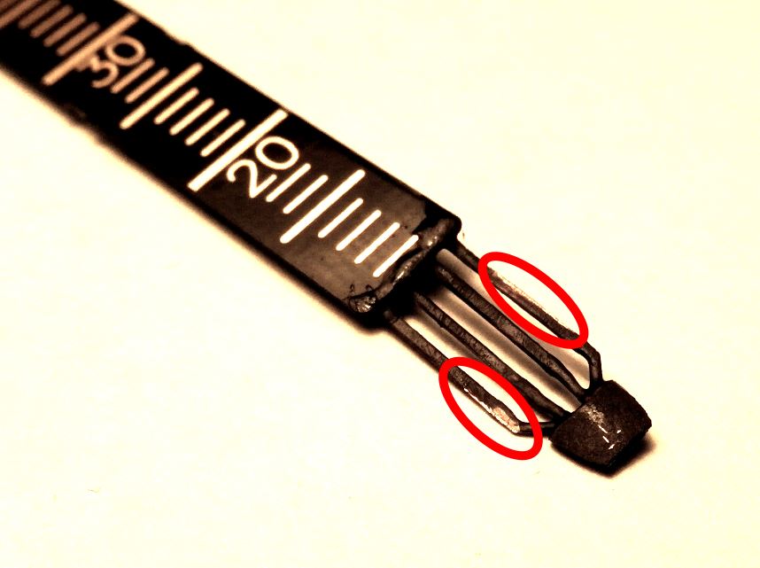
The BFS-Sensor-Chip itself is isolated with a ruggedized black isolation varnish. Under normal operation conditions, the isolation varnish should be withstanding a tremendous number of movements inside magnet gaps without losing its isolating properties. As long as the sensor glides along the walls of the magnetic gap, it will not produce enough friction to abrade the isolation.

If the golden pins get visible, the isolation varnish has to be renewed. The originally used isolation varnish is “Peters SL 1347” (it is very tenable and has good contrast to the golden pins).

A shortcut of any of the pins to a grounded loudspeaker magnet or to any other pin of the senor chip will just cause wrong measurement results. It will not cause defects of the BFS-Sensor itself or the connected Klippel Analyzer.

Abraded isolation at the BFS-Sensor Chip pinss

Literature

[1]

12. Neubert, „Statische Messung des magnetischen Feldes im Magnetfeld von Lautsprechern,“ HTW Dresden, 2010.