Robotics

Overview

The Robotics software is designed for automated execution of all kinds of measurement operations available in the KLIPPEL R&D System. The software is used in combination with rotational and/or linear actuators which move the sensor and device under test automatically to the desired measurement positions.

This allows fast and automated scans of a measurement surface of one-, two and three-dimensional hardware-setups. It is used for various products:

Please find detailed description at:

• BFS – B-Field Scanner

• Near Field Scanner 3D (NFS)

• Polar Far Field Measurement (POL)

• SCN Near Field Add-on (SCN-NF)

Robotics Tutorial

What is the goal of this tutorial?

In this tutorial you are getting familiar with the KLIPPEL Software Robotics. It informs on the required hardware and software. Furthermore, it gives step-by-step instructions how to perform a measurement in combination with the KLIPPEL R&D System.

This will be illustrated based on the example of the Polar Far-Field Measurement (POL) application. This module performs an automated measurement of polar and balloon plots. This will provide a good and understandable guide through the handling of the Robotics.

The Robotics software is covering different kind of automated measurement applications like Near Field Scanner 3D (NFS), SCN Nearfield Add-on (SCN-NF), Polar Far-Field Measurement (POL), B-Field Scanning (BFS). For further information please see the corresponding manuals.

Putting into Operation

This part provides all necessary information on the hardware setup and leads through the installation process of the required software.

Hardware Setup

The following hardware is required:

• KLIPPEL Analyzer (KA3 or DA2)

• 1 to 3 rotational or linear actuators

• Multiplexer (optional)

• Connection cords

• Loudspeaker or another sound source

• Measurement Sensor (Microphone, Laser, Hall-Sensor)

• PC

Note

The kind of required actuators does depend on the measurement setup and purpose.

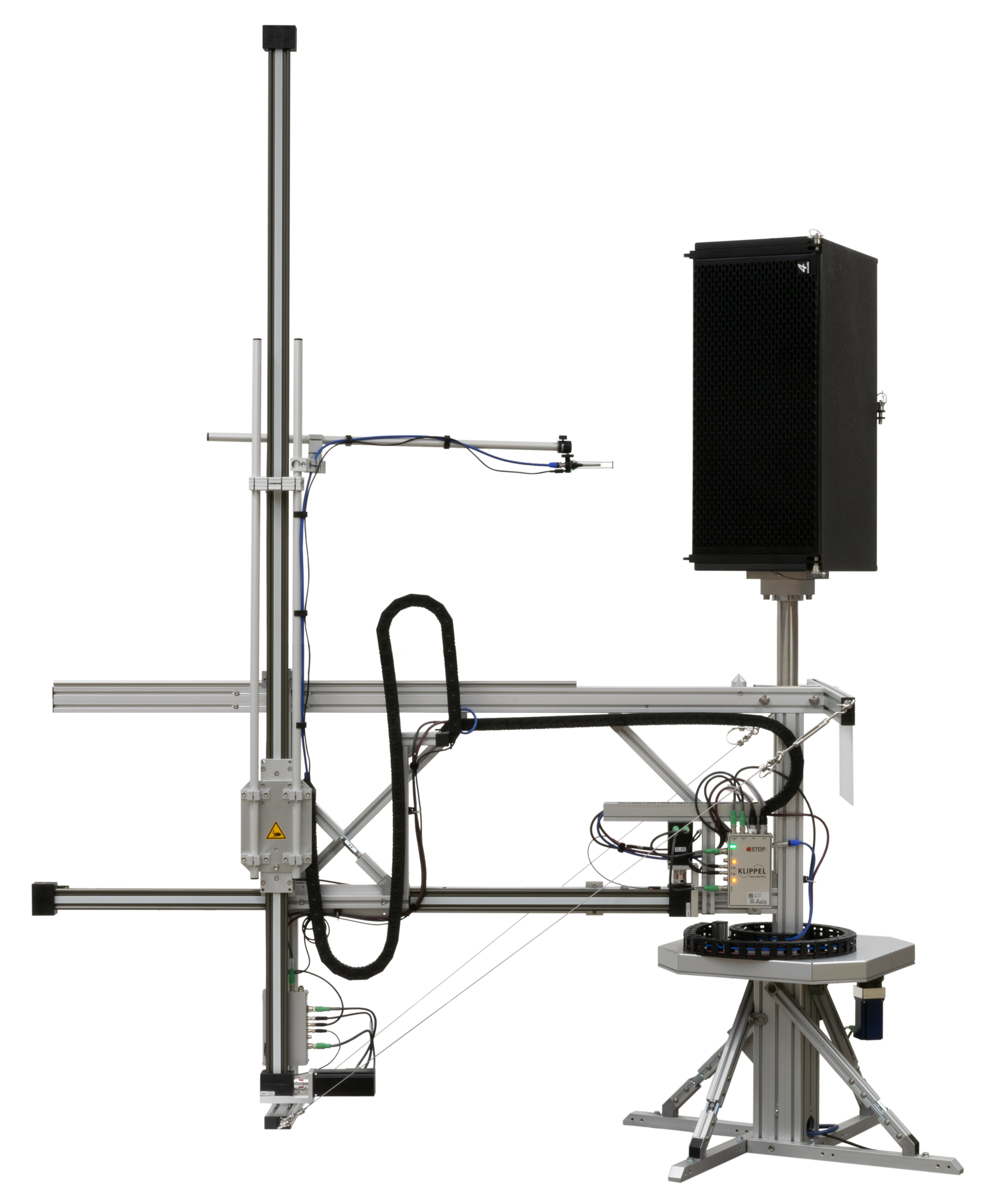
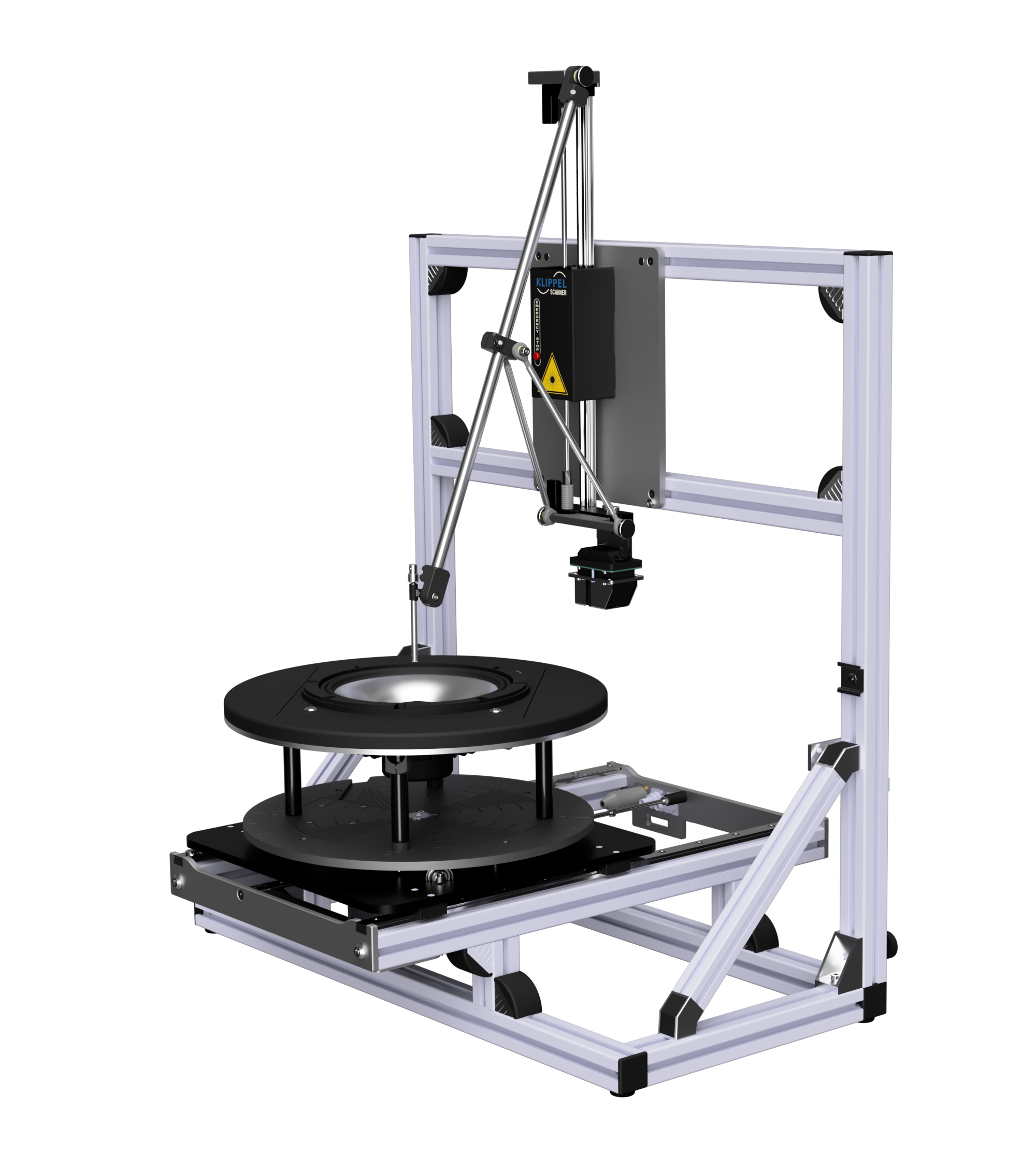
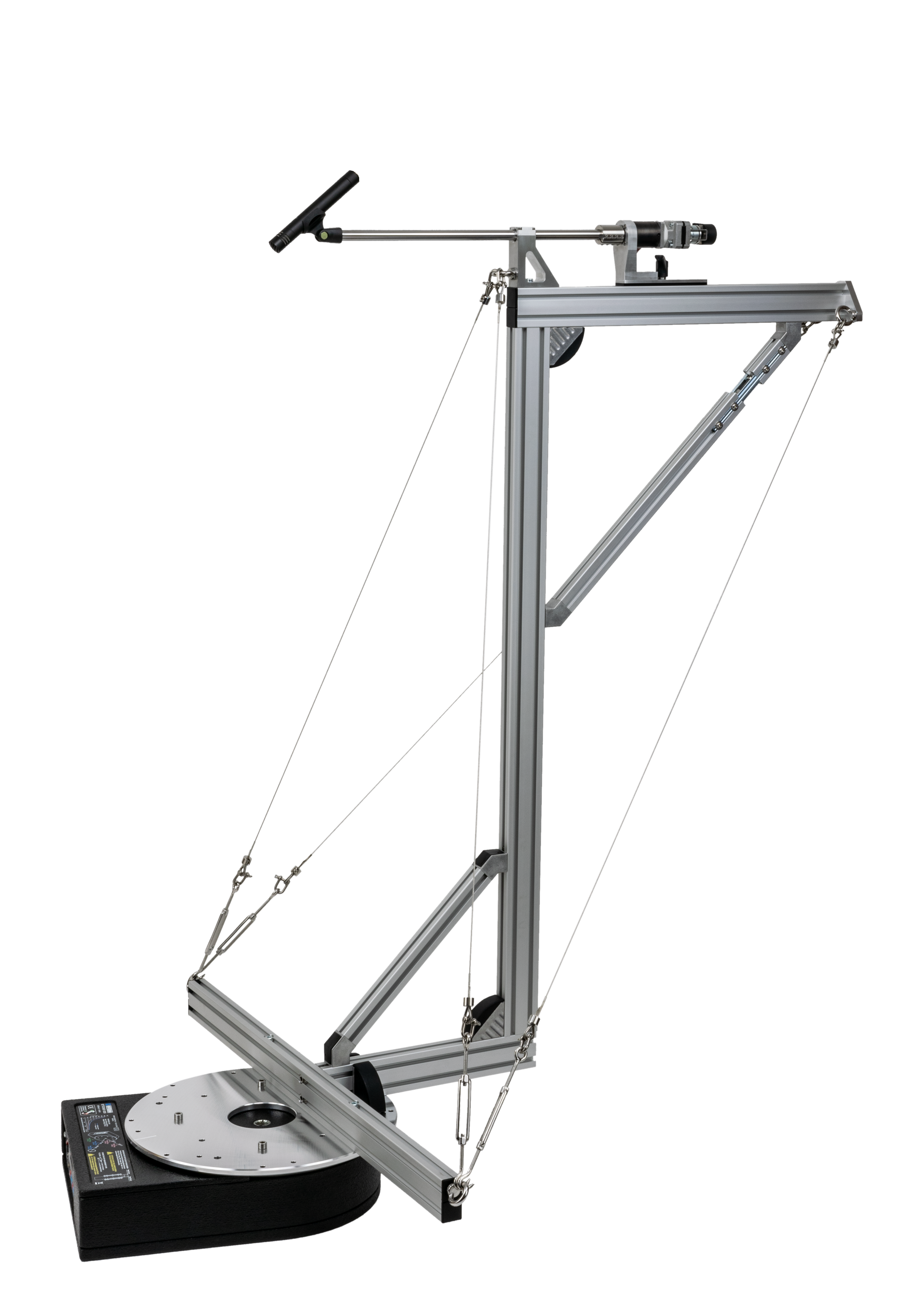
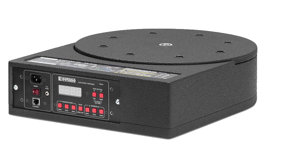
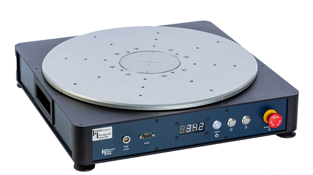
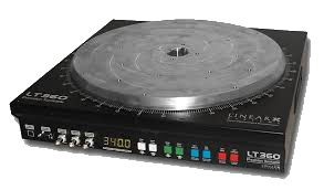
Connect the hardware and connection cords as defined in the manuals for the corresponding measurement operations. Currently, the following actuators are supported by the Robotics:

Klippel Measurement Hardware

3rd Party Measurement Turntables

Software Setup

The following software is required:

• Klippel dB-Lab

• Klippel Robotics

• Licenses of Measurement Scripts (e.g. NFS, POL, BFS)

• Licenses of Measurement Operation (TRF)

Installation Process:

1. Install dB-Lab (see corresponding manual for more information)

2. Install the Robotics software.

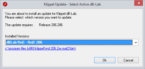
The Robotics software needs to be linked to a version of dB-Lab to work correctly. The installation guide will ask you to choose such a version. Simply select the active dB-Lab version that shall be used with the Robotics and submit the choice.

Choose a dB-Lab version during the installation process

Tutorial 1 – Performing a Measurement

Follow the next few steps to perform your first measurement with the Robotics based on the POL application:

1. Start the Robotics software.

   

2. Select the template database KlTemplate POL.kdbx for the measurement and save your results into a new database by using the button

3. Open the hardware setup by clicking the button .

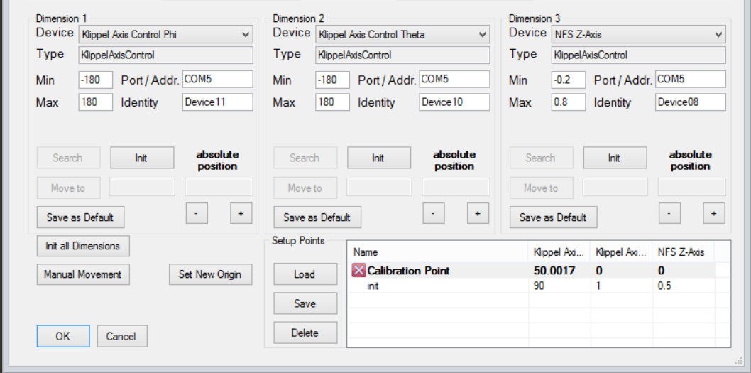
   The following window will open. For other applications than POL the picture might look differently.

   

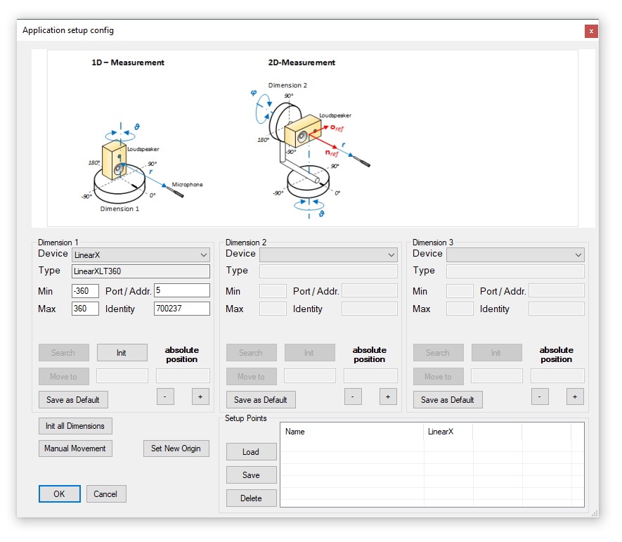
   Hardware Setup in the Robotics for the POL module

Select the connected devices (actuators) for the used dimensions under Device. Simply do not choose a device for a dimension you do not use. After selecting a device and setting the correct Port/Addr (and if necessary Initialize) press Init to check if a connection to this device is possible. Entering a new absolute position in the field next to Move to and press Move to will move the initialized device to the desired position. If an actuator is connected to a wrong port or address you will be informed about that. You may change the corresponding setting in the files devicetypes.ini and config.ini. You can find more information about this issue in the section Configuration of the Hardware Setup. In case you always use the same hardware setup, you only need to do this before the first run. The settings will be saved and loaded automatically the next time you use the Robotics. Submit your configuration when you are done with the setup and go back to the main window. Press Init to initialize the desired devices. Now move them to the wanted origin and press Set New Origin. This will initialize the origin to the current position.

4. Click on to calibrate the chosen actuators.

   In most cases (depends on the moving-hardware), the Calibration-Process will move each device to an outer limit position (synonymous with the most distant point from the center of their axes). Anyway, it is recommended to remove the device under test during the calibration process.

5. Before you start the measurement you may have a look at the settings of your measurement by clicking on the button

   Now, dB-Lab opens the database you defined before to save your measurement results in. Check (and change) anything you need to. Modify the parameters of all operations according to your target measurement performance. Close dB-Lab to continue in the Robotics and to start the measurement.

6. the measurement and wait until it is finished. During the measurement the four diagrams in the Robotics will be updated after each measurement. This way you can have an online-view onto your measurement results.

Congratulations! You just performed your first measurement with the Robotics.

Tutorial 2 – Customizing a Measurement

The second tutorial refers to step 5) of the step-by-step introduction to the Robotics and explains how you can customize a measurement.

Database

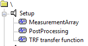
Your KLIPPEL database has to contain the following operations for each object, whereas the first two are part of the POL module:

• MeasurementArray

• PostProcessing

• TRF (or other operation that shall be executed)

Operations in the database

Note

The operations MeasurementArray and PostProcessing must not be named differently in any case.

Configure all the measurement operations the way you want it. For further information take a look into the corresponding manual.

MeasurementArray

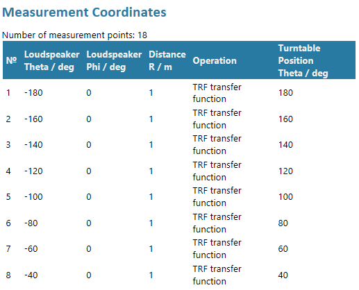
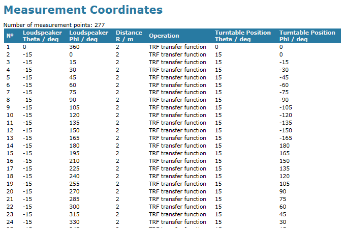
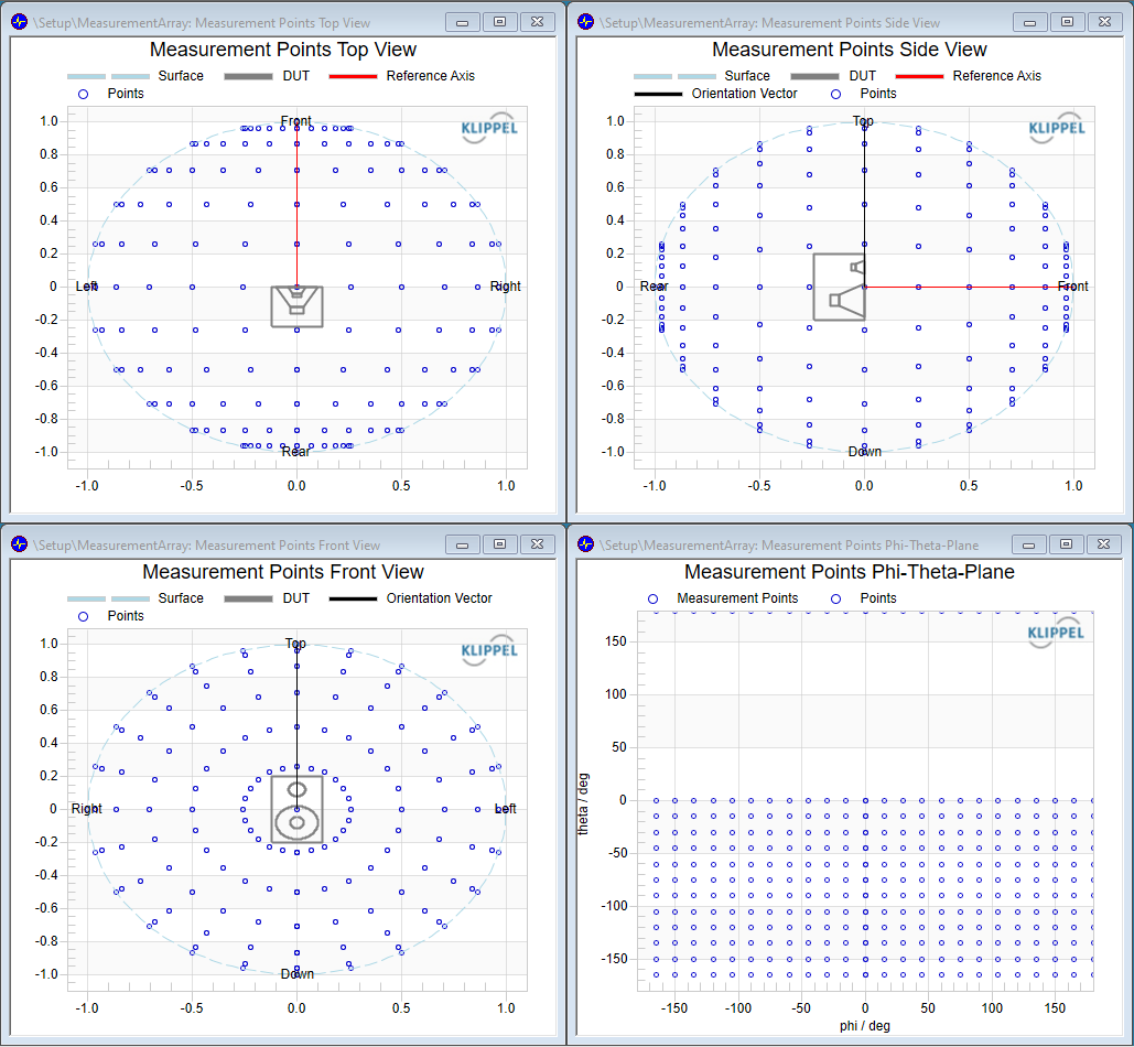
This operation creates your specified measurement grid and saves it into a table for later usage. After running the MeasurementArray –Module this table is shown in the Table Measurement Points window. During the measurement-process, the Robotics will get successively single lines of the generated table. Each line contains the coordinates of the next measurement point and the desired measurement operation. In addition the measurement points are visualized in the other result windows.

You can change the parameters of this operation by opening the Property Page of the operation. In the Setup tab, you can modify all settings regarding the measurement setup and grid. For example, you can adjust the angular resolution.

Property Page of the MeasurementArray operation of the POL module

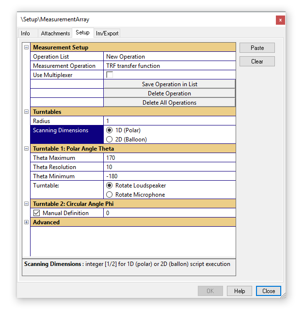
As a result, this operation creates a table containing all the measurement locations as well as the performed measurement tasks.

Table with Measurement Points

More information about the parameters can be found in the Application Note and in the section MeasurementArray in the chapter Robotics User Reference.

PostProcessing

The purpose of this operation in dB-Lab is to post-process your data. The PostProcessing-Operation will be run after each measurement-Operation. So this operation also gives the Robotics the information to move on to the next measurement point when the post processing is done.

The parameters you can specify here in the same way as for the MeasurementArray. Mainly, you can specify if you wish to export your data to VACS and which of the measured data you want to export to VACS. More information on that issue can be found in the chapter Robotics User Reference under PostProcessing.

Robotics User Reference

This reference is of interest for persons who want to use the Robotics as end users and learn more about the basic things that are behind the Robotics.

It explains the measurement concept the Robotics is based on and provides an overview of the graphical user interface. Additional background information on the configuration of the hardware setup are presented.

A parameter reference gives a detailed overview of the different input and output parameters of the operations and describes how to use them correctly. In doing so, this manual provides information in a general sense. Detailed information can be found in the in the Application Notes of the different applications for the Robotics.

Measurement Concept

The Robotics software combines hardware control, to interact with certain actuator, with database automation of the dB-Lab Software.

Interaction of the Robotics with other components

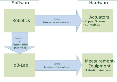
During the measurement the Robotics works as the process master. It controls the actuators to move for example a microphone to a specific measurement position. To perform measurements, do postprocessing or getting information about the next measurement step, the Robotics communicates with the dB-lab database via the automation interface. The measurement it self is controlled by the dB-Lab operation (e.g. TRF) that handles the KLIPPEL Analyzer Hardware (KA3 or DA2).

The operation of the measurement database have the following purposes:

MeasurementArray

Generates the measurement grid and passes on this information to the Robotics

Measurement operation (e.g. TRF)

Execute a measurement e.g. with a logarithmic sweep

PostProcessing

Extract results from the measurement operation and stores the data into the database

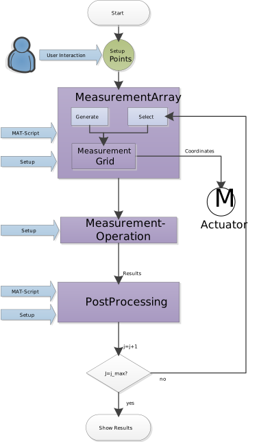
The following figure illustrates the measurement process as a fixed running order. The first step shows an optional user interaction to move the actuators to an initial point. The concept of the initial point is explained in the section Setup Point Concept.

Measurement Process

Graphical User Interface

This section presents detailed information on the graphical user interface of the Robotics.

Graphical User Interface of the Robotics

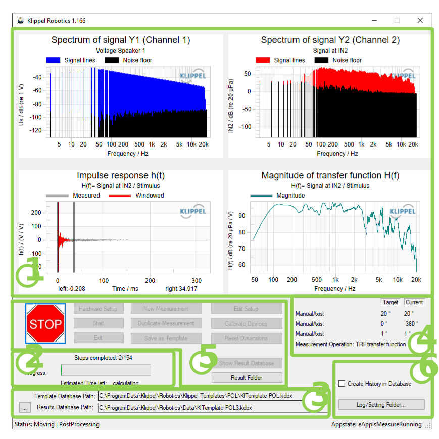
1. During the measurement these four windows will be updated after each measurement. They show selected data, usually seen in dB-Lab.

2. Here you can view the progress of your measurement and how many steps have already been completed. An estimated time for the duration for the rest of the measurement is given as well.

3. This field gives information about the data path of the selected template database and the results path for the result database which contains your measurement results. Thus, this is the place to look up the saving location of the measurement results. With the :kbd:` … ` Button, a Database can be loaded. This is useful to load unfinished databases, or load databases for repeating the post processing of the history

4. Information about the turntable coordinates are given in this area. The shown example is for a one-dimensional measurement setup using the axial axis phi as actuator. Currently, it is on its way from 0° to 10°. The last measurement operation that was performed is TRF1. The result windows (1) still show the results of this measurement at phi=0°.

5. There are different buttons which are mostly available before the start or after the end of a measurement. They fulfill the following functions:

Hardware Setup

Opens a new window, where the user can edit the hardware setup (see section Hardware Setup Window)

Start

Starts a new measurement

Exit

Exits the Robotics application

New measurement

Creates a new measurement from a template the user select in the next step

Duplicate measurement

Duplicates the current database maintaining all results

Save as template

Makes a clean copy (same settings but without results) of the result database

Edit Setup

Opens a dB-Lab instance with the result database to enable a configuration of the measurement settings

Calibrate Devices

Performs a hardware calibration. Dimensions are moved to their reference point starting with dimension 1.

Reset Dimensions

Starts the movement of the actuators to a defined starting position

Show Results

Opens a dB-Lab instance with the result database to view the results of the measurement (available after a successful measurement)

Result Folder

Opens the explorer in the folder, the result database is at.

STOP

Interrupts and stops all movement immediately

6. Additionally, some check boxes are available and fulfill the following purpose

Create History in Database

Creates a copy of each measurement in the result database (otherwise the results of the measurement operation will be overwritten)

Log Settings Folder…

Opens the explorer in the folder, the settings are saved at.

Hardware Setup Window

The Hardware Setup Window provides configurable settings and is used to initialize the hardware for the measurement.

On top, a picture shows the general application of the hardware setup. This picture will change depending on the measurement purpose. It shows which Dimension should be used for which actuator or Device. With the help of the picture, the appropriate Device can be assigned to the desired Dimension. If a Dimension is not used, the blank item in the Device-Drop-Down menu should be selected for that dimension.

The fields Min and Max define the min and max values allowed for this dimension. Adjust carefully, as this is the only safety for not running into any boundary during operation. All values in these fields have to be entered in SI units (meter or degree, respectively).

The fields Port/Addr. and Identity are the main setup parameter of the devices. For example to which port (e.g. COM-port) or network address an actuator is connected and provides a serial number or similar if necessary.

Following settings have to be used for different Turntable devices

Klippel NFS

Identity: unused

Port/Addr: Comport the Device is connected to (e.g. COM5)

ET250-3D

Identity: unused

Port/Addr: Port of host PC which is used to connect to Device / IP Address of the ET250 Turntable (e.g. 6667/192.168.0.20)

LT360

Identity: Identity of the Turntable.

Port/Addr: Comport the device is connected to

After pressing the button Init the corresponding device (actuator) will be initialized (and calibrated if necessary). After that it is possible to move the actuator to a desired position by entering a value in the box below the Init-Button (in SI-units) and pressing the button Move To. The field under absolute position shows the current position of the actuator. Any setup can be saved as default parameters for the selected device by using the Save as default Button.

Hardware Setup Window of the Robotics

Set New Origin

This function defines the current position as new Origin. This procedure is necessary to calibrate the Hardware to any reference point. If the actuators of the NFS are selected, an additional window appears. For details, please read through the NFS Manual.

Manual Movement

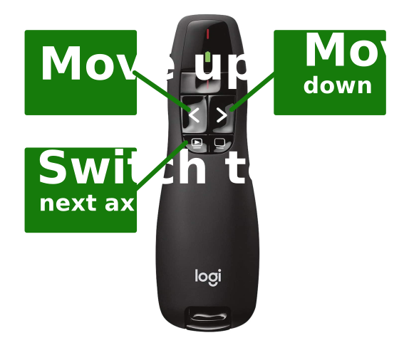
The button : Manual Movement will activate/deactivate the manual movement modus. In this modus, all dimensions can be moved with the remote control or the + / - Buttons. The activated dimension is marked with a yellow marking and may be switched to the next dimension by using the remote control or pressing the . Key. Using the remote control or by pressing the Page Up / Page Down keys, the selected device is moved up or down.

This mode also allows movement, if the devices are ran into the end contacts, or other error conditions apply.

Setup Points

Some Scripts require to enter setup points before the script can be executed. This is done in the Setup points section in the hardware dialog.

There are two different types of setup points:

• Required Points: (marked with a red cross or a green check)

• Not required Points: (no marking)

Required points need to be confirmed before the measurement can be started. This is done by loading the point, and moving all axis to this point one by one. If the point is not where it should be, the hardware needs to be moved to the correct position. By pressing save the current position is saved as the selected setup point.

Configuration of the Hardware Setup

The files config.ini and devicetypes.ini are powerful tools to configure the hardware setup. They allow for a more precise and detailed configuration of the actuators in usage. This section describes how to handle them.

config.ini

This file contains the names of the devices that can be selected in the hardware setup of the Robotics and some more information that are simply read and written by the Robotics, e.g. the data path of the template database. In case of usage of a device that is connected via a COM port to the PC a specification of the COM port is possible here.

[Device01]
Type=KlippelScannerPhi
Name=Klippel SCN Phi
allowedDimension = 3

[Device02]
Type=KlippelScannerZ
Name=Klippel SCN Z
allowedDimension = 1

[Device03]
Type=KlippelScannerR
Name=Klippel SCN R
allowedDimension = 2

[Device04]
Type=LinearXLT360
Name=LinearX
Serial=700237
comPort=5

devicetypes.ini

This file contains device specific parameters as the measurement range (which can also be configured in the hardware setup window of the Robotics) and the number of steps of the actuator.

[KlippelScannerZ]
;general params for device
dev_min=0
dev_max=0.32
dev_res=0.00002
;device specific parameters
z_cal=200
z_min=49335
z_max=65335
stepsPerMmZ=50

Measurement Array – POL

Coordinate System

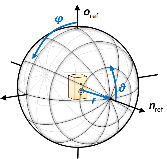
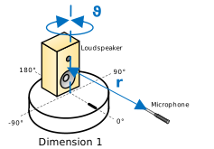
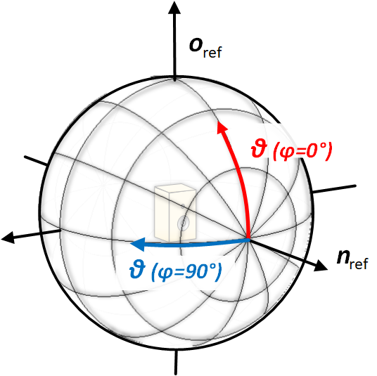
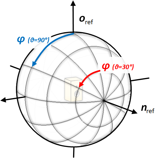
The POL measurement module is based on a spherical coordinates system, that is defined by the radius of the sphere \(r\) and the tw angles, theta \(\vartheta\) (off axis angle) and the phi \(\varphi\) (circular angle).

 The orientation of DUT is specified conform to IEC 60268-21. The reference Axis \(\mathbf{n}_{\text{ref}}\) at \(\vartheta = 0°\) defines the main radiation axis. The orientation vector \(\mathbf{r}_{\text{ref}}\) at \(\varphi = 0°\) defines the orientation of the device under test. It usually points to the top the loudspeaker.

Input Parameters

Measurement Setup

How it Works?

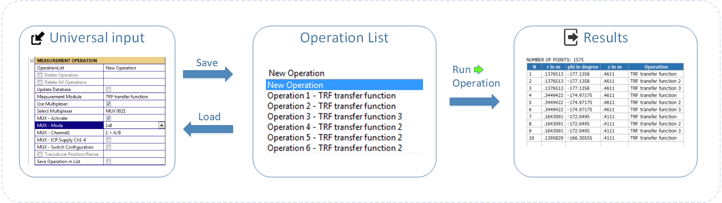
Category Measurement Setup summarizes all parameter for defining the performed measurement. Using the graphical interface multiple measurement operation with different settings can be performed as well as different switching configuration of a multiplexer to measure for example each transducer of a large line array separately in only one scan. Each measurement configuration is stored in the Operation List and will be performed at each point of the measurement grid.

• To edit or show the configuration, select the measurement operation in the Operation List

• To delete one or all operation, click buttons Delete Operation or Delete All Operations

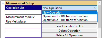
Step 1: Choose Measurement Module

• Select New Operation in the Operation List

• Select the Module for the measurement e.g. TRF transfer function (In case the operation is not available in the List, select “Update List”)

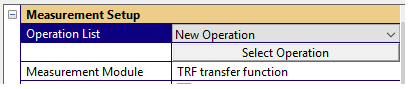
Step 2: Configure Multiplexer Settings (optional)

• To add a switching configuration of a MUX click Use Multiplexer

• Select in the list the MUX that should be switched or update the list to see all available Multiplexer

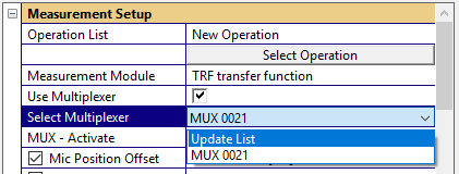
• Click MUX-Activate to activate the selected multiplexer.

• Adjust the switching configuration of the selected MUX e.g. Mode “1x8” 1 to A/B

• Click Switch Configuration to test your configuration and switch all configured multiplexers

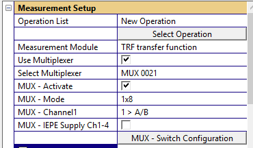
The number of multiplexers is not limited. Just define the switching configuration successively for all devices.

Step 3: Add Position offset (for Microphone Multiplexing)

For using a microphone instead of turntable a position offset each microphone can be added.

To do it insert the offset values for the phi and theta angle in degree. For Example:

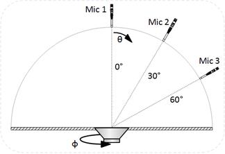
Mic 1 – No Offset

☐ Mic Position Offset

Mic2 – Phi Offset = 0° / Theta offset = 30°

☑ Mic Position Offset [0 30]

Mic3 – Phi Offset = 0° / Theta offset = 60°

☑ Mic Position Offset [0 60]

Step 4: Save Configuration to List

• For measuring multiple transducer separately add a specific Transducer Position/Name (e.g. Driver 1 – Tweeter or Driver 2 – Woofer) During the measurement the data will be stored in separate data containers for the further processing.

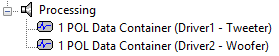
• Clicking Save Operation to List will add the current Configuration to the Operation List

Operation List

List of all operation that will be performed during the scanning process. When selecting an operation of the list, the interface of the properties window is updated and will show the operation settings.

Measurement Module

The parameter defines the measurement operation, which should be performed. [e.g. ‘TRF Transfer Function’]

Use Multiplexer

Activate multiplexer interface

Select Multiplexer

Select a device from the list of all available multiplexers

MUX – Activate

Boolean to active the selected multiplexer:

• ☑ checked: MUX is activated

• ☐ not checked: MUX is deactivated

MUX – Mode

Parameter to select the switching mode of the multiplexer. The following option are available:

• 1x8

  one of the inputs is routed to A and B

• 2x4

  parallel switching of A (Ch. 1-4) and B (Ch. 5-8)

• 4+4

  separate routing of Ch. 1-4 to A and Ch. 5-8 to B

• Custom

  Custom configuration, activate the parameter MUX -Custom Command to send user defined commands to the device

For further information please see: [A8 Multiplexer]

MUX – Channel1

Routing of output A and B for MUX-Mode ”1x8” or

Routing of output A for MUX-Mode ”2x4” and “4+4”

MUX – Channel2

Routing of output B for the MUX-Mode “4+4”

MUX – IEPE Ch. 1-4 (mic. MUX only)

Activates IEPE for Channel 1-4 for a microphone MUX (MUX81-42-BNC - Art.No.:2800-101)

MUX – IEPE Ch. 5-8 (mic. MUX only)

Activates IEPE for Channel 5-8 for a microphone MUX (MUX81-42-BNC - Art.No.:2800-101)

MUX – Custom Command

List of commands for the MUX, for the advanced usage. Using this parameter any possible multiplexer configuration can be switched. See the following example:

'set1x8 5'   //route input 5 using mode 1x8 to output A and B
'seticp 2 1' //activate IEPE supply for Channel 5-8

MUX – Switch Configuration

By clicking the controller, the current MUX configuration will be send to the multiplexer devices. That means the hardware will switch.

Mic Position Offset

Position offset of the microphone to use a microphone array instead of a turntable

Transducer Position/Name

For measuring multiple transducer separately during one scan, a transducer name can be added to save the measurement results in separate data containers.

Save Operation in List

Controller to save current configuration in the Operation List

Delete Operation

Use this controller to delete the selected measurement operation form the Operation List.

Delete All Operation

The controller resets the Operation List

Measurement Hardware

Device under test

Selection of the measurement device. Options:

• Loudspeaker

• Microphone

Radius

Parameter define the measurement distance in meter. The radius r specifies the distance from the center of the turntables (Point of Rotation) to microphone position.

Scanning Dimensions

Parameter to select the Scanning dimension.

• 1D (Polar) measurements with 1 turntable

  

• 2D (Balloon) measurement with 2 turntables.

  

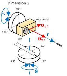
Balloon scan can be also performed with only 1 automatic turntable by using the “Manual Axis”

Select Grid

For 2D Balloon Scans there are predefined grid.

• Custom:

  The Custom setting is generating equidistant spacing for both angles phi and theta. For this grid the minimum, maximum and angular resolution need to be defined

  

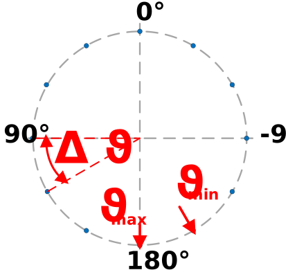
• Polar Vertical/Horizontal:

  Grid is performing a vertical and horizontal polar scan with a defined resolution of theta

  

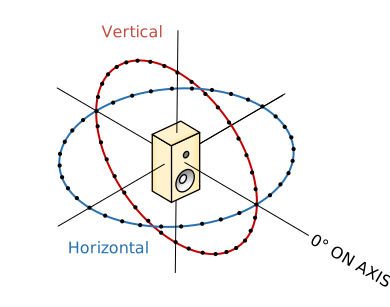
• CEA2034:

  This mode is performing a scan according to CEA2034. (vertical + horizontal polar scan, 10° angular resolution)

  

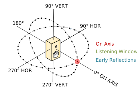
• Full Sphere:

  Performs a full spherical scan. The angular resolution of theta and phi can be specified.

  

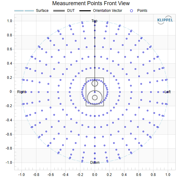
• Half Sphere:

  Performs a scan on a hemi sphere. The angular resolution of theta and phi and the region of the scan (e.g. Down, Down, Down, Down) can be specified.

  

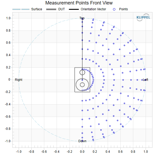
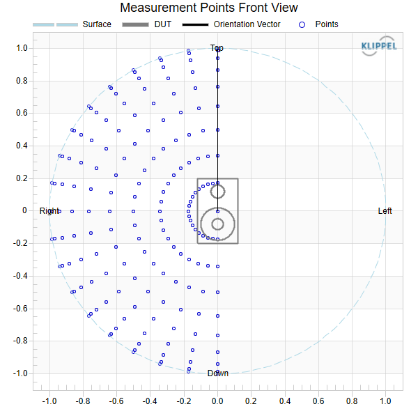
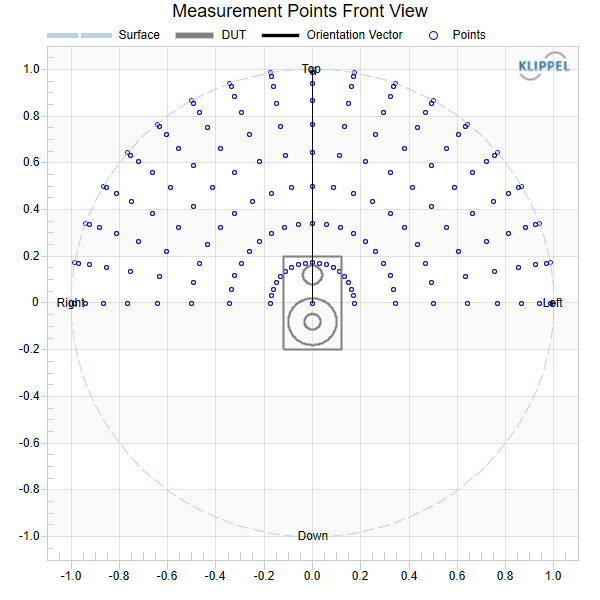
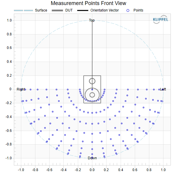
• Quarter Sphere:

  Performs a scan on a quarter sphere. The angular resolution of theta and phi and the region of the scan (e.g. Down-Right, Down-Right, Down-Right, Down-Right) can be specified.

  

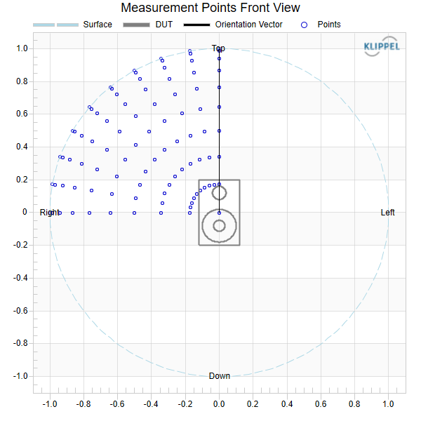
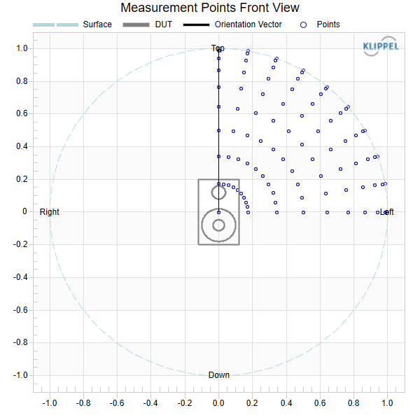
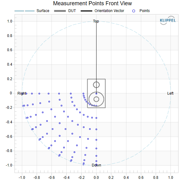
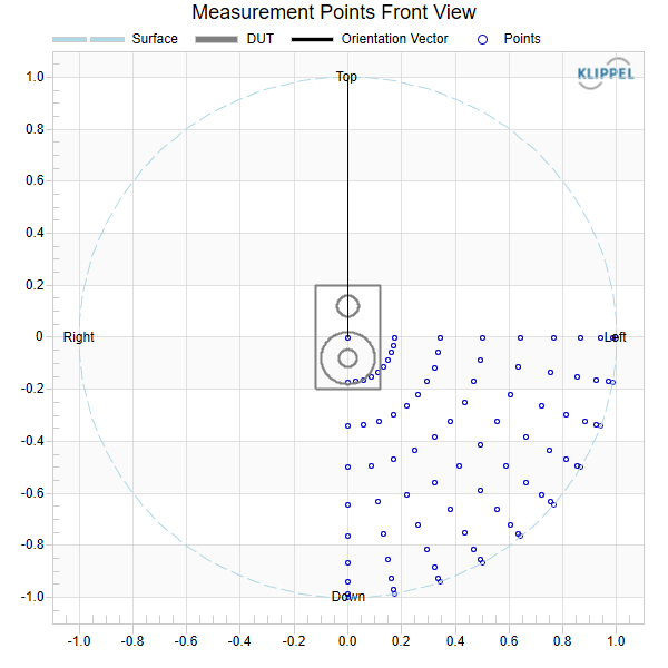
• Table of Coordinates

  Option to define totally freely a driving job a table of coordinates

  Format:

  // column 1:  |  column 2:  | column: 3
  // theta / °  |  phi / °    | r / m
        0              0          1
        5              0          1
       10              0          1
        :              :          :
  

Turntable 1: Polar Angle Theta

The dimension of the 1^st turntable is specified as the polar angle theta. It defines the off axis angle.

Using the following parameters the movement path of turntable can be defined freely.

The point will be linear spaced between the limits.

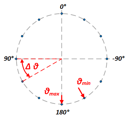
Theta Maximum

\(\vartheta_{\text{max}}\) in \(°\)

Upper Limit of the theta scanning range

Theta Resolution

\(\Delta\vartheta\) in \(°\)

Step size of theta scanning range

Theta Minimum

\(\vartheta_{\text{min}}\) in \(°\)

Lower limit of the theta scanning range

Turntable

Parameter specifies the measurement setup. The turntable can either rotate the loudspeaker or move the microphone.

Note

When rotating the DUT, the turntable coordinates are inverted to assure a measurement in the defined coordinate system.

Turntable 2: Circular Angle Phi

The dimension of the 2^nd turntable is specified as the azimuth angle phi. It defines the circular angle.

Using the following parameters the movement path of turntable can be defined freely.

The point will be linear spaced between the limits.

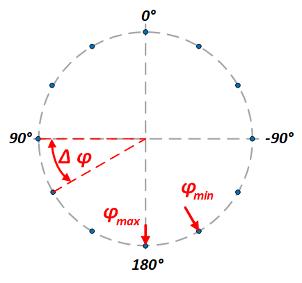
Phi Maximum

\(\varphi_{\text{max}}\) in \(°\)

Upper Limit of the phi scanning range

Phi Resolution

\(\Delta\varphi\) in \(°\)

Step size of phi scanning range

Phi Minimum

\(\varphi_{\text{min}}\) in \(°\)

Lower limit of the phi scanning range

Turntable

Parameter specifies the measurement setup. The turntable can either rotate the loudspeaker or move the microphone.

Manual Definition (for 1D Scan only)

\(\varphi\) in \(°\)

For a one dimensional scan the phi angle can be defined by hand, using this parameter.

Advanced Settings

Sort Measurement Points

To optimize the measurement time, POL supports the following options to sort the grid.

• no Sorting

• Minimum Movement

• Minimum Theta Movement

• Minimum Phi Movement

• By operation

Remove Redundant Point

Using an equidistant angular resolution, the points at the poles are usually measured multiple times (\(\vartheta = 0°\) and \(\vartheta = \pm180°)\). To reduce the number of measurements, these point are measured only once. This reduces the measurement time as well.

• ☐ not checked:      points at the poles are measured multiple times

• ☑ checked:          points at the poles are only measured once

Repeat Measurement

If this parameter is activated the measurement operation will be repeated by the specified number of repetitions

Results

After running, the operation shows the following result windows:

Table Measurement Points

The measurement setup is summarized in the result table which is shown in the picture.

The coordinates and operation for all measurements the column has the following meaning. The Table contains the coordinates, the operation and (for turntable rotation) the coordinates of the turntable.

Measurement Points

These graphs are visualizing the measurement grid in different views (Top, Front and Side) and projected on an unwrapped theta-phi plane.

PostProcessing – POL

Parameter

Setup Parameter - Get

The Parameter Get define the Parameters and Curves, which should be extracted from the measurement operation. They can be freely defined by using the following syntax:

Extraction of Curves:

myCurve = '<Operation Name>#CURVE#<Chart Name >#<Curve Name>'

Extracting of Setup Parameter:

mySetup = '<Operation Name>#SETUP#<Setup Parameter 1>,<Setup Parameter 2>,<Setup Parameter 3>,…'

Extracting of Result Parameter:

mySetup ='<Operation Name># RESULT #<Result Parameter 1>,< Result Parameter 2>,< Result Parameter 3>,…'

Special Commands for TRF Operation:

Extraction of the Measured Impulse Response:

The TRF Impulse Response shows only a downsampled visualization of the Impulse Response, that’s why the curves from this window should not be exported. The “Measured Impulse Response” have to be exported using the following specific command:

myImpulseResponse = 'TRF*#TRF_GetImp';

Note

In case the “Windowed Impulse Response” is required. Please use the extraction with the Im/Export Slide of the Properties Window (see below).

Extraction from the Im/Export Slide

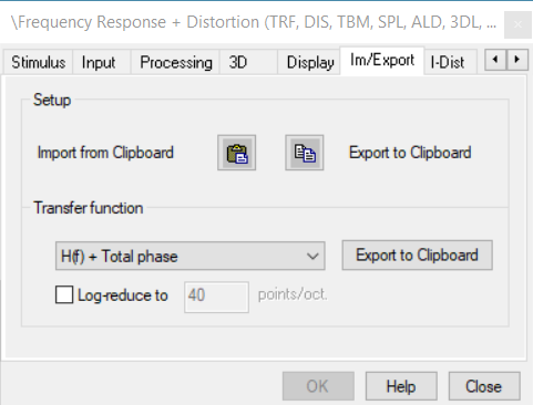
With the following syntax a selected curve from Im/Export slide of the TRF Properties windows can be exported

myTrfExported = 'TRF*#TRF_GetTF';

Example:

The following code shows an example for the Get definition of a measurement with the TRF Module. The PostProcessing operation should extract the Fundamental and curves of the harmonic distortions (2^nd Order, 3^rd Order and THD). In addition the measured Impulse Response and the curve from the Im/export slide should be extracted as well. From the Setup parameters the Stimulus setting are interesting to get the excited frequency range. And from the result the detected Time Delay is extracted.

//Curve Extraction
Fundam = 'TRF*#CURVE#Fundamental + Harmonic Distortion#Fundamental'; //Get Curve “Fundamental” from the Window “Fundamental + Harmonics”
Harmo2 = 'TRF*#CURVE#Harmonic Distortion#2nd Harmonic';                   //Get Curve “2nd Harmonic” from the Window “Harmonic Distortion”
Harmo3 = 'TRF*#CURVE#Harmonic Distortion#3rd Harmonic';             //Get Curve “3rd Harmonic” from the Window “Harmonic Distortion”
THD = 'TRF*#CURVE#Harmonic Distortion#THD';                               //Get Curve “THD” from the Window “Harmonic Distortion”

//Impulse Response and Im/Export Extraction
ImpRes = 'TRF*#TRF_GetImp';     //special command to extract the measured impulse response from a TRF
FreRes = 'TRF*#TRF_GetTF';        //special command to extract the curve from the Im/Export Window from a TRF

//Setup and Result Parameter Extraction
Setup = 'TRF*#SETUP#FMinTRF,FMaxTRF,ResoTRF...';        //Get from the TRF Setup “FMinTRF” + ”FMaxTRF” (Freq. Range stimulus)
Result = 'TRF*#RESULT#TDelayMeasuredTRF';               //Get from the TRF Setup Parameter “TDelayMeasuredTRF” (Measured Time Delay)

Results:

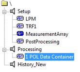
After running the script there will be no results visible immediately. The operation will export the defined Curve to the operation called “POL Data Container”, which is in the Database under the Object “Processing”.

Data Container - POL

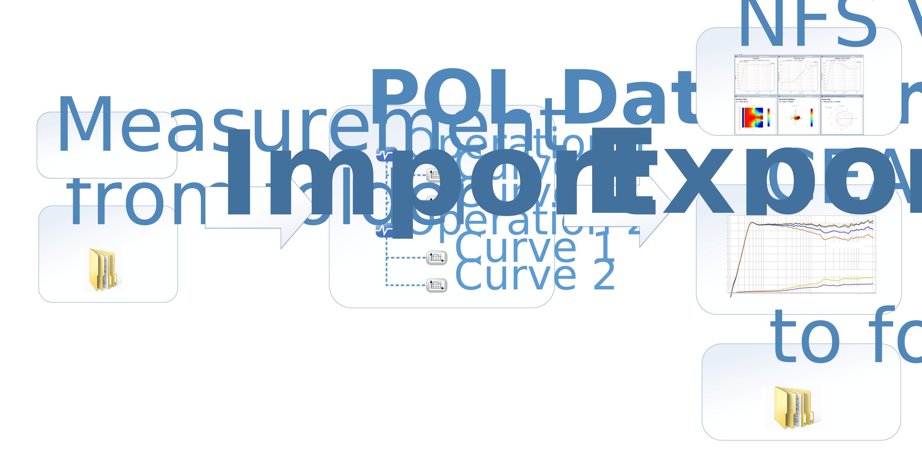
After the measurement is finished all data is stored in the Data Container operation. The data can be transfer into other data formats to analyze the measured data with Visualization Software or external Software like VACS.

Parameter

Data Export

Export Format

Select List to choose the exported format. There are the following choices:

• NFS Visualization: Data can be loaded in the NFS Visualization Software

• VACS ASCII: Data is extracted to a folder on the hard drive in the VACS text format

• CEA2034: Data can be loaded from the CEA2034 operation

Operation

List shows the measured operations. The operation for the export can be selected here.

Curve

Select the curve, which should be exported.

Export Folder

For the VACS export the data is written to a folder. Define the folder path by using this parameter. (for VACS export only)

Round Coordinates – [r, phi, theta]

If the parameter is used the measured coordinates are rounded to the defined accuracy.

Symmetry

For symmetrical devices the measurement time can be reduced by doing only section scans and assume symmetry. To get in the further visualization a full image the symmetry condition can be activated here. There are the following choices:

Half Sphere

• Left ⬄ Right - Horizonal Symmetry

• Top ⇳ Down - Vertical Symmetry

Quarter Sphere

• Right - Top (\(0° \le \varphi \le 90°\))

• Right - Down (\(90° \le \varphi \le 180°\))

• Left - Down (\(180° \le \varphi \le 270°\))

• Left - Top (\(270° \le \varphi \le 360°\))

Rotational

• no phi dependency

Data Import

Import Format

Select List to choose the exported format. There are the following choices:

• VACS: Data is loaded from a folder

• History: Data is loaded from the TRF operations of the History Object in the kdbx-database.

VACS Import

• Source Folder Folder Path, from the data should be imported.

• Interchange Phi and Theta In case a polar scan with the old POL module was performed with the phi axis. The angles phi and theta have to be interchanged. This can be done by activating this checkbox.

History Import

• Import Node Internal database path to the folder or object that contain the data to import.

• Use Settings from Operation The TRF is providing a lot of post processing options e.g. Smoothing or Windows. And sometimes once a POL scan is done it useful to modify some of these settings. By selecting an operation for the setting all parameter can be configured in the Property Page of this TRF and will be applied automatically to the other operations during the import.

• Coordinate Definition When importing data from a History the coordinates must be connected to measurement operations. This is done by a naming convention.

TRF…[<coordinate 1> | <coordinate 2> | <coordinate 3>]

• The parameters R Definition, Phi Definition and Theta Definition are used to extract the coordinate information from the Operation name, from the Object name or set it to a fixed value.

• Data Section to select the data which should be extracted from the Operation of the history. How it work?

1. Select Chart and Curves

2. Add Curves to the List

3. All Curves that are in the Import List will be extracted

Import Name

Data that for storage in the Data Container

Start Import

Button triggers the import

Results

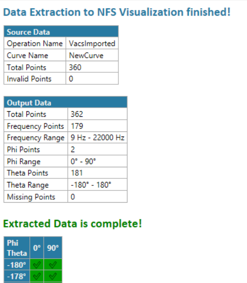
Summary Window

After running the script the Summary window will show information, if the data Im/Export was successful and if the data is complete.

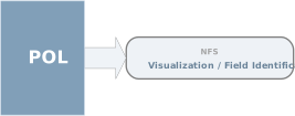
Supported Modules for Im/Export

CEA2034 – POL

The CEA 2034 standard specifies meaningful loudspeaker responses at specific points, for home applications. This is helpful when considering the interaction with a room and when comparing loudspeakers regarding their performance at defined listening positions.

Measurement Data

The CEA2034 requires two polar scan horizontal and vertical with an angular resolution of 10 degree. The measurement distance is specified as

Parameter

Input Operation

The Parameter define from which operation the data is loaded.

Half Space Measurement

For measuring a transducer mounted in a baffle, the CEA Curves are calculated using only the points of the front half sphere.

Reference Input Voltage

All Frequency responses are referenced to that voltage. If deactivated the reference voltage is 1V.

Curve Calculation

As defined in the CEA2034 standard the results curves \(H_{\text{Res}}(f)\) are calculated by a power average of the specified magnitude responses \(H_i(f)\).

\[H_{\text{Res}}(f) = \sqrt{\frac{1 }{n}\cdot\sum_{i=1}^{n}{}\left| H_i(f) \right|^{2}}\]

As specified by the standard, the calculation of the Sound Power and the Estimated In-Room Response includes additional weighting factors \(w_i\). These curvesare calculated by a weighted power average.

\[H_{\text{Res}}(f) = \sqrt{\frac{1 }{\sum_{i=1}^{n}{w_i}}\cdot \sum_{i=1}^{n}{\left| H_i(f) \right|^{2}}\cdot w_i}\]

Result Curves

All curves are referenced to an input voltage of 2.83 V rms at a distance of 1 m

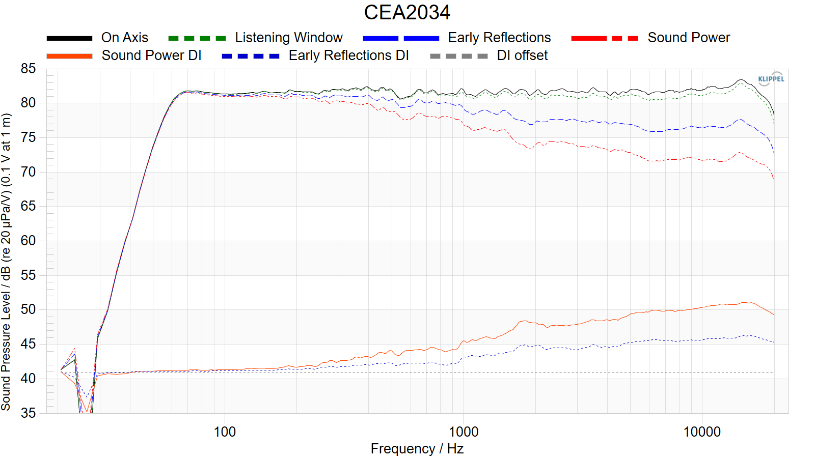
CEA 2034 Summary Window

The summary window defines the standard reporting format of the loudspeaker. It includes the following curves:

On Axis

On Axis SPL Response (at \(\vartheta=0°\))

Listening Window

The listening window curve is a spatial average of the nine magnitude responses in the ±10º vertical and ±30º horizontal angular range.

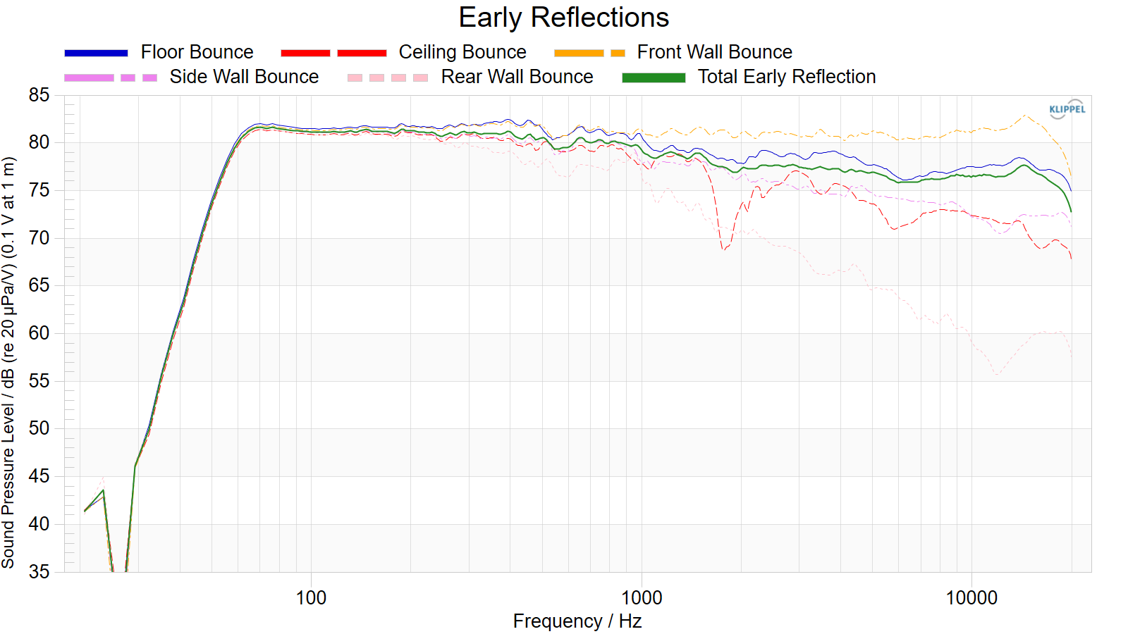
Early Reflections

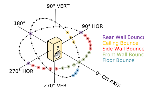
The early reflections curve is an estimate of all single-bounce, first-reflections, in a typical listening room. The definition of the point is shown below.

Sound Power

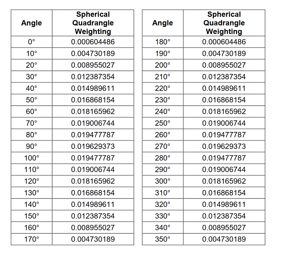
The sound power is the weighted rms average of all 70 measurements, with individual measurements weighted according to the portion of the spherical surface that they represent. The weighting values are shown below in the appendix. Using Eq. (2) the weighted power average is calculated.

Note

For half space measurement mode the weights a multiplied by factor 2.

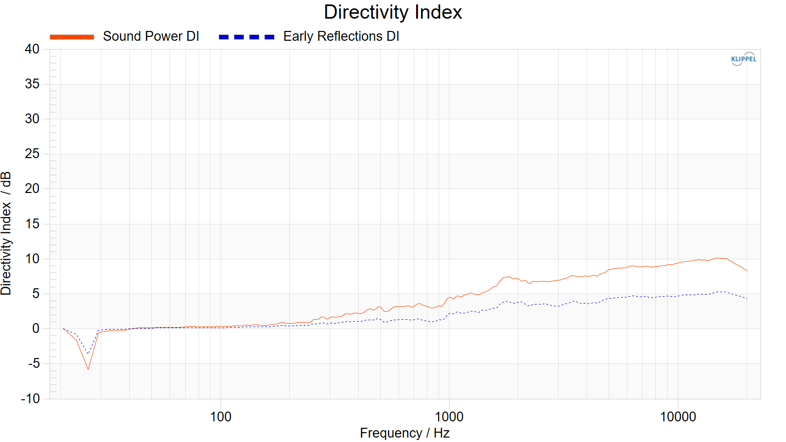
Sound Power Directivity Index (SPDI)

For the purposes of this standard the Sound Power Directivity Index is defined as the difference between the listening window curve and the sound power curve.

Early Reflections Directivity Index (EFDI)

The Early Reflections Directivity Index is defined as the difference between the listening window curve and the early reflections curve.

Early Reflections

The early reflections curve is an estimate of all single=bounce, first=reflections, in a typical listening room. It consists of the following curves:

Floor Bounce

20º, 30º, 40º down

Ceiling Bounce

40º, 50º, 60º up

Front Wall Bounce

0º, ± 10º, ± 20º, ± 30º horizontal

Side Wall Bounce

± 40º, ± 50º, ± 60º, ± 70º, ± 80º horizontal

Rear Wall Bounce

180º, ±90º, ±100º, ±110º, ±120 º, ±130º, ±140º, ±150º, ±160º, ±170º horizontal

According to Devantier: “Characterizing the Amplitude Response of Loudspeaker Systems” AES Convention Paper 5639, 113th Convention 2002

Vertical Reflections

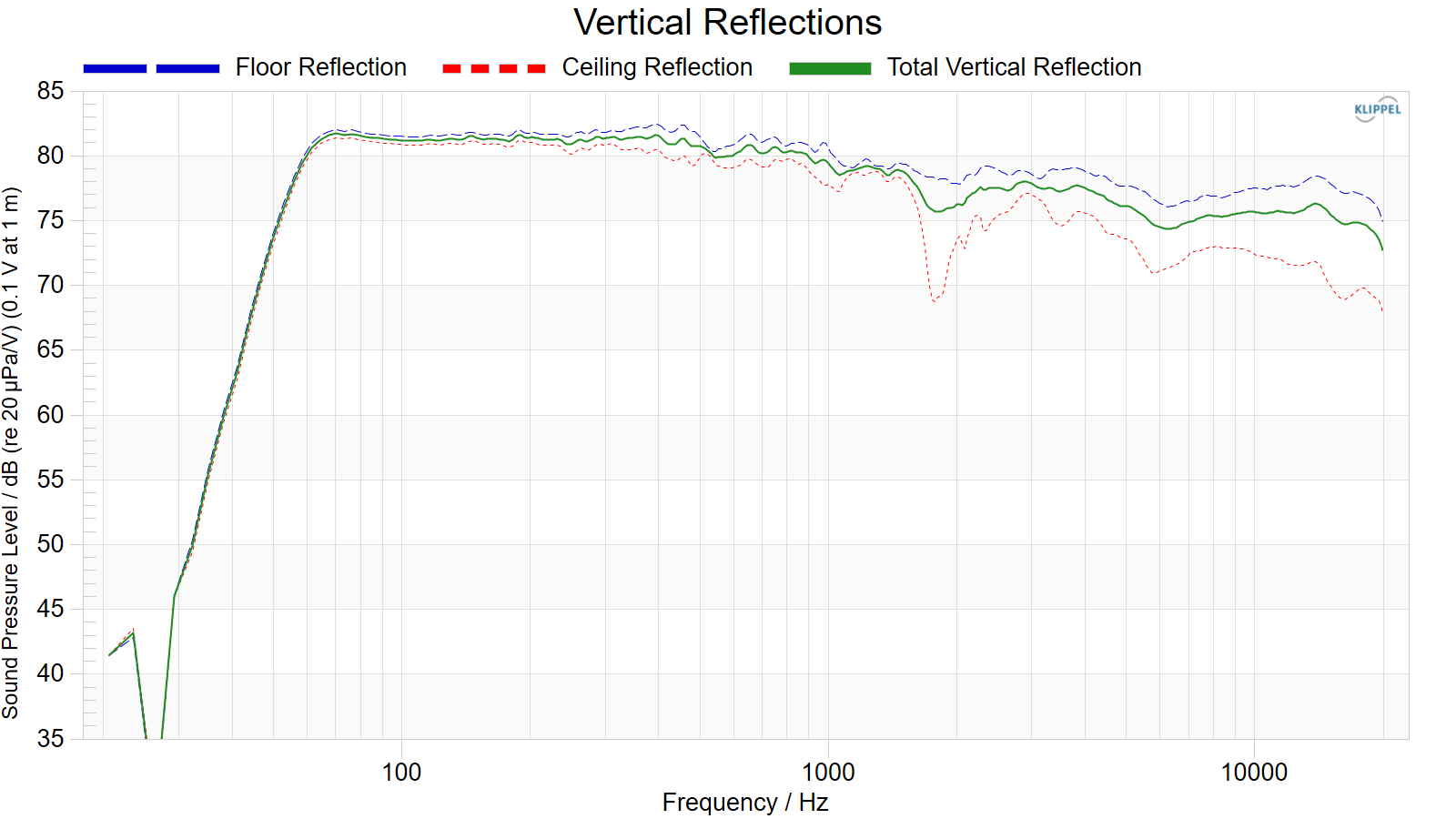
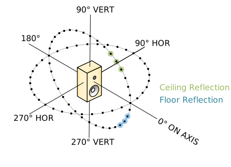
The window summarizes all reflection which are in the vertical radiation plane.

Floor Reflection: 20º, 30º, 40º down Ceiling Reflection: 40º, 50º, 60º up

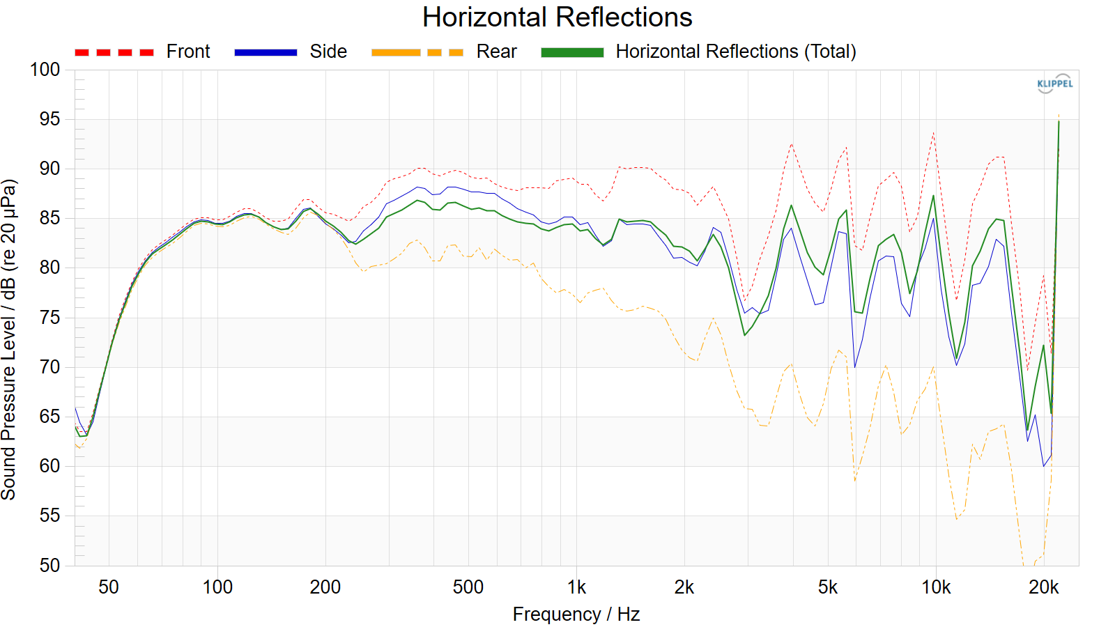
Horizontal Reflections

The window summarizes all reflection which are in the horizontal radiation plane.

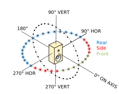
Front

0°, ± 10º, ± 20º, ± 30º horizontal

Side

± 40°, ± 50°, ± 60°, ± 70°, ± 80° horizontal

Rear:

± 90°, ± 100°, ± 110°, ± 120°, ± 130°, ± 140°, ± 150°, ± 160°, ± 170°, 180° horizontal, (i.e.: the horizontal part of the rear hemisphere)

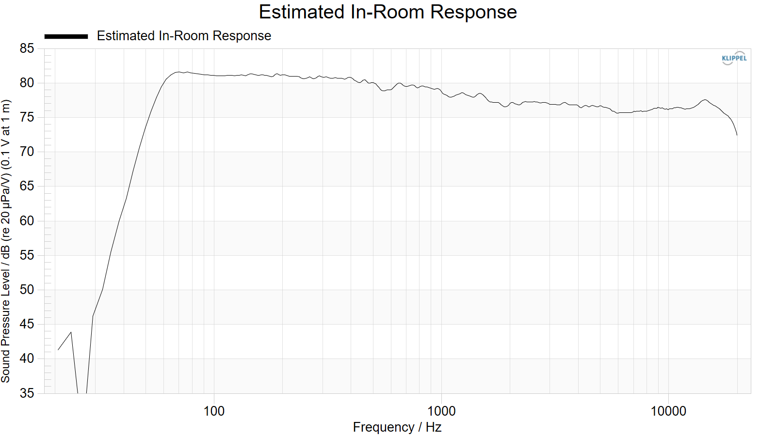
Estimated In-Room Response

The curve estimates the behavior of the loudspeaker in a normal listen room, It is calculates by using a weighted power average with the following configuration:

12% Listening Window, 44%, Early Reflections, and 44% Sound Power.

Directivity Index

Window show the both the Sound power Directivity Index (SPDI) and the Early Reflection Directivity Index (EFDI)

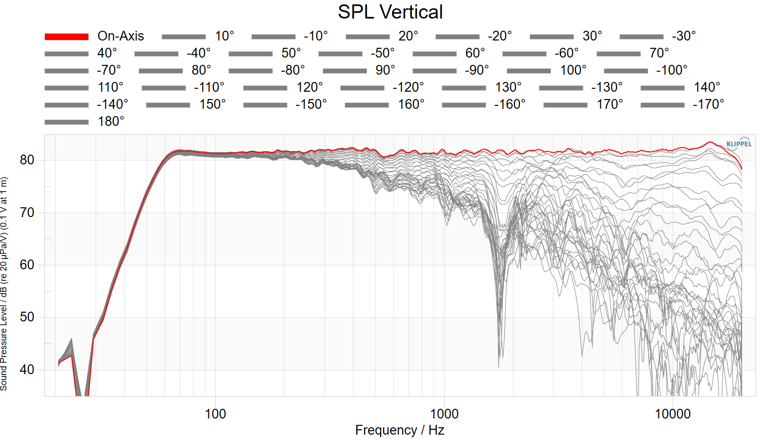
H(f) Magnitude (Vertical)

The window shows all vertical responses which were are used for the CEA2034 calculation.

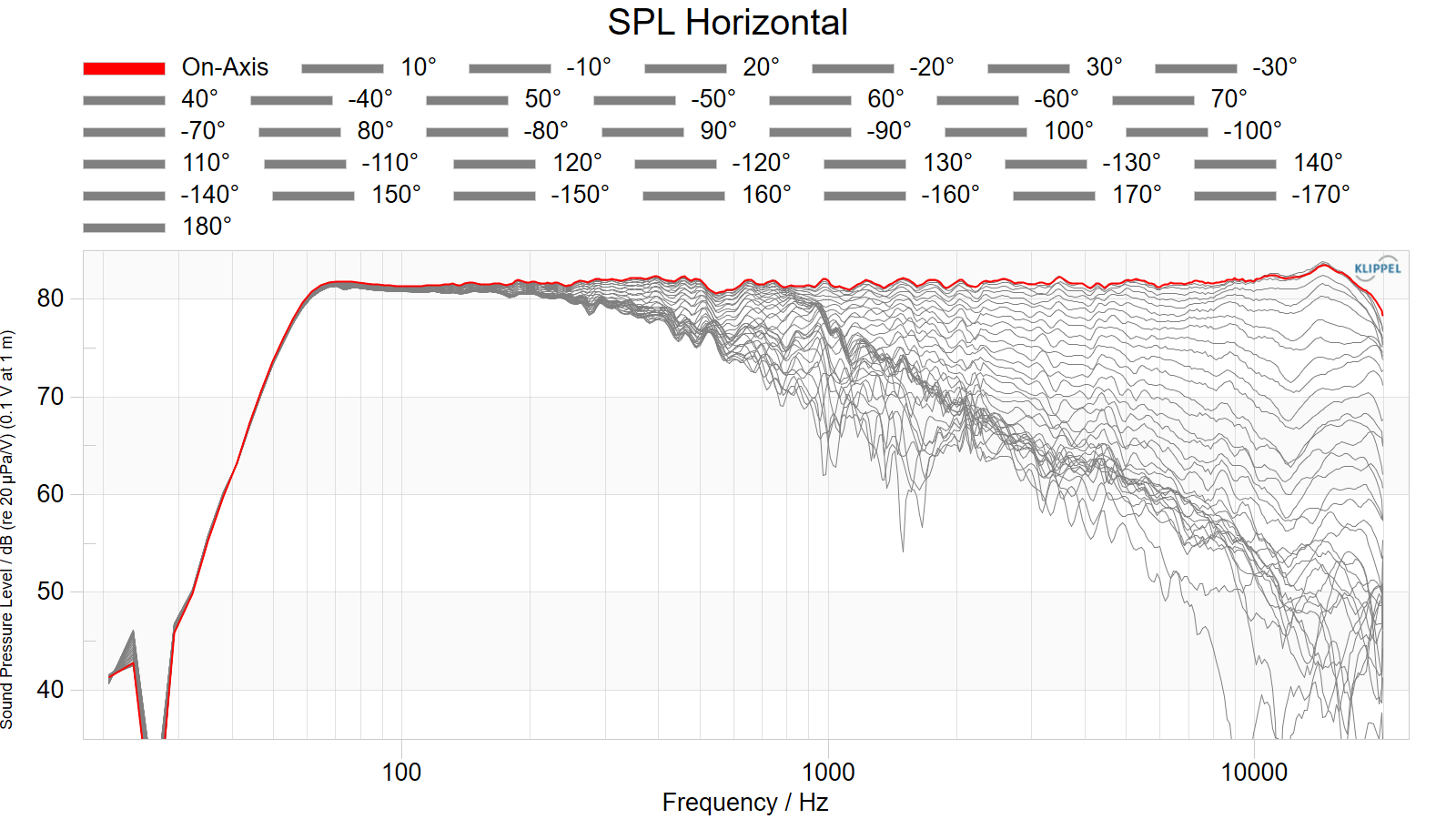
H(f) Magnitude (Horizontal)

The window shows all horizontal responses which were are used for the CEA2034 calculation.

Weighting Table Sound Power calculation

Init Point Concept

During a measurement the measurement equipment or other devices must not be damaged in any way. Therefore, Setting up several setup points enables the definition of a prohibited area or relevant physical information about the measurement device (Figure 16). Presented is a possible setup to perform a cylindrical driving job around a loudspeaker (cylindrical coordinate system with coordinates r, z, φ). The prohibited area is marked in cyan.

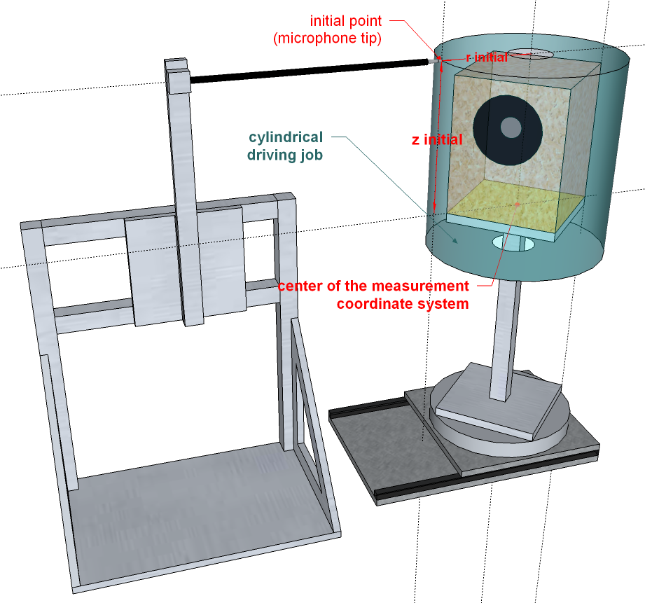
Figure 16: Measurement with initial point and prohibited area

Before the start of the measurement it is the users-task to move the microphone manually to the initial position as shown in the picture. In this case it is the point that is on the upper rim of the cylinder when the microphone faces the loudspeaker at the upper edge.

The values of the additional parameters dim1_init, dim2_init and dim3_init are relayed from the Robotics in the operation MeasurementArray. These values define limits for the r- and z-axis. An example how the measurement range for the z-axis is defined:

Assuming that the z-axis corresponds to dimension 2, the value for dim2_init is identical with z_upper and sets the absolute upper limit for this axis. The relative value z_lower which can be specified by the user in dB-Lab is a value relative to dim2_init. More precise, z_lower defines how much beneath the upper limit lies the lower limit, thus z_lower defines the width of the measurement range. The absolute lower limit can be calculated by subtracting z_lower from the initial dim2_init.

Note

The parameters name_lower do have a different meaning (relative limit instead of absolute limit) when working with an initial point.

The Robotics always saves the coordinates of the initial-point in the “config.ini”-File. So when starting a new measurement, you can either define a new initial-point like it is described above, or use the initial-point of the last measurement (be very careful with that option, especially in cases when the dimensions of the measurement-object changed).

Troubleshooting

Problems with the hardware

There are many possibilities for hardware-related problems. For example connection-problems (hardware could not be found) or mistakes by the user in selecting and parametrizing the hardware.

• Please check all connections between actuators and the computer running the Robotics-Software.

• Try to move each device manually from the hardware-setup-dialog.

• You may also try to use the software from the hardware-developer to control the devices.

Klippel Axis Control

Axis Control connected to another Com-Port

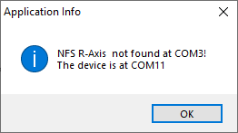
What to do?

Write the correct COM-Port into the “Port./Addr.” field of the Axes.

Axis Control not connected

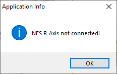
What to do?

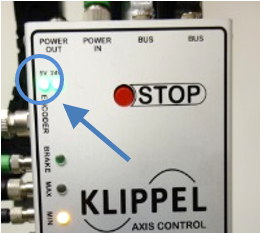
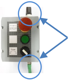
1. Check Power Supply

• Check the 5V and 24V LEDs at the motor boxes. If they are on, everything is OK with the power supply.

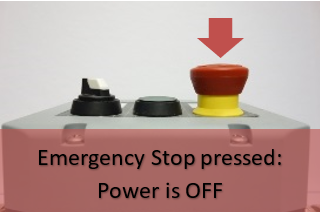
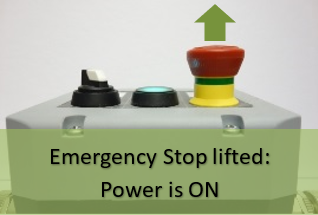
• Check Emergency Stop

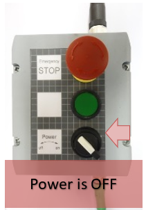
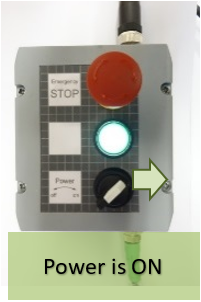
• Check Power Switch

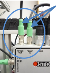
• Check all power connections

2. Check COM-Port

• Check if the devices are assigned correctly.

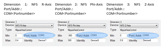
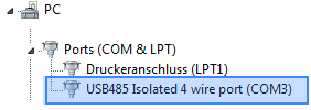
• Check the Windows device manager, which COM-Port has been assigned to the USB-RS485 converter. Use this port number and enter it in the Port/Addr field. (e.g. for COM port 3 enter “COM3” into the Port/Addr field)

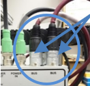
3. Check RS485 Bus connection

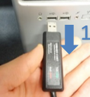
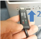
• Reconnect RS485-USB adapter to PC

• Check BUS connection at the motor boxes

Outline ET250

Error Connecting to Outline ET250-3D

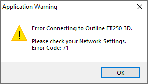
In case the Initialization of the ET250 -3D has failed, please check the following:

1. Is the ET250-3D turned on?

2. Are PC and turntable properly connected via the Ethernet?

3. Is the IP-Address of the turntable correct?

4. Has the Robotics software the access authorization to communicate thru the network? (Maybe ask your network administrator)

What is the IP-Address of the ET250-3D turntable?

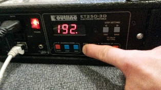
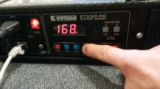
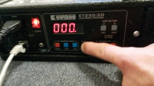
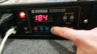
There is a simple way to check the IP-Address of the turntable.

1. Turn off the ET250-3D

2. Push the STOP button and hold

3. Turn on the ET250-3D while holding the STOP button.

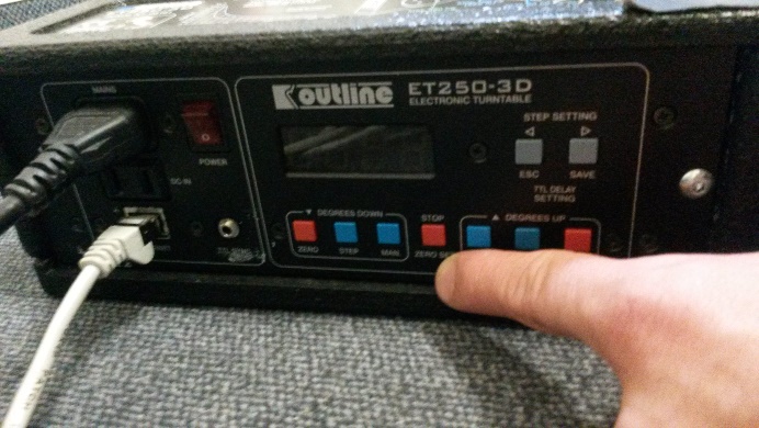
4. During the startup, the display will show the IP-Address of the turntable (e.g. 192.168.0.184)

How to change the IP/MAC Address of the ET250-3D to integrate it in the network?

The IP-configuration can be changed by using the ETcommander2012.exe which is provided from OUTLINE.

1. Run the program ETcommander2012.exe as an Administrator (right click -> Run as administrator)

2. Click Scan Net and select your network interface

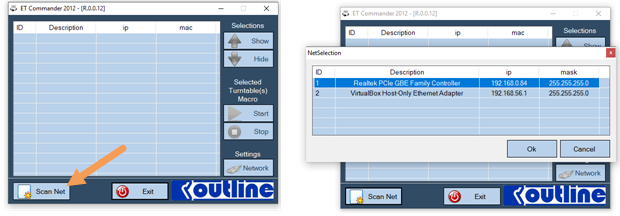
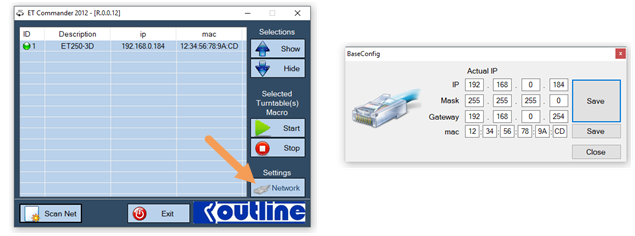
3. After clicking OK, the ETCommander shows the connected turntable in a list.

4. Select the turntable and click Network.

5. Dialog shows up, where the IP and MAC of turntable can be configured.

Usage of multiple ET250-3D turntables

Performing a balloon measurement two ET250 turntables can be used

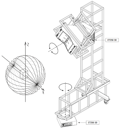
To do this, connect both ET250-3D turntables to the same network and ensure each turntable have a unique Port and IP-Address.

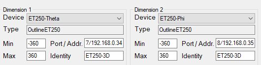
The IP-Address of each turntable can be defined using the ETCommander Software from Outline.

Please also check the MAC-Address of each turntable to avoid conflicts. This can be done with the ETCommander as well.

LinearX Turntable

LinearX LT360 is not connected

Make sure you are using the RS=232 Interface! The Klippel Robotics Software is only supporting the RS232 interface, because the USB-drivers from LinearX are only supporting 32-bit OS.

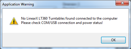
What to do?

• Check power connection of LinearX Turntable

• Check COM-connection of the Turntable

• Check if the cable is correct connected to the Turntable

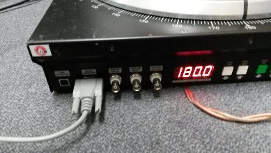
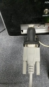
• Check in the device manager if COM connector is available

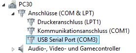
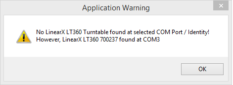
Linear is connected to another port

What to do?

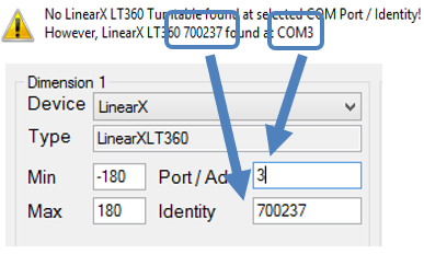
• Read the port and the Serialnumber from the messagebox.

• Insert the correct Port and Serialnumber into the Hardware Setup

Problems with the Robotics-Software

In the unlikely event the Robotics-Software itself crashes, please make a screenshot of the error and send it to Klippel GmbH. Also always attach the Robotics.log.

Problems with dB-Lab

There are many possibilities for dB-Lab-related problems. For example: problems with the database, problems with the automation-interface and so on. A good start for troubleshooting these problems could be:

• Start dB-Lab-Software manually

• Open the same database, you want to process with the Robotics

• Try to start the measurement-operation(s) manually to see if they are configured correctly.

License problems

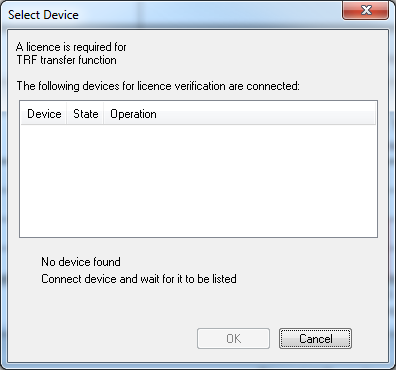
When there is a license missing, you will get an error-message from the dB-Lab-Software in which you can easily recognize which license for which device is missing. Make sure you have valid licenses for the correct dB-Lab-Version. If you need new licenses, please contact Klippel GmbH.