ISC – In-Situ Room Compensation

ISC – Tutorial

Principle

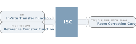
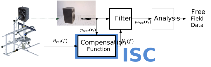
The In-Situ Room Compensation is a processing module that calculates complex filter functions to compensate for the influence of a non-anechoic measurement environment. This filter is the key to perform accurate acoustic measurements in almost every environment and to determine accurate free field frequency responses and non-linear symptoms (e.g. harmonic distortion, intermodulation distortion, thermal compression, etc.)

Viewing Results (Part 1)

Example data used in this manual is stored in the Web Example database. If not downloaded already, get it from the latest R&D release <https://www.klippel.de/go/current-rnd-release> and open the web-based database.

See also

View Results for general information on how to download this database, open and view results in dB-Lab.

Select in the folder Directivity + Room Correction (NFS, ISC, POL) the driver object Room Compensation - Subwoofer (ISC, TBM, TRF, NFS)

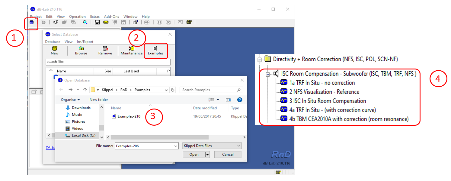
This object shows the results of subwoofer measurement. The target is to measure harmonic distortion with the TRF – Transfer Function Measurement module and the CEA 2010 maximum peak SPL using the TBM – Tone Burst Measurement module. All measurements are performed in a normal office room.

Measurement in Room (no compensation)

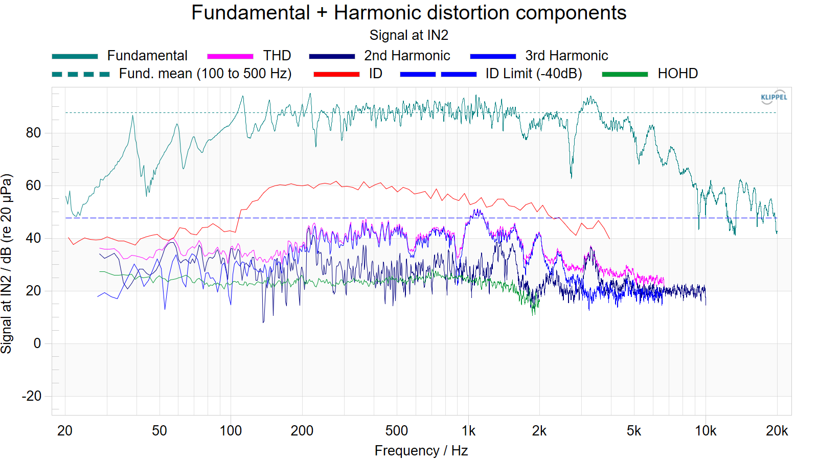
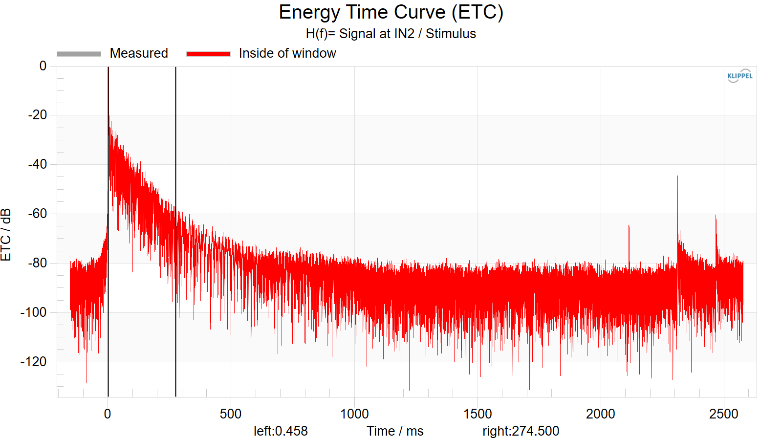
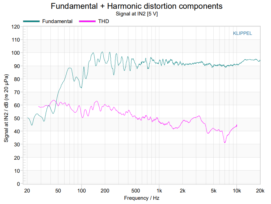
Open the operation 1a TRF In Situ – no correction and select the result window Fundamental + Harmonics. The Fundamental response shows very distinct room modes at low frequencies (below 300 Hz). These resonances, which change the SPL by ±10 dB, make an accurate acoustical measurement impossible. The Energy Time Curve shows the decay of the room very clearly. The sound pressure decays slowly. It takes about 500 ms until the sound pressure decay amounts to -70 dB. The harmonic distortions are showing this decay as well, because they are post filtered by the same room impulse response.

Note

Always ensure that the microphone is calibrated correctly before performing an acoustic measurement. See also Sensor Handling

In the following the ISC module will be used to compensate for the room influence.

Reference Measurement

To determine the compensation filter of the room a reference measurement is required. In this example the speaker was measured with the NFS – Near Field Scanner, which gives very accurate free field data. The Operation 2 NFS-Reference shows the free field frequency response of the speaker.

There are other methods to determine the low frequency reference of a speaker as well. For example the device can be measured in a good anechoic room or outside in free field. In addition, while considering the specific limitations and assumptions also a near field measurement or a simulation based on lumped parameters can be used to determine the reference SPL response.

Compensating the Room

Select the operation 3 ISC In Situ Room Compensation and open the Property Page.

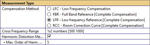
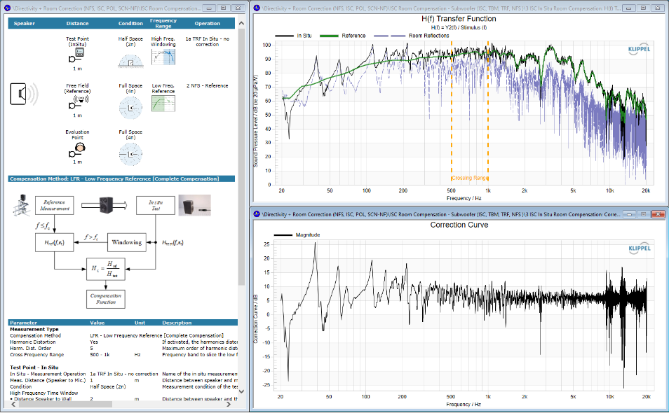
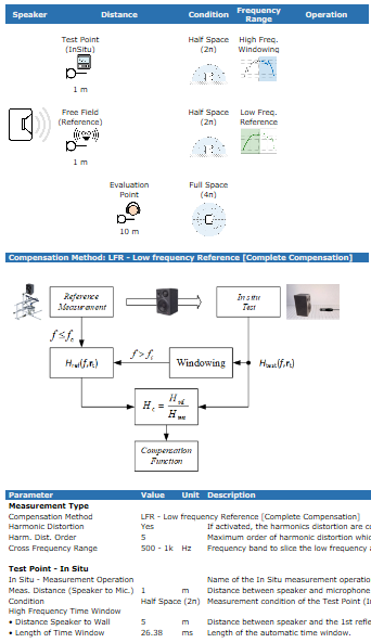
The example uses the LFR method (Complete compensation with Low Frequency Reference), which requires only a low frequency reference and uses a time windowing to determine the high frequency free field response. For more details see the section ISC - Reference.

The transition range between windowing and the low frequency reference is defined by the parameter Cross Frequency Range.

In addition, there is a parameter to exclude or include the harmonic distortion of the In-Situ Measurement from the compensation filter. Here, Harmonic Distortion Measurement is checked to keep the distortion and don’t compensate for it.

The next categories are specifying the source data for the ISC module. Both the In-Situ and the Reference measurements are linked as operation. In this example the measurement distance of the Free Field Reference and the test point are identical, but the In-Situ TRF – Transfer Function Measurement was measured under half space condition which causes 6 dB more output. This difference can be compensated automatically by selecting the automatic adjustment of Distance + Meas. Condition in the section Transfer Function Adjustments using the parameter Gain Adjustment.

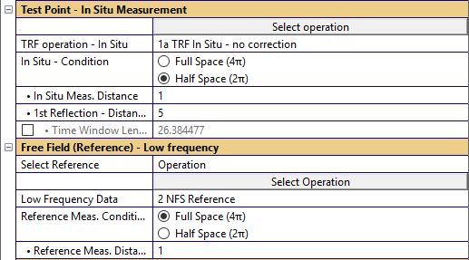
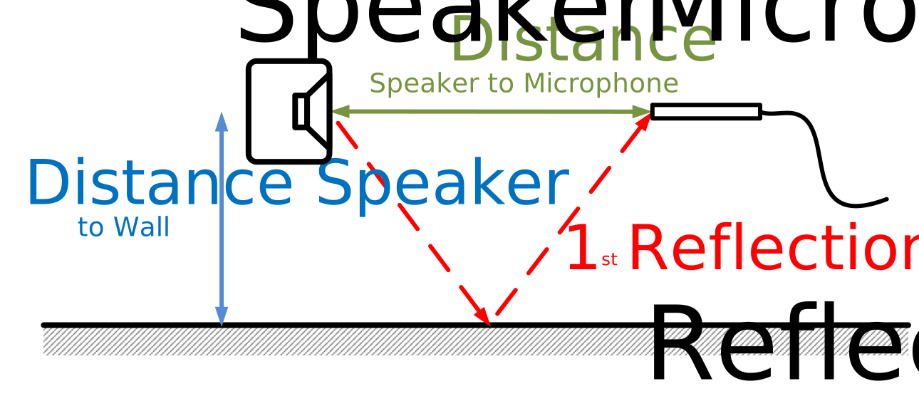
The LFR method has an additional section to specify the time window for the high frequencies. The module uses a Tukey window with an alpha parameter set to 0.5. The length of the window can be defined by hand or calculated automatically based on the distances to the room boundary and to the microphone.

The next category includes the automatic adjustments of the transfer function. These adjustments are useful to correct small mismatches between the Reference measurement and the In-Situ measurement, e.g. a delay mismatch caused by small positioning errors.

After running the ISC all parameter and automatic adjustment or mismatches are shown the Summary window. Also the frequency responses or the source data and the final compensation function are visualized in result windows. Using the Display tab of the Property Page, further information e.g. Phase Response can be shown.

Step-by-Step Tutorial (Part 2)

This tutorial explains how to perform a standard acoustic measurement in a non-anechoic environment using the ISC module. The workflow is demonstrated using a passive 2-way loudspeaker system measured in a normal office environment. The loudspeaker operates full range and is mounted in a vented enclosure.

The Low Frequency Reference (LFR) method is applied, using the Near Field Scanner (NFS) as the reference measurement system. The Near Field Scanner provides an accurate free-field reference at low frequencies, which is required for the room compensation process.

The main focus of this tutorial is the application of the room compensation function. Detailed instructions for performing the Near Field Scanner measurement itself are not covered here and are described in detail in the NFS section.

Step 1: Reference Measurement Using NFS

The reference measurement is carried out with the NFS in a standard office environment. Since the LFR compensation method requires low-frequency reference data only up to approximately 1 kHz, the sound field remains relatively simple. A coarse scan with around 100 measurement points and a total measurement time of approximately 15 minutes is therefore sufficient.

After completing the scan, all data is automatically stored in a predefined measurement template. The Measurement Data Container includes the spatial coordinates of the measurement points, the recorded impulse responses, and additional meta-information describing the measurement setup. The measurement grid is visualized to verify proper spatial coverage of the sound field.

The acquired data is then processed using the NFS Field Identification operation. This step applies standard signal processing followed by the identification of the sound field coefficients. The fitting error is evaluated to confirm that the selected expansion order and the number of measurement points are adequate for accurate sound field reconstruction.

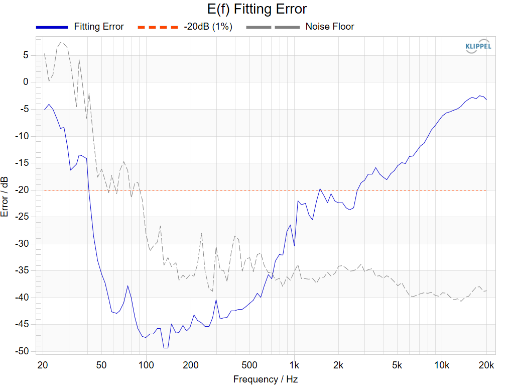
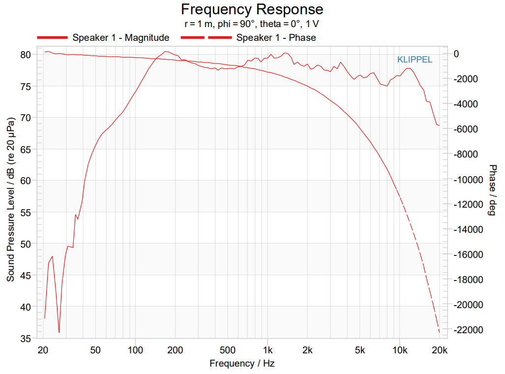
In the final step, the NFS Visualization is used to extrapolate the measured sound field to free-field conditions. A 1 meter on-axis frequency response is extracted and used as the low-frequency reference for the ISC process. Small noise-related irregularities below approximately 40 Hz are not critical for further processing.

Step 2: In-Situ Measurement Setup

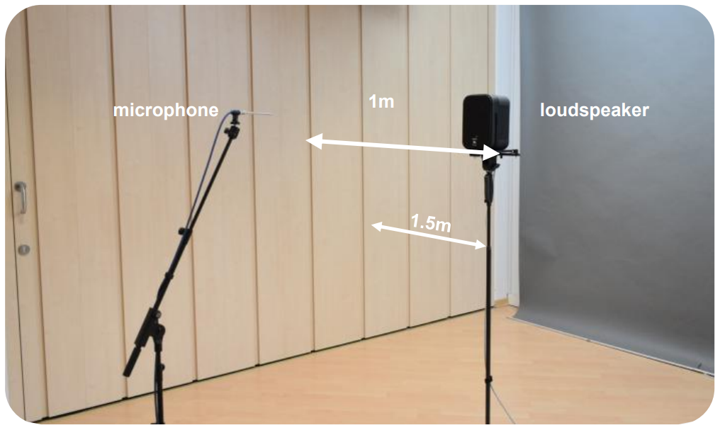
The In-Situ measurement captures the loudspeaker response under real room conditions. To delay the first room reflections as much as possible, both the loudspeaker and the microphone are placed in the center of the room. The microphone is positioned 1 meter on-axis from the loudspeaker. In rooms with a low ceiling and large floor area, ground-floor measurements can be beneficial.

The ISC object template consists of three main operations. First, the low-frequency reference obtained from the NFS Visualization is defined. Second, a TRF In-Situ measurement is performed using a logarithmic sweep. Finally, the ISC In-Situ Room Compensation operation calculates the complex compensation filter that removes the influence of the room.

Step 3:TRF In-Situ Measurement

The TRF In-Situ module is used to measure the transfer behavior of the loudspeaker, including the fundamental frequency response, harmonic distortion, and time-domain responses. Measurement settings can be adapted to the specific application, as described in the TRF Manual.

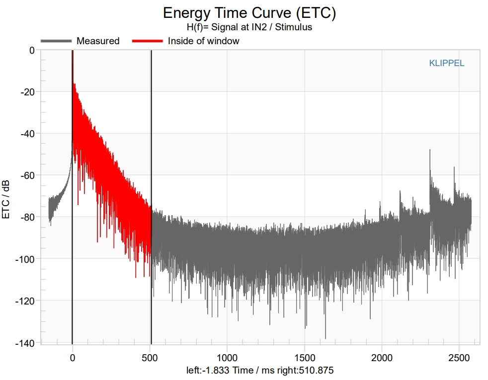
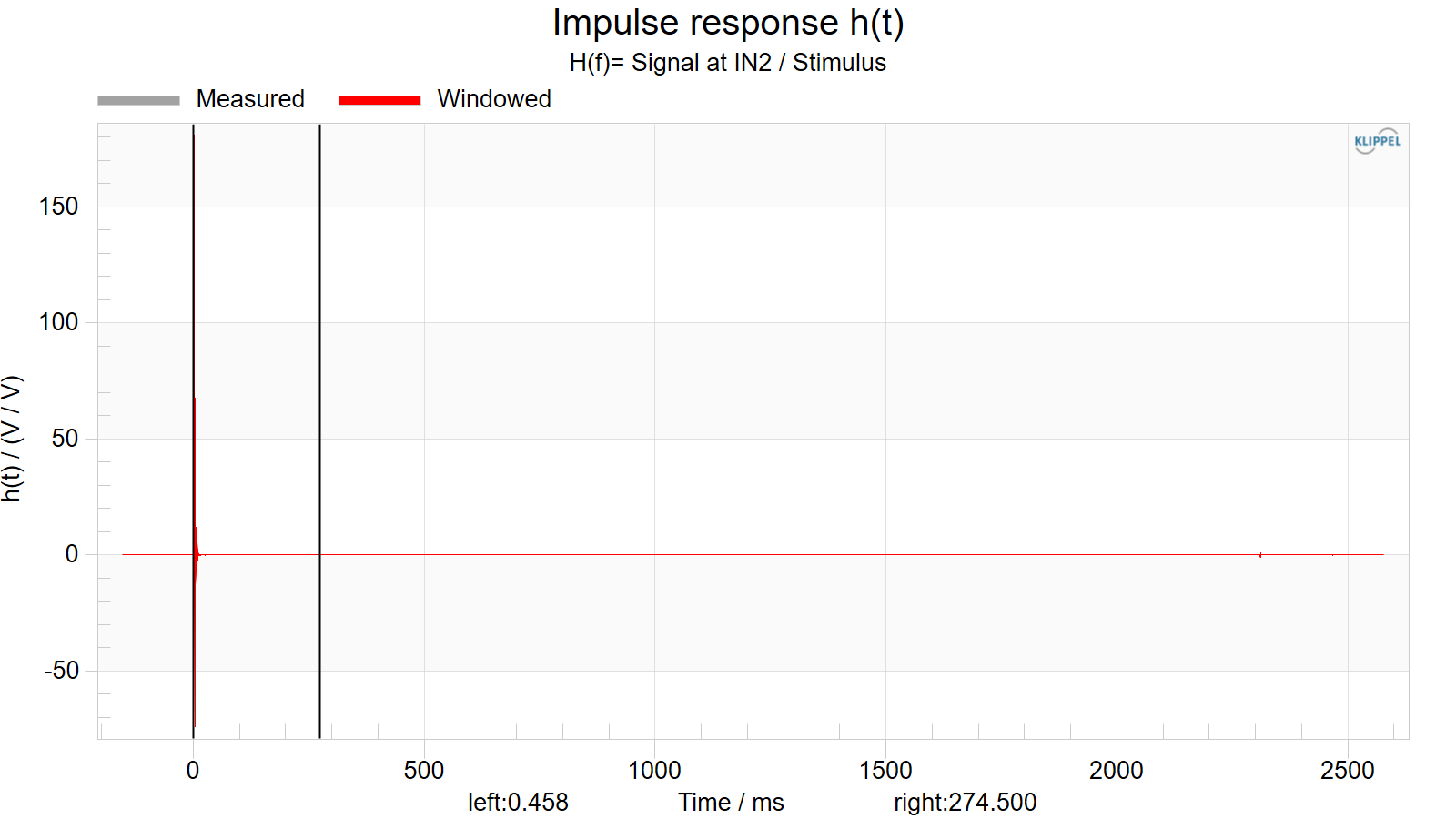
Without compensation, the impulse response shows a long decay of approximately 500 milliseconds, and early room reflections are clearly visible. The reverberation strongly affects the separation of harmonic distortion components. In the frequency domain, room modes dominate the response below about 500 Hz, resulting in strong peaks and dips exceeding 10 dB. Harmonic distortion measurements are therefore heavily influenced by room effects.

Note

The following guidelines should be considered when performing in-situ measurements:

• Ensure that the Signal-to-Noise Ratio (SNR) is at least 40 dB.

• Make sure that the Impulse Response (IR) duration is sufficiently long to capture the complete decay of the room accurately.

Step 4: ISC Setup and Configuration

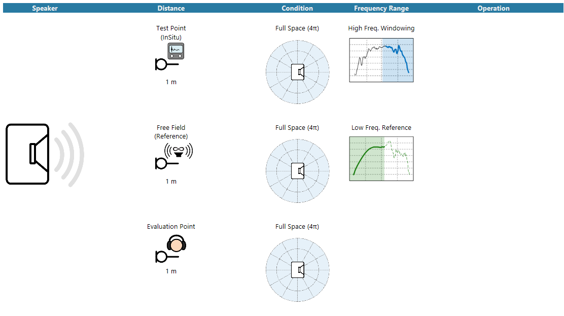
The ISC configuration defines three positions: the test point where the In-Situ TRF measurement was performed, the free-field reference position obtained from the NFS measurement, and the evaluation point where the final results are mapped. In this example, all three points are defined at the same position at 1 meter on-axis. However, different positions can be used if near-field effects need to be compensated.

The ISC property page is configured according to the application. The LFR method is selected, which combines a low-frequency free-field reference with a time-windowed high-frequency response. The cross frequency range is set between 500 Hz and 1 kHz, where both responses are merged and validated. Harmonic distortion measurement is enabled to ensure that non-linear components are not compensated and remain physically meaningful. Default transfer function adjustment settings are used to correct small mismatches, such as minor delay errors caused by positioning inaccuracies.

Step 5: ISC Results and Verification

After running the ISC operation, a complex correction filter is generated. This filter compensates the influence of room reflections and resonances and can be applied to further acoustic measurements.

In the frequency domain, the uncorrected In-Situ measurement shows variations of more than 20 dB caused by the room. After compensation, the frequency response becomes smooth and closely matches the free-field reference. In the time domain, the compensated impulse response shows that the long room reverberation has been removed, leaving only the short decay of the loudspeaker. Room reflections are also effectively removed from the distortion components.

The corrected harmonic distortion results demonstrate that the compensation filter works consistently for both linear and non-linear responses, enabling accurate evaluation of the loudspeaker behavior.

To verify the calculated compensation filter, the In-Situ measurement can be repeated using a different microphone position while keeping the measurement distance constant. Without compensation, the results show significant deviations. After applying the compensation filter, consistent frequency response and harmonic distortion results are obtained. An example of this verification process is available in the Klippel ISC demonstration video.

Measurement with various Stimuli (TRF, TBM, MTON, DIS) (Part 3)

The compensation function, calculated by the ISC-Module, is dependent on the physical measurement setup, speaker and microphone position, but is independent on the stimulus. That means the filter can be also applied to various other measurements (steady state or transient e.g. TRF – Transfer Function Measurement, DIS – Distortion, MTON – Multi-Tone Measurement, TBM – Tone Burst Measurement).

Transfer function Measurement (TRF)

ISC Module is creating automatically a copy of the TRF In-Situ operation that has the compensation filter applied.

Open the operation 4a TRF In Situ (with correction curve). The Impulse Response shows that the long decay of the room was removed. Also the distinct room modes can be compensated by the filter. The room effects are removed from the fundamental as well as from the harmonics, thus a valid and accurate Harmonic Distortion measurement can be performed.

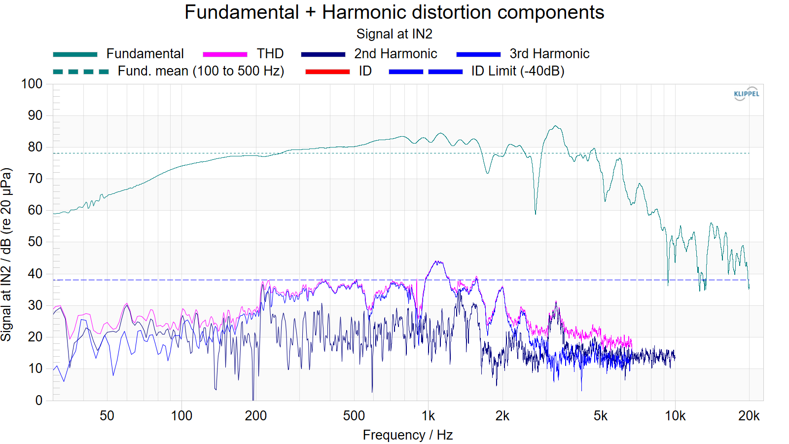
For further harmonic distortion measurement with the TRF module this operation can be used as a template.

Tone Burst Measurement (TBM)

Performing burst tests on subwoofers in compliance with CTA-2010 and CTA-2023 standards poses challenges, particularly due to room modes, which are critical issues in the low bass range (f < 100 Hz). Finding an environment suitable for accurate measurements in this frequency range is nearly impossible.

However, room imperfections can be compensated for effectively using a correction filter. Follow these steps to apply the correction filter:s.

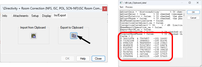
1. Export the Filter Curve from ISC-Module

Use the Clipboard Export function of the ISC Module to export the correction filter curve.

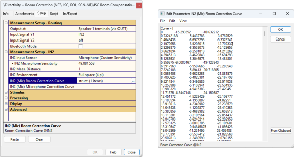
2. Apply Correction Curve to TBM microphone settings

Apply the exported room correction filter to the microphone using the In1(Mic) Room Correction Curve or In2(Mic) Room Correction Curve parameter.

3. Start the TBM measurement

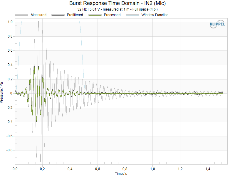
Open the operation 4b TBM CEA2010A with correction (room resonance). This example demonstrates a TBM measurement conducted in a typical office room, where the microphone response is filtered using a compensation curve generated by the ISC Module.

Open the graph y1(t) Waveform. The curve Measured is showing the original signal of the microphone. The burst fundamental frequency was close to a room resonance and the short tone inputs enough energy to excite this low damped resonator. After applying the compensation filter (curve Prefiltered) the resonance was almost completely removed and a valid acoustical measurement was performed.

Multi-Tone Measurement (MTON)

In order to use a room correction for the MTON module, the following steps must be taken:

1. Export the Filter Curve from ISC-Module

Use the Clipboard Export function of the ISC Module to export the correction filter curve.

2. Apply Correction Curve to MTON microphone settings

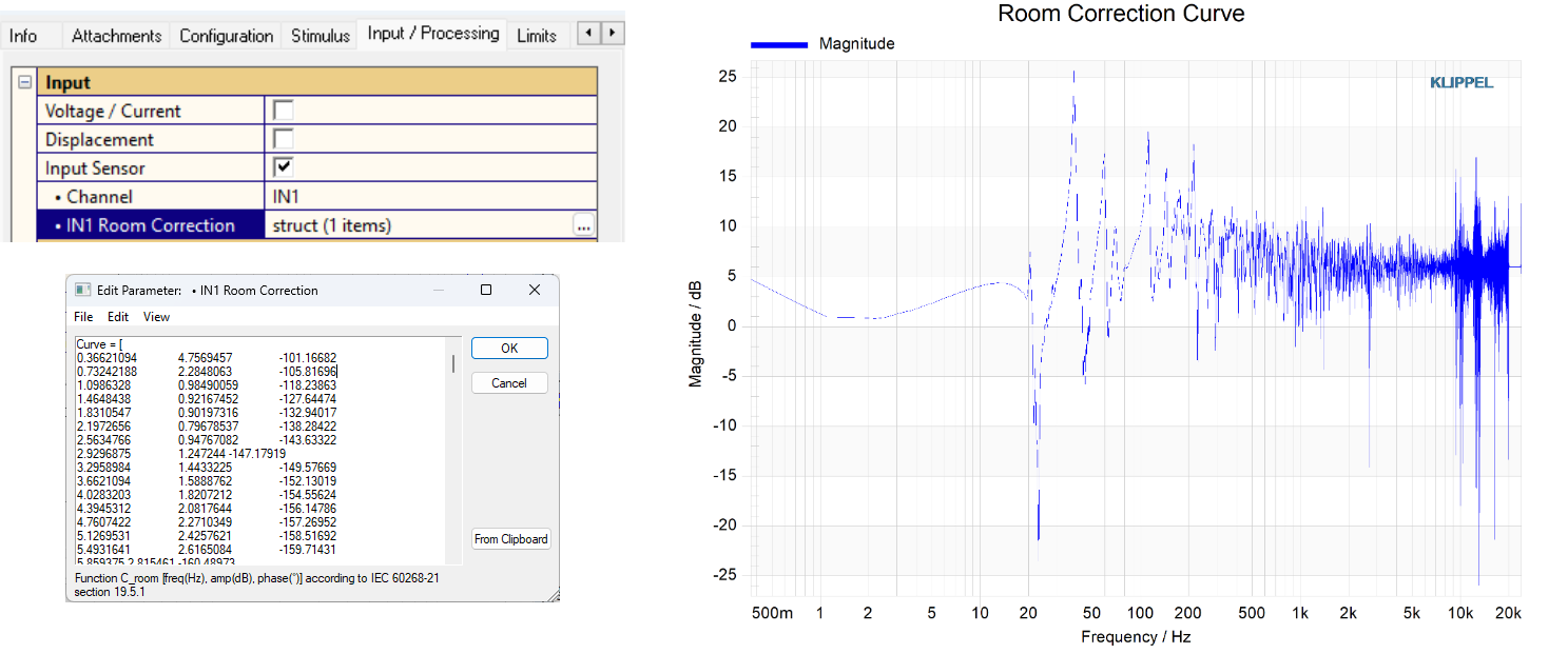
Apply the exported room correction filter to the microphone using the IN1 Room Correction parameter. The imported correction curve is displayed in the Room correction Curve result window.

3. Start the MTON measurement

During the processing the microphone signal is automatically filtered by the correction curve to ensure valid and accurate measurements.

3D Distortion Measurement (DIS)

In order to use a room correction for the DIS module, the following steps must be taken:

1. Export the Filter Curve from ISC-Module

Use the Clipboard Export function of the ISC Module to export the correction filter curve.

2. Apply Correction Curve to DIS microphone settings

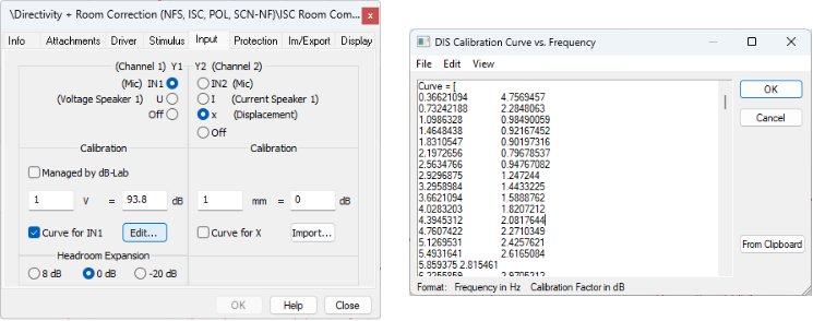
Use the calibration curve of the microphone input to consider the correction curve for you distortion measurement.

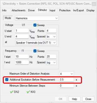
Also set an additional excitation before the measurement to ensure that everything in steady state. The time depends on the decay of the room.

ISC - Reference

Parameters

Measurement Type

Compensation Method

Selection of the method that is used to calculate the compensation filter.

Low Frequency Compensation (LFC)

Features

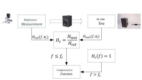
• requires accurate reference response \(H_{\mathrm{ref}}(f,\textbf{r}_{\mathrm{r}})\) with sufficient resolution at low frequencies only (below 1 kHz)

• compensation function \(H_{\mathrm{c}}(f)\) is valid for a wide range of speakers

• microphone positioning error has small influence on compensation function

Limits

• Requires good acoustic treatment of the measurement room for high frequencies (above 1 kHz)

• measurement points r_r and r_t shall be identical

• distance correction assuming far field conditions (\(1/r\) law)

Application

• Measurement in small (bad) anechoic room

• Calculating a generic room correction curve for a fixed setup

Complete Compensation with Full Band Reference (FBR)

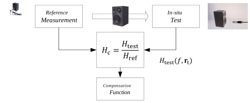
Features

• compensates for different measurement points r_r and r_t

• compensation of room influence, position of the measurement points (e.g. near field effects)

Limits

• requires accurate reference response \(H_{\mathrm{ref}}(f,\textbf{r}_{\mathrm{r}})\) with sufficient resolution at all frequencies

• microphone positioning error affects the compensation function \(H_{\mathrm{c}}(f)\)

Application

• measurement in small undamped room (e.g. office)

• Far field correction of near field measurements

• Comparison of measurements from different test boxes (e.g. EoL-Test)

Complete Compensation with Low Frequency Reference (LFR)

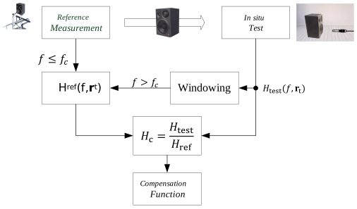
Features

• reference response \(H_{\mathrm{ref}}(f,\textbf{r}_{\mathrm{r}})\) with sufficient resolution at low frequencies only

• compensation function \(H_{\mathrm{c}}(f)\) represents interaction between speaker and room

• microphone positioning error has small influence on compensation function

Limits

• windowing requires sufficient distance from reflective surfaces

• measurement points r_r and r_t shall be identical

• distance correction assuming far field conditions (\(1/r\) law)

Application

• Measurement non-anechoic rooms (e.g. workshop, office)

Room Correction Curve (RCC)

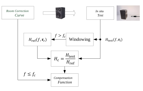
Features

• no reference measure needed

• using a low frequency room correction function

• microphone positioning error has small influence

Limits

• general reference curve only valid for the same measurement position and similar speaker

• measurement points r_r and r_t shall be identical

• distance correction assuming far field conditions (\(1/r\) law)

Application

• Measurement in small (bad) anechoic room

• Calculating a generic room correction curve for a fixed setup

• Measurement non-anechoic rooms (e.g. workshop, office)

Comparison between the Compensation Method

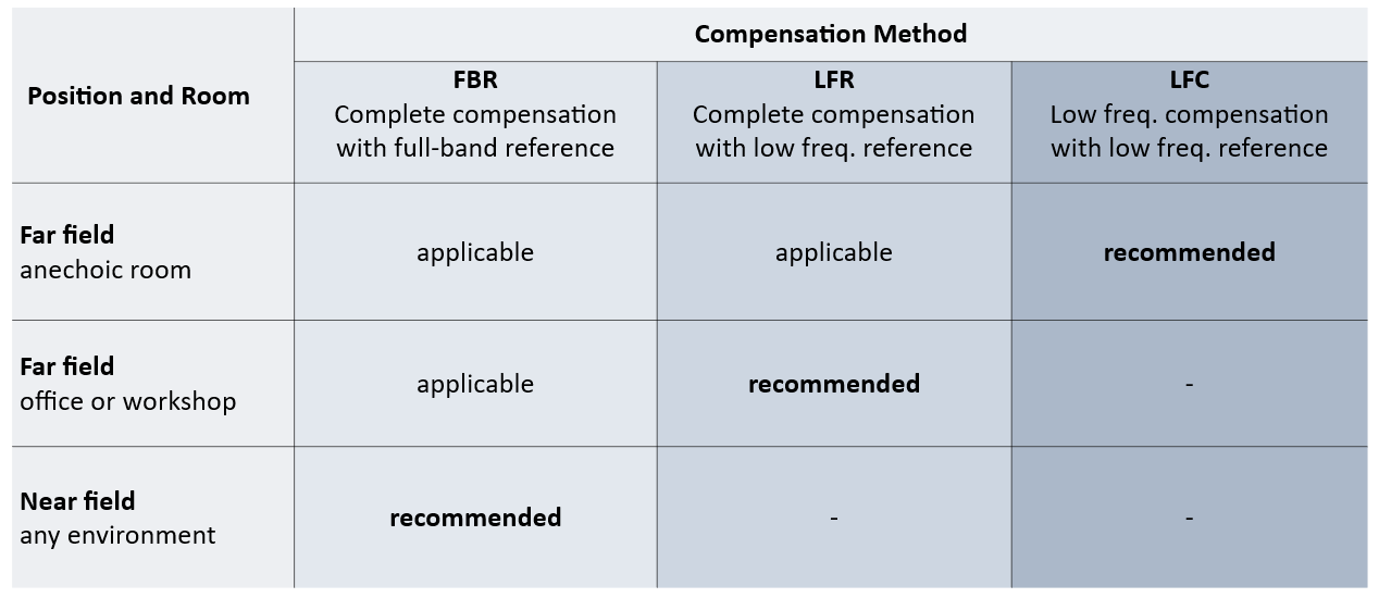
The compensation function is based on a reference, that should be selected depending on the complexity of the device under test. For a simple system like a closed box, near field measurement is a very common way to correct low frequencies. A more advanced measurement system (e.g. Near Field Scanner) is required for more complex sound sources to enable accuracy and flexibility with less assumptions.

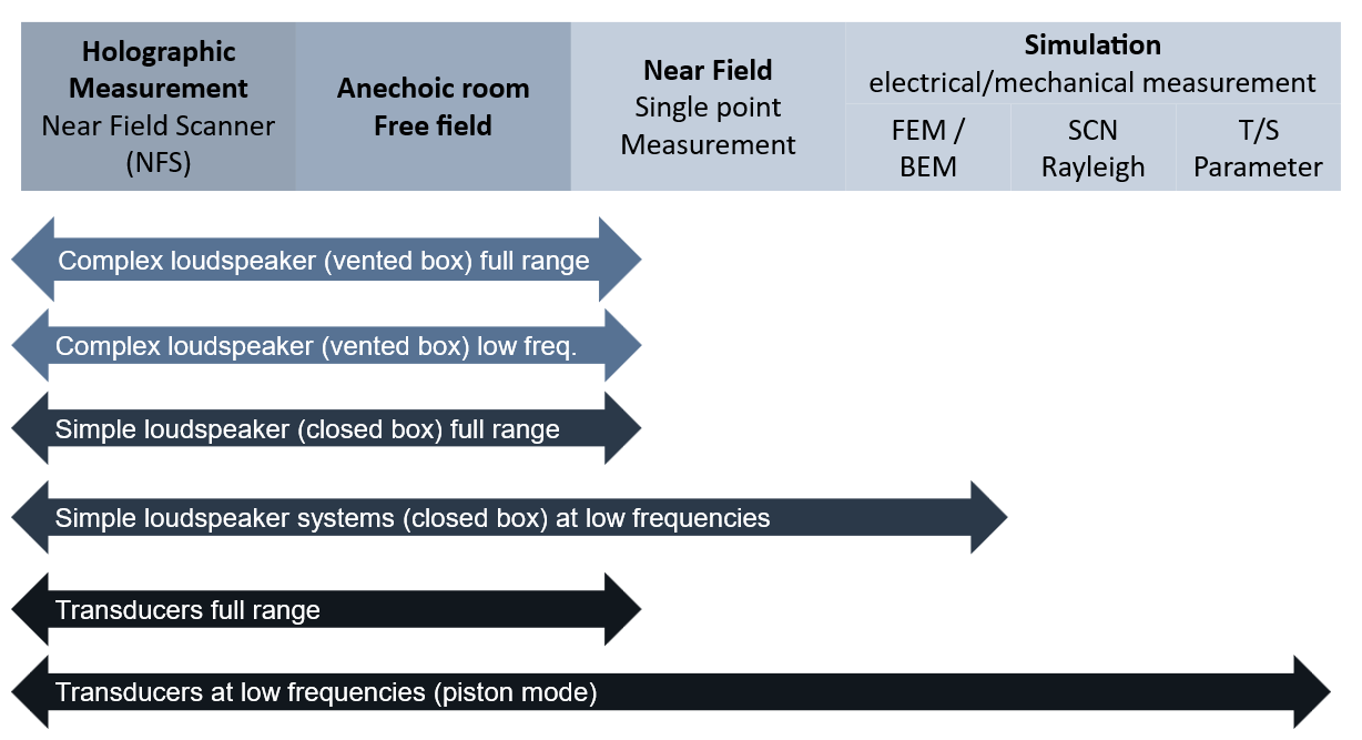
In summary, the table below provides a comparison of the methods described above. Further details can be found in the this paper Fast Loudspeaker Measurement in Non-Anechoic Environment.

Harmonic Distortion Measurement

When using a compensation filter for a harmonic distortion measurement, it is import to compensate only for the fundamental component of the room. This can be done automatically in the ISC by activating the Harmonic Distortion Measurement checkbox and specify the Maximum Order of Harmonic Distortion. Up to this order the harmonic distortion will be included in the measurement with compensation.

Cross Frequency Range

In the Cross Frequency Range the low frequency and high frequency reference curves will be merged to determine a full band compensation curve. The parameter defines the minimum and maximum frequency of this range.

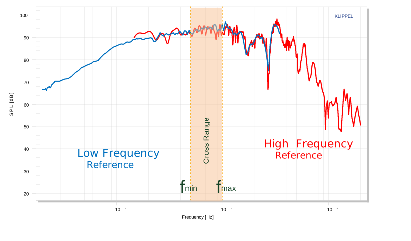
Using a Complete Compensation with Full Band Reference (FBR) this range is only used to do checks and adjustments of the transfer function.

Test Point - In Situ Measurement

Link to the In-Situ TRF operation, which is measured at the Test point. The ISC imports data automatically from the selected TRF operation

In Situ - Condition

The parameter defines if the in situ measurement is performed in a half space or full space setup. This condition will be considered in the automatic adjustment of the transfer function.

Time Windowing

Using the Complete Compensation with Low Frequency Reference (LFR) or the Low Frequency Room Correction curve (RCC), the ISC module is applying an automatic time windowing to separate the direct sound from the room reflections for high frequencies.

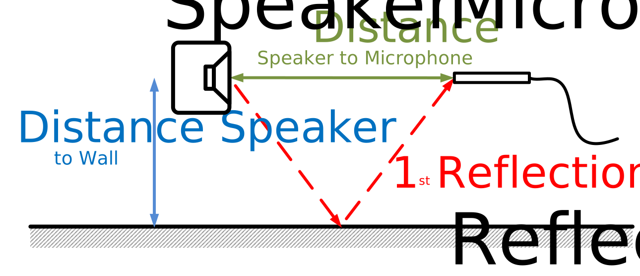
In Situ Meas. Distance

\(d_{sm}\) in \(m\)

Distance between loudspeaker and microphone

1st Reflection - Distance to Wall

\(d_{sw}\) in \(m\)

Distance between loudspeaker and first reflecting wall, used for automatic calculation of the time window length

Time Window Length

\(T_W\) in \(ms\)

Parameter specifies the length of the time window. This can be defined manually or can be calculated automatically by specifying the measurement distance and the distance to the first reflecting wall.

Time Delay

\(\tau\) in \(ms\)

Parameter specifies the time delay of the In Situ impulse response and affects the position of the automatic time window. If the parameter is unchecked the time delay is detected automatically.

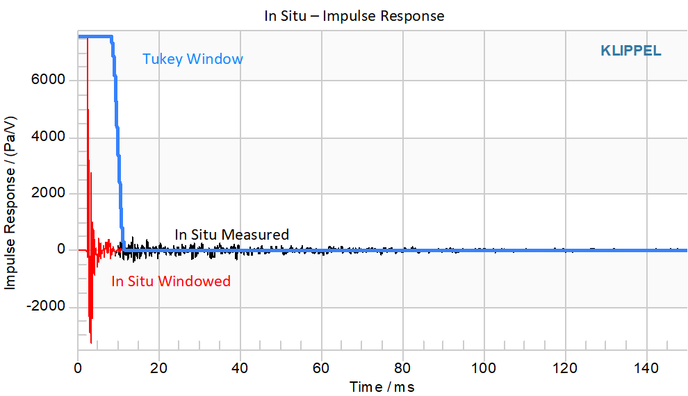
The ISC module is using a Tukey window which is shown in h(t) Impulse Response result window.

Free Field (Reference)

Definition of free field reference curve. This curve can be imported via the Clipboard or by a direct operation link to either a TRF operation measured in free field or to a NFS Visualization operation.

Reference Meas. Condition

The parameter defines if the reference measurement was performed in a half space or full space setup. This condition will be considered in the automatic adjustment of the transfer function.

Reference Meas. Distance

The parameter defines the measurement distance of the reference measurement. This distance will be considered in the automatic adjustment of the transfer function using the 1/r law.

Evaluation Point

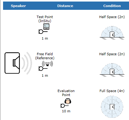
According to the IEC 60268-21 a compensation curve can be used to do an adjustment of the distance and map the data to a specific evaluation point. The ISC module can scale automatically the level and propagation delay using the \(1/r\) law. In addition, the measurement condition e.g. half space or full space can be scaled as well.

The Evaluation Point can be set to

• Test Point,

• Free Field (Reference) Position

• User defined distance.

Differences between Test Point and Evaluation Point and the corresponding scaling are visualized in the summary result window.

For example, if the result should be scaled from a Test Point in 1 m in half space to an evaluation point in 10 m in fullspace.

The ISC module will subtract -26 dB. 20 dB for the distance (\(1/r\)) and 6 dB for the half space full space conversion.

Transfer Function Adjustment

When comparing a reference measurement with an In-Situ measurement, there are usually small mismatches in the mechanical alignment of the measurement setup.

These little mismatches like gain, delay and polarity are checked automatically and can be adjusted to ensure valid compensation filters.

Display

Display parameter for hiding and showing additional results (e.g. phase response)

Results

Summary

The Summary window lists all input parameters of the module, as well as the automatic adjustments and mismatches between the In-Situ and Reference measurement. In addition, warnings and errors will be propagated here.

h(t) Impulse Response

Impulse Response of the In-Situ Measurement. Using the Complete Compensation with Low Frequency Reference (LFR) the automatic time window and the windowed Impulse Response are shown in this graph as well.

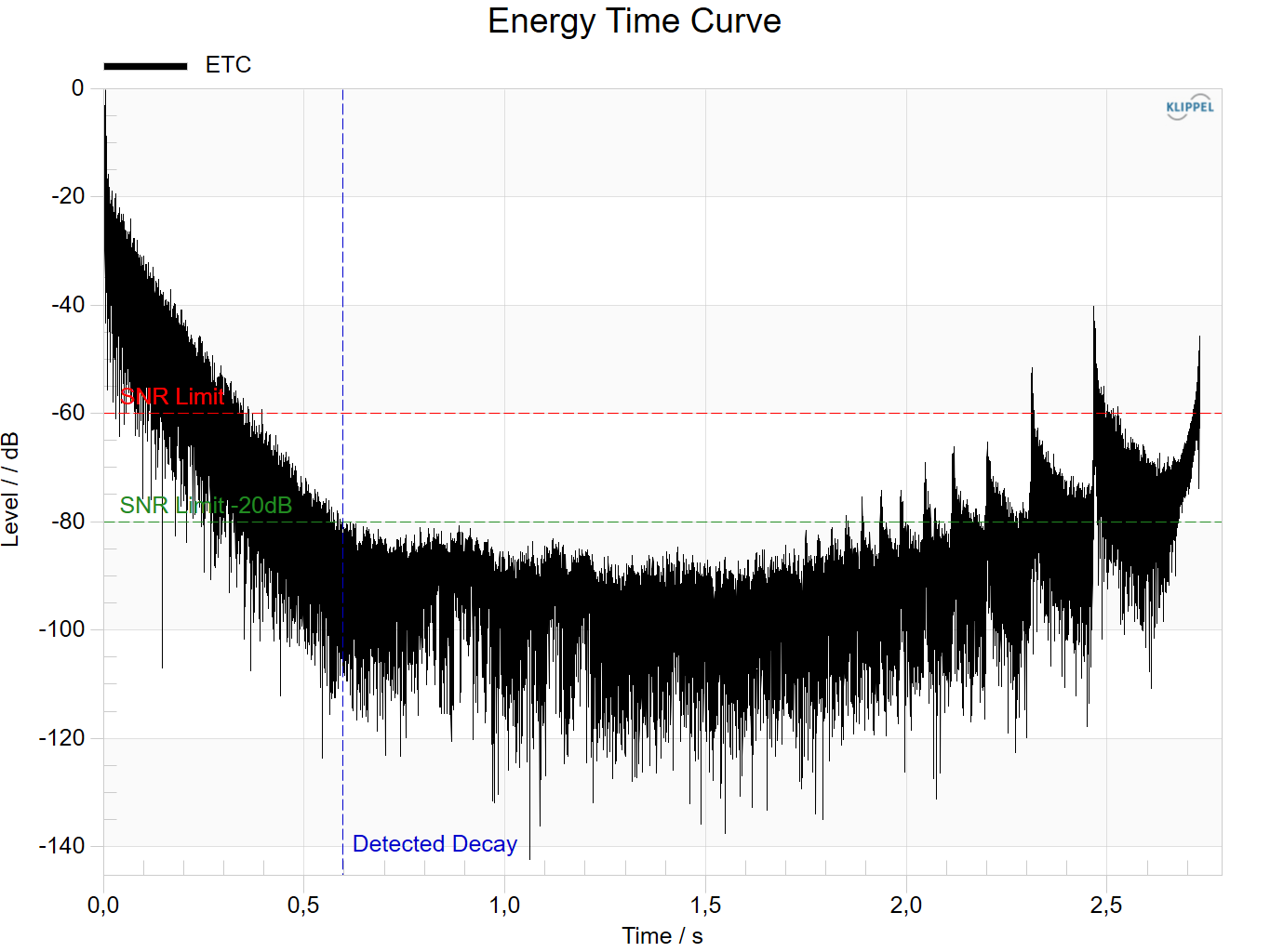
Energy Time Curve (ETC)

The Energy Time Curve (ETC) graph displays the energy decay of the impulse response. It provides a view of how the sound energy decreases over time in the measured room. The ETC is the analytical envelope of the impulse response of the In-Situ measurement, displayed on a logarithmic scale.

This curve is primarily used to perform additional checks to assess the quality of the In-Situ measurement:

• Measurement length: to verify that the recording was long enough to capture the full decay of the room.

• Signal-to-Noise Ratio (SNR): to confirm that the measurement has sufficient dynamic range for reliable analysis.

By reviewing the ETC, users can ensure that the measurement setup and recording conditions were appropriate before proceeding with further acoustic analysis.

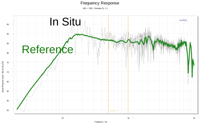
Frequency Response

The graph shows the frequency response of the In-Situ and Reference measurements, which are used to calculate the compensation filter.

Correction Curve

Transfer function of complex compensation filter. This filter can be used to correct the setup for further acoustic measurements. (e.g. TRF – Transfer Function Measurement, TBM – Tone Burst Measurement, etc.)

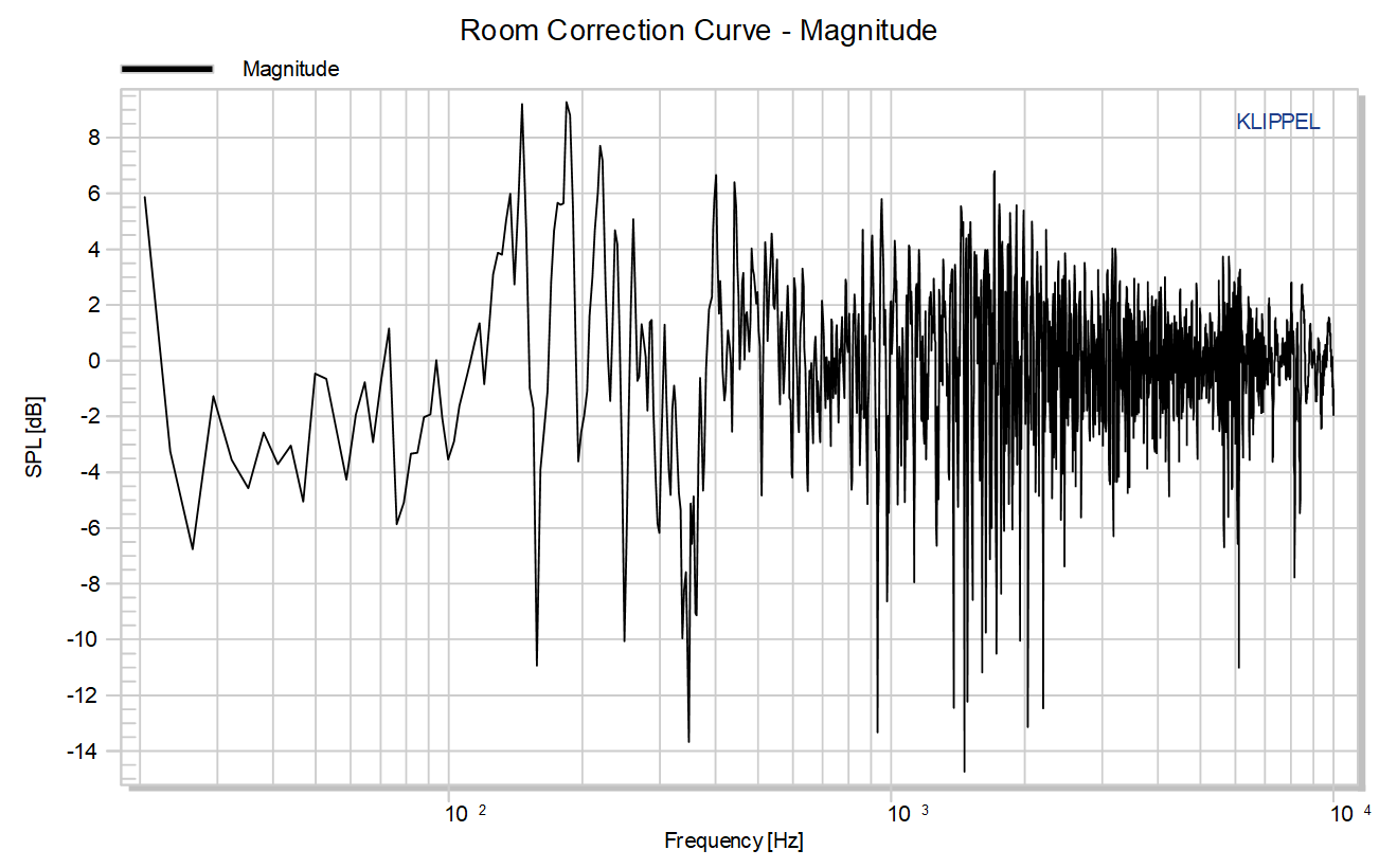
This filter is only valid for the current setup and needs to be recalculated when changing the Setup (e.g. changing position of speaker or microphone, measurement in a different room)

Supported Modules for Im/Export