SIM – Simulation

This module performs a numerical simulation of electro-dynamical drivers mounted in common enclosure systems. The following lumped-parameter model is used to describe the transfer behavior at low frequencies.

The inputs for the simulation routine are the parameters of a real or fictitious driver and enclosure system. For a one or two-tone excitation signal the response of electrical, mechanical and acoustical variables are calculated. A spectral analysis applied to the steady-state signals shows the amplitude and phase of the fundamentals and generated distortion components.

Simulations can be performed to investigate the voltage and/or frequency characteristic of distortion components and defined distortion measures. Analyzing these results in several states of the loudspeaker (pressure in front or behind cone, current, velocity, displacement etc.) allows a detailed investigation of the driver behavior and provides a high potential for optimizing the driver.

Note

This manual can be used for SIM (or SIM1) and SIM2 module. The SIM module is deprecated and replaced by SIM2. Results of SIM are displayed in current software version of dB-Lab, but no execution is allowed.

SIM - Tutorial

Overview

This module performs a numerical simulation of electro~dynamical drivers mounted in common enclosure systems. The following lumped-parameter model is used to describe the transfer behavior at low frequencies.

Overview

The inputs for the simulation routine are the parameters of a real or fictitious driver and enclosure system. For a one or two-tone excitation signal the response of electrical, mechanical and acoustical variables are calculated. A spectral analysis applied to the steady-state signals shows the amplitude and phase of the fundamentals and generated distortion components.

Simulations can be performed to investigate the voltage and/or frequency characteristic of distortion components and defined distortion measures. Analyzing these results in several states of the loudspeaker (pressure in front or behind cone, current, velocity, displacement etc.) allows a detailed investigation of the driver behavior and provides a high potential for optimizing the driver.

See also

E-Learning: Please also refer to the KLIPPEL e-learning online trainings for more information. Training 5 is dedicated to distortion prediction / simulation, including the SIM2.

What is the Goal of This Tutorial?

This tutorial makes you familiar with the SIM2 module.

The tutorial is divided into three parts.

1. In the first Viewing SIM Results (Part 1) we will show you how to view SIM results already stored in the web example database.

2. The next part of the tutorial Performing a new SIM (part 2) provides a step-by-step recipe to predict harmonic distortions in sound pressure, displacement, current, etc.

3. In the final section Customizing SIM (part 3) we discuss modifications of the setup parameters to use more powerful features and improve the performance of the module.

In the chapter SIM – Reference you will find more information about the nonlinear transducer model as well as a detailed description of the result windows and the configuration of the property pages.

Viewing SIM Results (Part 1)

Example data used in this manual is stored in the Web Example database. If not downloaded already, get it from the latest R&D release <https://www.klippel.de/go/current-rnd-release> and open the web-based database.

See also

View Results for general information on how to download this database, open and view results in dB-Lab.

Open Examples

Open and select the folder Simulation, Auralization (LSIM, SIM, SIM-AUR, DIF-AUR, ALS) / Simulation Auralization (SIM, SIM-AUR) / Simulation and open the object DIS-SIM comparison (DIS, SIM2, LSI). Please refer to the dB-Lab manual section for navigating within or selecting databases.

After double clicking on the operation 3b SIM SPL Harmonics the default result windows will be opened. First, we will have a look at the parameters of the used driver model. We assume an electro‑dynamic loudspeaker which can be modeled by an equivalent circuit. Open the property page Transducer. The numbers you see are the small signal (Thiele-Small) parameters of the driver. With these parameters the linear part of the driver is fully specified.

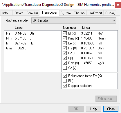
These are the most important parameters:

\(R_\text{e}\)

DC resistance of voice coil

\(L_{\text{e}}\)

frequency independent part of the voice coil inductance

\(Bl\)

force factor

\(K_{\text{ms}}\)

mechanical stiffness

\(f_\text{s}\)

driver resonance frequency

\(Q_{\text{ms}}\)

mechanical loss factor

For a detailed and complete explanation see section transducer property page in SIM Reference.

Nonlinerarities

The large signal curves of the driver are specified using the Edit curve … button.

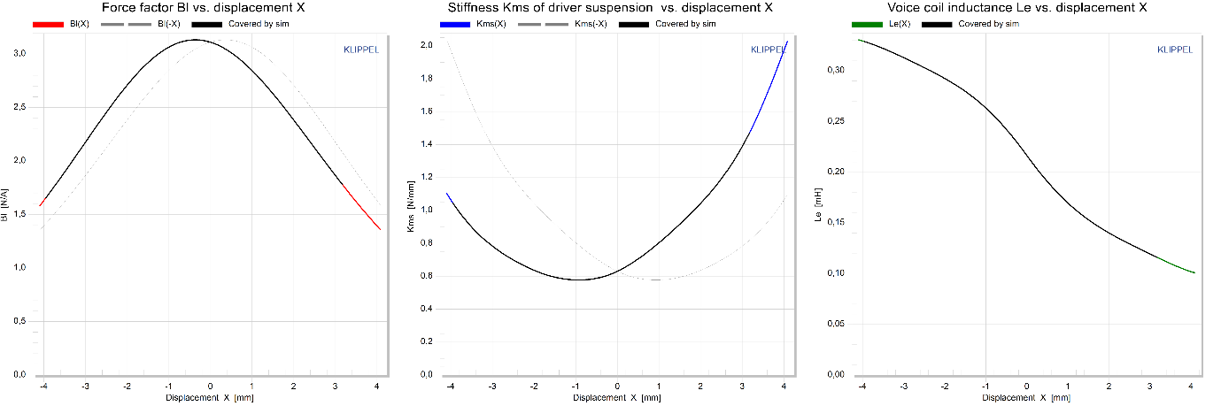
Open parameters the Bl(X) and Kms(X) result windows. In the large signal domain, the force factor \(Bl\) and the suspension stiffness \(K_{\text{ms}}\) are displacement dependent. If the adjacent checkboxes are selected the displacement dependent characteristics will be used instead of the constant characteristics \(Bl(x) = \text{const.}\) and \(K_{\text{ms}}(x) = \text{const.}\) In this example the nonlinear dependency of Bl, L_e, K_ms, L₂ and R₂ on the displacement x was incorporated into the simulation model as well as the reluctance force F_m(x) and the Doppler effect. This data was imported from the Large Signal Identification (LSI or LSI3) measurement.

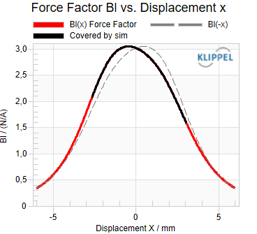
Force Factor \(Bl\) vs. Displacement x

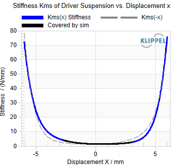
Stiffness \(K_{\text{ms}}\) of Driver Suspension vs. Displacement x

System properties

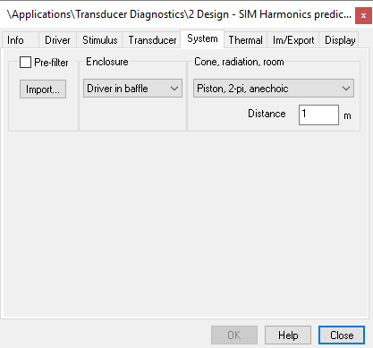
In the property page System, you can select the particular driver enclosure for which the simulation shall be performed. In this example a driver mounted in a baffle was chosen. No pre‑filter was used. The sound pressure in the far field was calculated using a simple 2π radiation model for a distance of 1 meter.

Now open property page Thermal. This page is for specifying the thermal model.

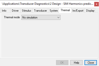
In our example the simplest thermal model was used. The voice coil was assumed to be always at ambient temperature (no thermal simulation). This is valid if the driver is heated only slightly during operation.

Stimulus

Now the last measurement Setup page specifying the excitation is analyzed. Open the property page

Stimulus.

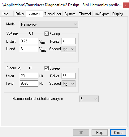
Identical to the DIS – Distortion module, several excitation modes can be selected. Here a Harmonic Analysis has been chosen. The simulation was performed sequentially for different voltages. The frequency was stepped from 20 Hz to 9560 Hz (98 points spaced logarithmically).

Results

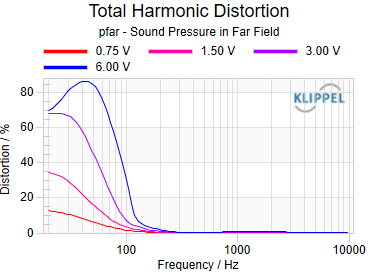
One of the default windows which are opened at double clicking the operation name is THD Total Harmonic Distortion. The result window shows the total harmonic distortion of the SPL signal in 1m distance on axis as specified above versus excitation frequency f₁.

THD vs. level and frequency

Open now the property page Display and select 3D Plot. The Fundamental result window will now be shown as a surface plot vs. voltage and frequency. You can clearly recognize the variation of SPL versus frequency and voltage. Switch back to 2D versus frequency.

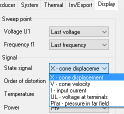
Set on the Display property page the State signal to X ‑ cone displacement.

Now the fundamental of the displacement signal is shown. You may also switch to all other available states in this selection box. This allows you to perform a powerful analysis of the mechanisms within the simulated driver even at positions, where you can’t measure.

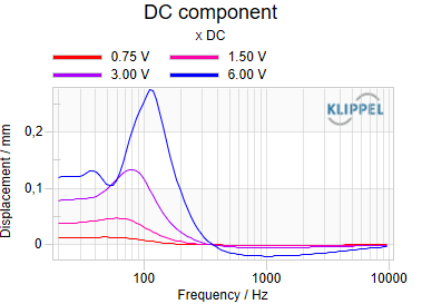
Open the result window DC Component from the result window list. Here the dynamically generated DC component of the driver is shown. Depending on frequency and level, the AC part of the excursion due to the (pure) AC excitation is superimposed by a DC part. This DC part is generated by the nonlinear characteristics of the driver. In this example the stiffness is not symmetrical. This shifts the momentary rest position to negative displacements (towards the magnet structure of the driver, moves “in”).

DC component vs. level and frequency

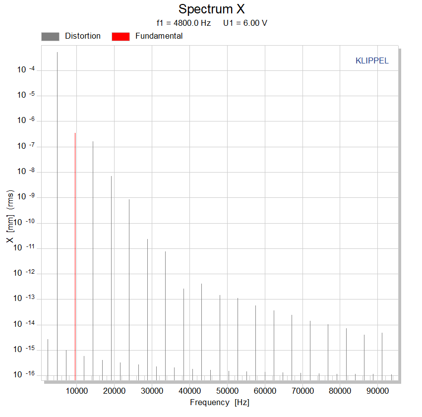
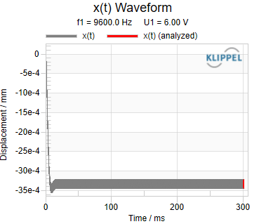
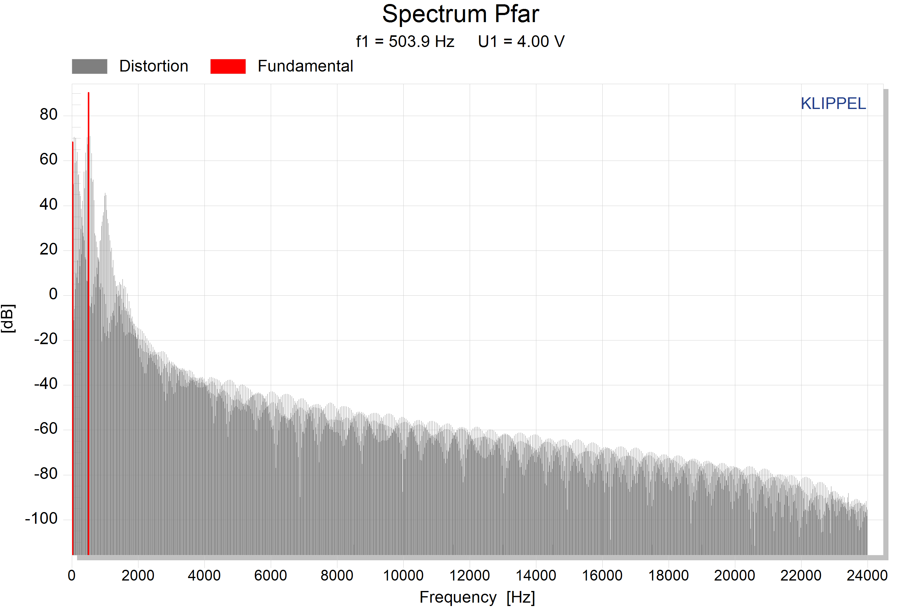
Open the result windows Spectrum and Waveform and look at the spectral components and the time signal of the displacement signal. In order not to inflate the database size the spectra and waveforms are stored only for the last simulated sweep point (rather than for all sweep points). The spectrum and time signal you look at is therefore the data for maximum level and highest frequency. Since the displacement and therefore the harmonic distortion is low for higher frequencies, the time signal looks very sinusoidal. However, in the spectra clearly the harmonic components are visible.

Comparison with DIS Measurement

As noted before, the SIM module is designed to be comparable to the DIS measurement module. The setup data and result windows are very similar or identical. You may compare the simulation with the measurement at the end of this first tutorial part. Open the window THD Total Harmonics Distortion of the operations 3a DIS SPL Harmonics and 3b SIM SPL Harmonics. The identical setups for SIM and DIS allow a comparison of both results. Please set the “Display” settings to Pfar - pressure in Far Field (SIM2) and Signal at IN1 (DIS).

DIS Measurement of THD

SIM2 Simulation of THD

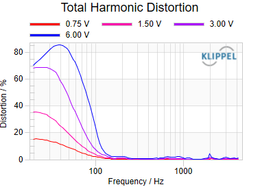
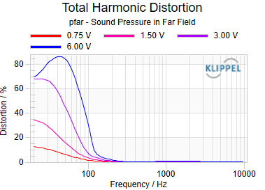
You may also perform comparisons on the fundamental and the DC component of the displacement x. There is an Application Note available on how to perform comparable operations with SIM and DIS “AN17 Credibility of Nonlinear Parameters”.

Note

The magnitudes given in all spectral representations are rms magnitudes (i.e. \(\text{peak magnitude} / \sqrt{2}\) ). For consistency reasons, displacements are given in mm (rms). The corresponding peak displacement is calculated by multiplying the given displacement by\(\ \sqrt{2}\). An exception is the DC component where the rms value is equal to peak. Especially for comparing the DC component with the fundamental (which is given in rms) care must be taken to consider the additional factor.

Performing a new SIM (part 2)

In the second part of the tutorial a step~by~step recipe is provided to simulate a driver in order to predict harmonic distortion of the sound pressure and displacement. The SIM2 module needs the parameters of a real or conceptional driver. In the tutorial we are going to simulate one of your own drivers for which you have already determined the large signal parameters via Large Signal Identification (LSI or LSI3).

Note

The nonlinear parameters can be conveniently transferred from the LSI or LSI3 module to the SIM2 module. For this, the parameters are exported from LSI or LSI3 to clipboard and imported from clipboard into SIM.

Connect the Hardware

1. Connect a Klippel, Dongle, KA3 or DA with the computer via USB.

2. Klippel Analyzer 3 (KA3) or Distortion Analyzer (DA): Connect power supply to measurement device.

Select Setup Parameter

1. Open database which includes an already performed Large Signal Identification using the LSI or LSI3 module.

2. Click at the driver and create a new SIM operation.

3. Open the LSI operation and press Export to clipboard in property page Im/Export in order to copy the large signal driver parameters to the clipboard.

4. Open the new SIM operation and press Import from clipboard in property page Im/Export to import the parameters from the clipboard.

5. Open property page Stimulus. In this page you have to specify the excitation signal. Select Voltage: Sweep. Use the default setting for voltage and frequency sweep.

6. As we are not going to predict intermodulation distortion set Mode to Harmonics. That way the second excitation tone is switched off and the simulation is speeded up.

7. Open property page System and select Driver in baffle.

8. Open property page Transducer and select the LR-2 inductance model. If not checked, activate the checkboxes

   • Bl(x),

   • Kms(x),

   • Le(x), L2(x), R2(x),

   • Reluctance Force Fm(x), and

   • Doppler radiation.

9. Open property page Thermal and select No simulation as thermal mode.

Start Simulation

1. Start measurement by pressing the button Run .

2. You may pause the simulation by pressing Pause .

3. The measurement will be canceled if you press Cancel .

Wait until the simulation has finished.

View Results

1. Open result windows by setting the checkbox in the list of results.

2. Open property page Display. Set State signal to Pfar – pressure in far field in order to show the distortion of the sound pressure.

3. Set State signal to X – cone displacement and look at the distortion of the displacement.

4. The result windows Waveform and Spectrum show waveforms and spectra for the last sweep point. In order to keep the size of the database reasonably small the waveform and spectra for the other sweep points are not stored. However, you might want to look at some waveform or spectrum for a particular sweep point that are not stored. You can get this information by repeating the simulation just for the single sweep point of interest.

5. Press the button Run . You will see a message box.

   Click at Single point measurement and select the voltage and frequency of the sweep point you are interested in. Confirm with OK. After the single point simulation has finished the time signal and spectra are shown for the selected voltage-frequency point.

Note

In case of very high excitation levels the displacement x may exceed the range for which the nonlinear parameters are defined/measured for. The large signal parameters can differ widely from physics outside the defined/measured range. In case the displacement exceeds the defined range Xpse you will get a warning. Cancel the sweep and increase Xpse in the curve edit dialog that can be opened by pressing the button Edit curve … in property page Transducer. Check the results windows Bl(x), Kms(x) and Le(x) which show the nonlinear parameters for the new Xpse range. If the parameters are still reasonable you can start the simulation again. If not, decrease the excitation level.

Customizing SIM (part 3)

In this part of the tutorial, we discuss modifications of the setup parameters to use more powerful features and to improve the performance of the module.

How to Generate Your Own Nonlinear Parameters

The SIM module provides a curve editor to modify the shape of the nonlinear parameters or generate the parameters of a fictional driver. This is useful to investigate design choices. There are two possibilities. Either you start with the parameters of a measured driver and modify the power series coefficients or you generate the nonlinearities from scratch. If you generate the parameters from scratch you can either start from a constant curve or import an external curve. If an external curve is imported the according power series coefficients will be calculated to fit the imported curve shape.

To synthesize nonlinear parameters, open property page Transducer or System. Select the nonlinearity you want to generate and click the Edit curve… button. You will see a dialog with three different pages. The (x-axis) range over which the nonlinear curve is defined can be specified in the top left corner of all three pages (pse = range of power series expansion).

In the Regular page you can specify and modify the coefficients of the common (regular) power series. The order of the power series can be modified with the Order drop down box.

Edit Bl(x) non-linearity curve as regular series expansion

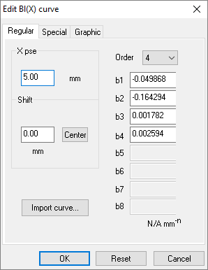
The Special page gives access to the coefficients the special power series. In contrast to the regular power series this series is more suited to the driver physics. Regardless what coefficients you choose it will never be negative. See section sim2-reference | Property pages | How to edit the nonlinear parameters for exact equations and further information. The order of the power series can be modified with the Order drop down box.

The Graphic page provides five sliders for modifying the curve shape graphically.

Edit Bl(x) curve in graphic manipulation mode

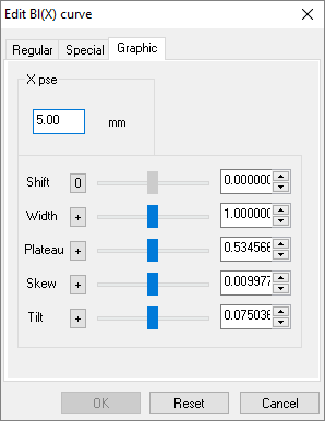
• Shift controls the horizontal shift of curve. It can be used to center the nonlinearity by shifting the curve maximum to x =0.

• Width is the width of the curve. The curve can be made wider or narrower. Use the slider to adjust the point at which the force factor drops to 50 percent. This corresponds to the (half) gap width (underhang configuration) / voice coil height (overhang configuration).

• Plateau controls the region around the rest position. The slider changes its shape from plateau like to peak like.

• Skew controls the asymmetry of the curve. The curve can be made more symmetric/skewed referred to the zero-axis.

• Tilt controls the overall slope of the curve. The slope contributes to the asymmetry and can be positive or negative.

To change the slider range drag the slider to the boundary and hold it. Holding the slider at the right (left) boundary will shift the range upwards (downwards). The shift can be accelerated by pressing the SHIFT button simultaneously. The button left of the slider is for changing the sign of the curve parameter. Pressing the button will toggle the sign between positive, negative and zero. If zero is selected the parameter value is set to zero. Alternatively edit boxes right of the sliders can be used to enter the curve parameters directly.

To generate a curve from scratch specify adjust first the Width slider. Than use the Plateau and Shift slider to specify the curve plateau and offset. Finally adjust the curve asymmetry with the Skew and Tilt sliders.

While adjusting curve shapes it is sometimes useful to compare with the original curve. In order to view the original curve, open the curve editor and right click at the result window. Choose Customization Dialog…| Subsets and select the Original subset.

An external curve can be imported by clicking at the Import curve… button in pages Regular and Special. This opens a dialog where a curve can be imported from the clipboard in order to calculate the corresponding power series coefficients. For this the curve must be represented as two-column matrix where the first column gives the x-values and the second the y-values. See section Curve Im/Export later in the Reference for more information about the import format.

An existing curve can be shifted horizontally by clicking the Set button in the group Shift in pages Regular and Special. This is for instance useful to center the force factor or compliance curve by shifting the curve maximum to x =0. The default shift value will move the curve maximum to x =0. New power series coefficients will be calculated to fit the shifted curve. The Shift operation can be performed repeatedly.

How to View Waveforms and Spectra?

In order not to inflate database size the complete waveform and the according spectra of each sample point are not stored in the database. However, inspecting the waveform or the spectra is often quite useful. During the simulation waveform and spectra can be viewed for the most recent sweep point. If you pause the simulation by pressing Pause, waveform and spectra for the current sweep point. After the simulation has finished the above result windows will show the waveform and spectra for the last sweep point. If you want to view waveform and spectra for a particular sweep point you can repeat the simulation for this single sweep point. Press Run. A message box will pop up. Click at Single point measurement and select the voltage and frequency of the sweep point you are interested in. Confirm with OK. After the simulation has finished waveform and spectra are shown for the selected sweep point.

How to Copy the Stimulus Settings from or to a DIS

The SIM and the DIS modules are ‘twins’. Many result windows and setup parameters correspond to each other. A common application is to simulate a speaker and to compare the simulation results to the results measured with DIS. The same voltage-frequency sweep should be used for this. The Stimulus settings of SIM can easily be copied to DIS:

1. Open property page Im/Export of SIM and press Export to clipboard .

2. Open property page Im/Export of DIS and press Import from clipboard .

To copy the setting from DIS to SIM press first the Export button in DIS and then the Import button in SIM .

Speed up simulation

There are several ways to speed up the simulation:

1. If you want to predict only harmonic distortion and no intermodulation distortion, use the Harmonics Mode in the property page Stimulus. A simultaneous measurement of harmonic and intermodulation distortion will take considerably more time than a sole harmonic measurement.

2. In property page Im/Export you can select the solver used for numerical simulation. If you select Fast simulation, a numerical solver without step size control will be used to calculate the nonlinear model equations. This solver is very fast and will calculate in most cases the exact speaker states. In some few cases the precision will suffer and a more sophisticated solver with step size control has to be used. If that is the case, an error will appear. Please change then the solver to Precise simulation.

Linear / dB Y‑Axis of Result Windows

The user can adjust the spacing of the y-axis for the result windows

• Fundamental

• Harmonic (n)

• Diff. Intermod (n)

• Sum. Intermod (n) and

• Peak + Bottom.

in property page Display.

First, linear (Lin) or logarithmic (Log) spacing can be chosen. If Auto is selected the representation of the y-axis values depends on the spacing of the voltage sweep selected in property page Stimulus (Voltage U1: Spaced). For a linear voltage sweep the y-axis values will be spaced linearly whereas for a logarithmic voltage sweep the y-axis values will be given in dB. This way amplitude compression effects can be visualized if 2D and versus f1 is selected in property page Display . In case of no amplitude compression the curves for different sweep voltages are equidistant. Any compression will alter the distance between the curves. The y-axis spacing (Lin /Log /Auto ) can be selected independently for the individual speaker states signals.

Add Comments

The Info property page allows the user to change the name of the operation and to add a comment to the measurement (comments may be included in the report file).

SIM – Reference

Overview

This module performs a numerical simulation of electro-dynamical drivers mounted in common enclosure systems. An extended lumped-parameter model is used to describe the transfer behavior in the full working range. The input of this routine are the parameters of a real or fictitious driver and enclosure system. The dominant nonlinearities of the driver (motor and suspension), the enclosure (air compression, flow resistance of the vent, stiffness of passive radiator) and radiation (Doppler-Effect) are considered. The thermal behavior of the driver is simulated using nonlinear thermal model that considers air convection cooling. For a two-tone excitation signal the responses of electrical, mechanical and acoustical variables are calculated. A spectral analysis applied to the steady-state signals shows the amplitude of the fundamentals, the DC component, generated distortion components and the temperature of the voice coil, the gap and the magnet.

A series of simulations can be performed to investigate the voltage and/or frequency characteristic of distortion components and distortion measures.

Each nonlinearity in the system can be switched off to investigate its effect systematically. Thus this module shows the dominant sources of distortion and gives valuable indications for driver optimization. An editor supports the modification of the driver nonlinearities to simulate new ideas in the initial development stage.

Theory

Transducer Modeling

At first, we provide a short overview on the large signal modeling of electro-dynamical drivers mounted in enclosures which considers the dominant driver nonlinearities and the nonlinear thermal mechanisms like air convection cooling.

State Variables

The state of a speaker operated at low frequencies where the wavelength is large in comparison to the geometrical dimension can be described by using the following quantities:

\(x(t)\)

displacement of the voice coil \(x(t)\)

\(v(t)\)

velocity of the voice coil

\(i(t)\)

the electric input current

\(u(t)\)

the driving voltage at loudspeaker terminals

\(p_{\text{box}}(t)\)

sound pressure in enclosure (AC-part)

\(q_{\text{P}}(t)\)

volume velocity in port

\(x_{\text{r}}(t)\)

displacement of passive radiator

\(p_{\text{rear}}(t)\)

sound pressure in rear enclosure

\(p_{\text{far}}(t)\)

sound pressure in the far field

Lumped Parameter Model

The relationship between the state variables can be described by a lumped parameter model comprising a few elements characterized by parameter values. The number and kind of the lumped elements and the way how they are connected is called the topology of our model. It is graphically represented as an electrical equivalent circuit. The speaker is considered as a transducer coupling the electrical, mechanical and acoustical domain. In contrast to the traditional linear modeling some parameters are not constant but depend on displacement, current, voice coil temperature, etc…

Lumped Parameter Model

Electrical Driver Parameters

The electrical part comprises the following elements:

\(R_{\text{e}} (T_{\text{v}})\)

DC resistance of voice coil

\(L_{\text{e}} (x,i)\)

part of voice coil inductance which is independent on frequency comprising a displacement and current varying part \(L_{\text{e}}(x,i)=L_{\text{e}}(x,i=0)\cdot\frac{L_{\text{e}}(x=0,i)}{L_{\text{e}}(x=0,i=0)}\)

\({L_2(x,i_2), L_3(x,i_2)}\)

represents the para-inductance of the voice coil comprising a displacement and current varying part

\[L_2(x,i_2)=L_2(x,i_2=0)\cdot \frac{L_2(x=0,i_2)}{L_2(x=0,i_2=0)}\]

\[L_3(x,i_3)=L_3(x,i_3=0)\cdot \frac{L_3(x=0,i_3)}{L_3(x=0,i_3=0)}\]

\({R_2(x,i), R_3(x,i)}\)

the electric resistance due to additional losses caused by eddy currents

Mechanical Driver Parameters

A transformer with the coupling factor

\[Bl(x,i)=Bl(x)\cdot [1+F(x)\cdot i]\]

connects the electrical with the mechanical domain where

\(Bl(x)\)

is the effective instantaneous electro-dynamic coupling factor (force factor of the motor) defined by the integral of the permanent magnetic flux density \(B\) over voice coil length \(l\)

\(F(x)\)

is effective flux modulation caused by alternating magnetic field generated by the voice coil current

The variation of the magnetic field energy versus voice coil displacement generates a reluctance force \(F_{\text{m}}(x, i, i_2, i_3)\) which can be approximated by

\[F_{\text{m}}(x,i,i_2,i_3)\approx-\frac{i(t)^2}{2} \frac{∂L_{\text{e}}(x)}{∂x}- \frac{i_2(t)^2}{2}\frac{∂L_2(x)}{∂x}-\frac{i_3(t)^2}{2}\frac{∂L_3(x)}{∂x}\]

The mechanical system is represented by the following elements

\(M_{\text{ms}}\)

mechanical mass of driver diaphragm assembly including voice-coil and air load

\(R_{\text{ms}}(v)\)

Nonlinear mechanical resistance versus voice coil velocity v representing driver suspension losses, air turbulences, air radiation load

\(K_{\text{ms}}(x)\)

mechanical stiffness of driver suspension

Acoustical Parameters

The area of the diaphragm connects the mechanical and acoustical domain:

\(S_{\text{d}}\)

effective projected surface area of driver diaphragm

The driver enclosures (band-pass, sealed, vented, passive radiator) may be modeled by using the following elements:

\(R_{\text{al}}\)

acoustic resistance of enclosure losses caused by leakage

\(M_{\text{ap}}\)

acoustic mass of port or vent including air load

\(R_{\text{ap}} (q_{\text{p}})\)

acoustic resistance of port or vent losses

\(K_{\text{mr}} (x_{\text{r}})\)

mechanical stiffness of passive radiator

\(K_{\text{ab}} (p_{\text{box}})\)

acoustic stiffness of air in enclosure

\(K_{\text{r}} (p_{\text{rear}})\)

acoustic stiffness of air in rear enclosure in band-pass systems

\(V_{\text{r}}\)

volume of air in rear enclosure in band-pass systems

\(v_{\text{b}}\)

volume of air in enclosure

where

\[K_{\text{ab}}(p_{\text{box}})=\frac{1}{\frac{V_{\text{ab}}}{\gamma p_0}\cdot \left[ 1-\frac{\gamma+1}{2\gamma}(\frac{p_{\text{box}}}{p_0})+\frac{\gamma+1}{6\gamma}(2+\frac{1}{\gamma}) (\frac{p_{\text{box}}}{p_0})^2 \right] }\]

\[K_{\text{r}}(p_{\text{rear}})=\frac{1}{\frac{V_{\text{r}}}{\gamma p_0} \cdot\left[ 1-\frac{\gamma+1}{2\gamma}(\frac{p_{\text{rear}}}{p_0})+\frac{\gamma+1}{6\gamma}(2+\frac{1}{\gamma}) (\frac{p_{\text{rear}}}{p_0})^2 \right] }\]

γ is the adiabatic coefficient (γ= 1.4) and \(p_o= 101,3 \text{kN}/\text{m}^2\) is the static air pressure.

Thermal Modeling

The heating of the voice coil is modeled by a nonlinear thermal equivalent circuit

Thermal Model of an electro-dynamic Transducer

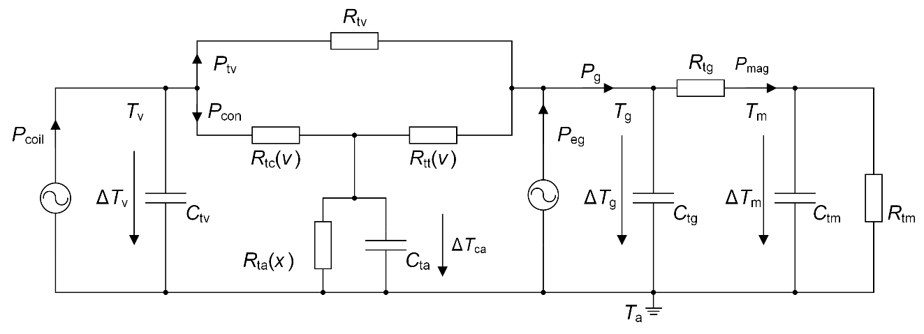
comprising the following elements and state variables:

\(R_{\text{tv}}\)

thermal resistance of path from coil to pole tips and magnet surface

\(R_{\text{tm}}\)

thermal resistance of path from magnet to ambient air

\(R_{\text{tg}}\)

thermal resistance of path from pole tips to magnet and frame

\(C_{\text{tv}}\)

thermal capacitance of voice coil and voice coil former (not used for simulation)

\(C_{\text{tm}}\)

thermal capacitance of magnet and frame (not used for simulation)

\(C_{\text{tg}}\)

thermal capacitance of pole tips and magnet surface close to coil (not used for simulation)

\(R_{\text{tc}}(v)\)

thermal resistance of path from coil to air in the gap due to convection cooling

\(R_{\text{ta}}(x)\)

thermal resistance of path from air in the gap to ambience due to convection cooling

\(R_{\text{tt}}(v)\)

thermal resistance of path from air in the gap to the magnet structure due to convection cooling

\(p_{\text{coil}}\)

power dissipated in voice coil and former

\(p_{\text{eg}}\)

power transferred to the pole tips due to eddy currents

\(p_{\text{g}}\)

power transferred to the pole tips

\(p_{\text{tv}}\)

power transferred to the pole tips from coil

\(p_{con}\)

power transferred to the air in the gap due to convection cooling

\(\gamma\)

bypass factor

\(T_{\text{v}}\)

temperature of the voice coil

\(T_{\text{m}}\)

temperature of the magnet structure

\(T_{\text{g}}\)

temperature of the pole tip

\(T_{\text{a}}\)

temperature of the cold transducer (ambient temperature)

\(\Delta T_{\text{v}} =T_{\text{v}}-T_{\text{a}}\)

increase of voice coil temperature

\(\Delta T_{\text{g}} =T_{\text{g}}-T_{\text{a}}\)

increase of temperature of the pole tips

\(\Delta T_{\text{m}} =T_{\text{m}}-T_{\text{a}}\)

increase of the temperature of magnet structure

The nonlinear thermal resistances,

\[R_{\text{ta}} (x)=\frac{1}{x_{\text{rms}}\cdot r_{\text{x}}}\]

\[R_{\text{tc}}(v)=\frac{1}{v_{\text{rms}}\cdot r_{\text{v}}}\]

\[R_{\text{tt}}(x)=\frac{1}{x_{\text{rms}}\cdot r_{\text{b}}}\]

the powers

\[P_{\text{eddy}}=R_2\cdot (i-i_2)^2+R_3\cdot (i-i_3)^2\]

\[P_{R_{\text{e}}}=R_{\text{e}}\cdot i^2\]

\[P_{\text{coil}}=P_{R_{\text{e}}}+\alpha\cdot P{\text{eddy}}\]

\[P_{\text{eg}}=(1-\alpha)\cdot P_{\text{eddy}}\]

and the bypass factor

\[\gamma=\frac{P_{\text{con}}+P_{\text{eg}}}{P_{R_{\text{e}}}+P_{\text{eddy}}}\]

are described by the following parameters:

\(r_{\text{x}}\)

convection cooling parameter considering the effect of cone displacement

\(r_{\text{v}}\)

convection cooling parameter describing the dependence of \(R_{\text{tc}}\) from cone velocity

\(r_{\text{b}}\)

convection cooling parameter describing the dependence of \(R_{\text{tt}}\) from cone velocity

\(\alpha\)

factor describing the distribution of heat caused by eddy currents on voice coil and magnet

Thermal simulation modes

Three different simulation modes are supported. All simulate steady state thermal conditions.

1. Short term. This mode simulates the short-term thermal behavior. It is assumed that the voice coil temperature has reached steady-state while the magnet is still cold \((\Delta T_{\text{m}}=\Delta T_{\text{g}}=0)\) . This means that the thermal capacitances \(C_{\text{tg}},C_{\text{tm}}\) are shorted and \(C_{\text{tv}}\) has infinite resistance.

2. Long term. This mode simulates the long-term thermal behavior. Both voice coil and magnet temperature are assumed to be hot and in steady-state. In this state all thermal capacitances of the model have infinite resistance.

3. No simulation. The thermal simulation is switched off. Voice coil and magnet are assumed to be at ambient temperature.

The user can simplify the model by switching off the thermal resistances \(R_{\text{ta}}(x),R_{\text{tc}}(v),R_{\text{tt}}(v),R_{\text{tg}}\) and the direct heating due to eddy currents (\(\alpha\)). This is useful if the corresponding thermal parameters are unknown.

Interaction between thermal and electro-mechanical model

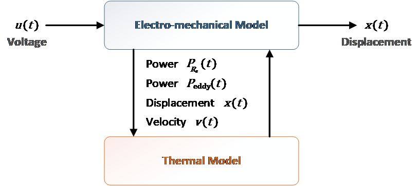
The thermal model is coupled to the electro=mechanical model by the state variables \(x,v,i,i_2,i_3\) and the voice coil temperature \(T_{\text{v}}\) . The electro-mechanical model supplies the displacement \(x\) , the velocity v and the powers \(P_{R_{\text{e}}}=R_{\text{e}}\cdot i^2\) and \(P_{\text{eddy}}=R_2\cdot (i-i_2)^2+R_3\cdot (i-i_3)^2\) to the thermal model while the temperature increase \(\Delta T_{\text{v}}\) is given back to the resistance \(R_{\text{e}}\).

Coupling of thermal and electro-mechanical Model

State Space Equation

We assume that all effects of the acoustical environment and the radiation impedance may be represented by the acoustical and mechanical parameters which are independent on the radiated sound pressure \(p_{\text{far}}\) .

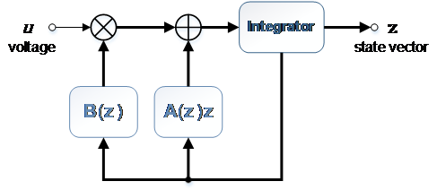
Thus, the differential equation written in the general state space form is

\[\dot {\textbf{z}} = \textbf{a(z)} \cdot \textbf{z} + \textbf{b(z)} \cdot u\]

where \(u\) is the voltage at the terminals of the voltage driven loudspeaker,

\[\textbf{z}(t)=\left[ x\frac{dx}{dt}i\ i_2\ i_3\ p_{\text{box}}\ q_{\text{p}}\ x_{\text{p}}\ p_{\text{rear}} \right]^T\]

is the state vector of the system, and the matrix \(\textbf{z}\) and the vector \(\textbf{b}\) comprise lumped parameters depending on the state vector \(\textbf{z}\).

The graphical representation of the state space form reveals a feed-back structure where all the distorted signals in the state vector \(\textbf{z}\) react via the nonlinear parameters on the input of the system.

Pre-filter

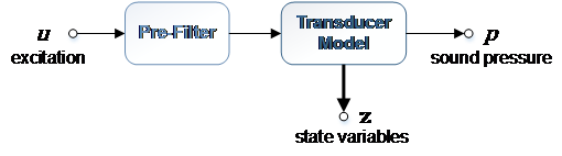
The excitation voltage \(u(t)\) may be modified by pre=filter. This is useful to include crossovers into the simulation. The frequency response \(H_{\text{pre}}(f)\) (magnitude and phase vs. frequency) of the filter can be imported from the clipboard. If the filter phase response is not available, it is sufficient to import the magnitude response only. In this case the phase of the excitation signal will be left unchanged. The transducer model including pre-filter is shown underneath.

Cone, Radiation, Room

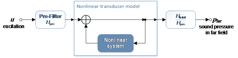
Two different ways to calculate the sound pressure in the far field are supported. The first one is to use a simple model that assumes a piston like cone and “ideal” 2π-or 4π-radiation without any deterioration of the rooms. The second option is to import the total frequency response \(H_{\text{total}}=P_{\text{far}}(f)/U(f)\) which may either be measured or synthesized.

Simple model

The sound pressure signal in the far field is approximated by

Driver in Baffle:

\[p_{\text{far,simple}}(t)=\alpha\cdot S_{\text{d}}\cdot \frac{dv}{dt}\]

Closed Box, Vented Box, Passive Radiator:

\[p_{\text{far,simple}}(t)=-\alpha\frac{d^2(C_{\text{ab}}(p_{\text{box}})\cdot p_{\text{box}})}{dt^2}\]

Bandpass:

\[p_{\text{far,simple}}(t)=\alpha\frac{dq_{\text{p}}}{dt}\]

where the factor α is \(\frac{p}{2\pi r}\) for the 2π - radiation and \(\frac{p}{4\pi r}\) for the 4π-radiation and

\(p\)

density of air,

\(c\)

speed of sound,

\(r\)

distance between diaphragm and listening position.

Import of total frequency response

Instead of some model for the cone, radiation and room the total transfer function \(H_{\text{total}}(f)=P_{\text{far}}(f)/U(f)\) can be imported. Rooms of small and medium size effect the far field sound pressure signal. The transmission varies considerably with frequency and listening position and the relationship between frequency and transmission is usually very complicated. However, this relationship can easily be measured for instance with the TRF module of the Klippel R&D System. Using a measured transfer function \(H_{\text{total}}(f)\) leads to simulation results that consider the influence of the cone breakup modes, the radiation and the room reflections. This way the sound pressure for the actual listening environments can be simulated and easily compared with the measured sound pressure. The calculation of the sound pressure in far field using an imported total frequency response \(H_{\text{total}}(f)\).

Large Signal Parameters

Dominant Large Signal Parameters

The linear, nonlinear and thermal parameters of the driver can be identified with the LSI – Large Signal Identification module which is part of the Klippel R&D System. The LSI module provides the coefficients of the corresponding power series expansions. All of the driver parameters may be copied to the clipboard and imported to SIM. The type and the parameters of the enclosure and radiation conditions may be specified. No import parameters are required to consider the nonlinear compliance of the air in the enclosure and nonlinear radiation due to the Doppler effect. This module also provides a nonlinearity editor to modify the shape of the nonlinearities and to investigate the performance of design choices.

Simulation Technique

Signal Generation

A two-tone signal defined by

\[u(t)=U_1\cdot sin(2\pi\cdot f_1\cdot t)+U_2\cdot sin(2\pi\cdot f_2\cdot t)\]

is an optimal excitation signal to measure harmonic, difference-tone and summed-tone intermodulation components. The frequencies \(f_1\) and \(f_2\) and the voltage \(U_1\) and \(U_2\) may be specified by the user. They may be varied automatically to perform frequency and voltage sweeps.

Frequency Sweep

The user can choose between a single point measurement performed with constant and a series of sequential measurements performed for different values of \(f_1\) . The user has to specify the start value \(f_{\text{start}}\) and the end value \(f_{\text{end}}\) for the frequency \(f_1\) as well as the number of intermediate points spaced linearly or logarithmically.

Voltage Sweep

The user can choose between a single point measurement performed with constant and a series of sequential measurements performed for different values of \(U_1\) . The user has to specify the start value \(U_{\text{start}}\) and the end value \(U_{\text{end}}\) for the Voltage \(U_1\) as well as the number of intermediate points spaced linearly or logarithmically. The voltage \(U_2\) of the second tone is coupled to the voltage \(U_1\) of the first tone and the user specifies the ratio \(U_2/U_1\).

Measurement of Harmonics

The user can choose between the different measurement modes. The Harmonics mode is used to measure the harmonic components of tone \(f_1\). The second excitation tone is switched off. This reduces the amplitude of the excitation signal \(u(t)\) and avoids interference between harmonic and intermodulation components.

Measurement of Intermodulations

In the Harmonics + Intermodulation (f1) and Harmonics + Intermodulations (f2) modes summed-tone and difference-tone intermodulation components (centered around \(f_1\) and \(f_2\) respectively) are measured additionally to the harmonic components of \(f_1\). No harmonic components are measured if Intermodulations(f1) is selected.

There are three different modes to specify the frequency \(f_2\) of the second tone:

• The frequency \(f_2\) is held constant during frequency sweep of \(f_1\). This mode allows to generate very critical stimuli for most transducers. Selecting \(f_2\lt f_1,f_2\) may represent a bass tone producing large voice coil displacement and \(f_1\) represents any audio component (voice) in the pass band of the transducer.

• The distance \(f_2-f_1\) between both excitation frequencies is constant during the frequency sweep of \(f_1\). This mode produces difference intermodulation at the same frequency independent of \(f_1\).

• The frequency ratio \(f_2/f_1\) is held constant between both excitation tones. Selecting \(f_2\gt f_1\) and using a fractional ratio (e.g. 5.5) this mode avoids interference between the harmonic and intermodulation distortion components.

Sample Rate

The excitation signal is sampled at 48 kHz to simulate the transducer up to 24 kHz signal components. Internal oversampling is used to simulate higher order frequency components (harmonic and intermodulation distortion), as well as to minimize simulation errors.

Solving the Differential Equation

The numerical integration may be accomplished by the classical explicit RUNGE-KUTTA method or by more sophisticated solvers with step size control giving higher precision. For certain combinations of the driver parameters the differential equation behaves stiff and special solver techniques are required.

Note

Either a Klippel measurement device (Distortion Analyzer, Klippel Analyzer 3) or a Klippel USB Dongle is required for simulation. Please connect the hardware unit via USB to the PC (see part 2 of the SIM-Tutorial).

Prediction

Having an adequate model topology and valid parameters for the particular driver and enclosure we may predict the state variables z for any input signal \(u(t)\) by integrating the state space equation starting at the initial conditions \(\textbf{z}(t=0)\). Comparing the predicted response with the response based on easy to do electrical current or sound pressure measurements is a simple test to prove that the modeling is valid and the parameters are reliable. Then the measurements of other variables requiring special sensors may be replaced by numerical predictions.

Prediction of state variables and frequency dependent responses based on modeling

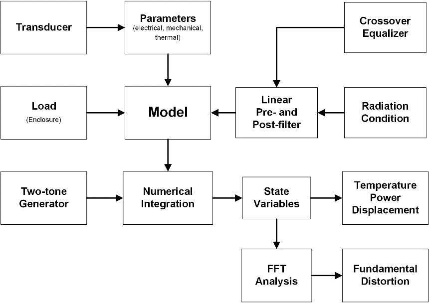
Simulation

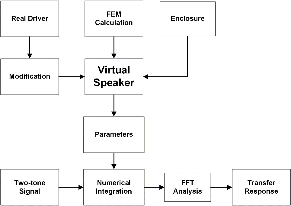
Whereas the prediction uses the parameters of a real loudspeaker system one may also simulate the behavior of a virtual loudspeaker before the first prototype has been finished. The parameters may be produced by FEM-calculations or by simply modifying the parameters of an existing speaker to assess design choices.

The simulation of the transfer response can be performed in the following way:

Simulation of virtually modified transducers and prediction of frequency dependent responses

Separation

To find the dominant source of distortion and to investigate design choices the following nonlinearities might be enabled or disabled during simulation:

• motor nonlinearity due to \(Bl(x)\)

• mechanical suspension nonlinearity due to \(K_{\text{ms}} (x)\)

• inductance nonlinearity due to \(L_{\text{e}} (x)\)

• nonlinearity of para-inductance \(L_2(x),L_3(x)\)

• nonlinearity of resistance \(R_2(x), R_3(x)\) due to eddy current losses

• reluctance force \(F_{\text{m}}\) (electromagnetic drive)

• adiabatic compression in enclosure \(K_{\text{ab}} (p_{\text{box}})\)

• adiabatic compression of rear enclosure \(K_{\text{r}} (p_{\text{rear}})\)

• nonlinearity of port losses \(R_{\text{ap}} (v_{\text{p}})\)

• passive radiator stiffness nonlinearity \(K_{\text{mr}} (x_{\text{r}})\)

• radiation distortion (Doppler effect)

Initial Conditions

The displacement at the beginning of the numerical integration may be specified by the user to investigate the stability of the driver. Performing two simulations with varied initial displacement \((x(t=0)=x_{\text{max}}\) and \(x(t=0)==x_{\text{max}})\) reveal critical frequencies where the driver bifurcates into different solutions.

Heating of the Coil

Simultaneously with the solution of the electrical, mechanical and acoustical system the instantaneous voice coil temperature will be predicted by using the electrical input power \(P\) and the thermal parameters. The user may investigate the short term and the long term thermal performance of the driver. For the short term performance it is assumed that the voice coil temperature has reached steady state while the magnet is still cold. The long term performance is simulated assuming both voice coil and magnet are hot and in thermal equilibrium.

Different Solvers

Different algorithms for the numerical integration are provided. The user may choose either a fast solver with fixed step size or a more sophisticated solver with step size control giving higher precision. If the system behaves stiff (model contains time constants of very different magnitude) a special (implicit) solver that can cope with the problem will be used in both cases.

Post processing

The steady state driver variables are subject to a FFT analysis. Since the frequencies \(f_1\) and \(f_2\) of the excitation tones corresponds with the FFT length additional windowing of the time signal can be omitted. This reveals the spectral components without any smearing effects.

Full Resolution Spectrum of far field Pressure

Property Pages

After activating the SIM module, you can open the property pages. These pages represent the setup parameters for simulation and result analysis.

Property Page

Function

Info

The Info page allows the user to change the name of the measurement and to add a comment to the measurement.

Driver

The Driver page contains special transducer parameters that have to be provided by the user.

Stimulus

The Stimulus page is used to specify the stimulus (excitation signal) for the simulation.

Transducer

This page contains the linear and nonlinear driver parameters. The individual model nonlinearities can be switch on or off and the shape of the nonlinearities can be edited

System

In the System page the enclosure in which the driver is embedded, the pre-filter (describing e.g. the cross-over) and the cone-radiation-room model is specified.

Thermal

This page is used to specify the parameters of the nonlinear thermal model and the mode for thermal simulation.

Im/Export

This page is used to import/export the SIM/DIS setup from/to clipboard and to import results from other modules. Furthermore and the numerical simulation mode the initial conditions can be specified.

Display

This page controls the contents of several result charts. The user can select the signal, the sweep point and the order of distortion. Furthermore, the result plots can be customized here.

INFO Page

The Info page allows the user to change the name of the operation and to add a comment to the operation (comments may be included in the report file).

DRIVER Page

The Driver page contains special transducer parameters that have to be provided by the user.

\(S_{\text{d}}\) in \(\text{cm}^2\)

The diaphragm area is the effective projected surface area of the driver diaphragm

\(d_{\text{d}}\) in cm

Diaphragm diameter of the driver

\(Z_{\text{n}}\) in Ohm

Nominal impedance of the driver

\(P_{\text{e}}(max)\) in W

Maximal nominal input power

Material of voice coil

The kind of material (copper, aluminum) used for the voice coil has to be specified if known. This information is used to identify the increase of voice coil temperature from the variations of the voice coil resistance.

STIMULUS Page

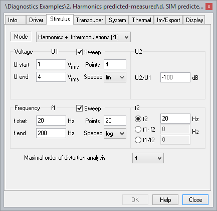
The Stimulus page gives access to the parameters used for controlling the voltage and the frequency of the excitation signal. An “array” of voltage-frequency points can be specified. The SIM will sweep through this array and simulate the distortion for each voltage-frequency point.

Mode

There are four different measurement modes. (n denotes the maximal order of distortion analysis)

1. Harmonics

   Harmonic distortions are simulated only. Maximal sweep frequency \(f_{\text{end}}\) is \(24 \text{kHz}\ /\ n\) .

2. Harmonics + Intermodulations (f1)

   Harmonic and intermodulation distortion centered around the excitation frequency \(f_1\) are simulated. Maximal sweep frequency \(f_{\text{end}}\) is the minimum of \(24 \text{kHz}\ /\ n\) and \(24 \text{kHz}-(n-1)\cdot f_2\) .

3. Harmonics + Intermodulations (f2)

   Harmonic and intermodulation distortion centered around the excitation frequency \(f_2\) are simulated. Maximal sweep frequency \(f_{\text{end}}\) is the minimum of \(24 \text{kHz}\ /\ n\) and \(24 \text{kHz}-(n-1)\cdot f_2\) .

4. Intermodulation (f1)

   Intermodulation distortion only centered around the excitation frequency \(f_1\) are simulated. Maximal sweep frequency \(f_{\text{end}}\) is \(24 \text{kHz}-(n-1)\cdot f_2 ` . This often allows higher frequencies :math:`f_{\text{end}}\) as harmonic frequencies are not considered.

Voltage U1

If the checkbox Voltage U1 Sweep is selected, the loudspeaker will be simulated sequentially for several voltages of the first excitation tone. The user can specify the first voltage \(\textbf{U}_{\text{start}}\), the last voltage \(\textbf{U}_{\text{end}}\) and the number of points covered by the voltage sweep (Points) as well as the spacing (linear or logarithmic) of the sweep points (Spaced).

Voltage: U2/U1

The voltage \(U_2\) of the second excitation tone is coupled to the voltage \(U_1\) of the first tone. The ratio \(U_2/U_1\) has to be specified in dB.

Frequency f1

If the checkbox Frequency f1 Sweep is selected the loudspeaker will be simulated sequentially for several frequencies of the first excitation tone. The user can specify the first frequency \(\textbf{f}_{\text{start}}\), the last frequency \(\textbf{f}_{\text{end}}\) and the number of points covered by the frequency sweep (Points) as well as the spacing (linear or logarithmic) of sweep points (Spaced).

Frequency f2

There are different ways to specify the frequency \(f_2\) of the second excitation tone:

1. \(\textbf{f}_2:\) The frequency of the second excitation tone is held constant during the sweep of \(f_1\). This mode allows to generate very critical stimuli for most transducers. Selecting may represent a bass tone producing \(f_2\lt f_1,f_2\) large voice coil displacement and \(f_1\) represents any audio component (voice) in the pass band of the transducer.

2. \(\textbf{f}_1-\textbf{f}_2:\) The distance \(f_1-f_2\) between both excitation frequencies is held constant during the sweep of \(f_1\). This mode produces difference intermodulations at the same frequency independent of \(f_1\).

3. \(\textbf{f}_1/\textbf{f}_2:\) The ratio \(f_1/f_2\) is held constant during the sweep of \(f1\). Selecting \(f_2\gt f_1\) and using a fractional ratio (e.g. 0.18) this mode avoids interference between the harmonic and intermodulation distortion components.

Maximal order of distortion analysis

Distortions will be calculated up to the specified order (2, 3 … 16).

TRANSDUCER Page

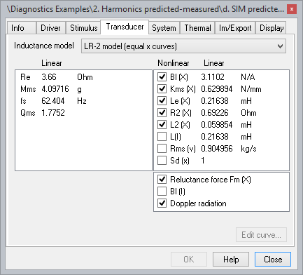
The transducer page is used for specifying the linear and nonlinear transducer parameters. The individual nonlinearities can be switched on and off. The shape of the nonlinearities can be edited either using a curve editor or by altering the power series coefficients. The nonlinear model is described in detail in the section sim2-reference | Theory | Transducer Modeling in the chapter SIM Reference.

Inductance Model

Different inductance models can be used for simulation. The simplest model is the Single Inductor where the inductance is modeled by \(L(s)*s\cdot L_{\text{e}}\)

The LR-2 and the LR‑3 model are more complex models. The inductance is modeled by \(L(s)=s\cdot L_{\text{e}}+s\cdot L_2//R_2\) and \(L(s)=s\cdot L_{\text{e}}+s\cdot L_2//R_2+s\cdot L_3//R_3\) respectively.

Linear Transducer Parameters

The values of the linear transducer parameters are specified in the table Linear. If one parameter value is changed all dependent parameters are recalculated automatically.

\(R_{\text{e}}\) in \(\text{Ohm}\)

DC resistance of voice coil

\(M_{\text{ms}}\) in \(\text{g}\)

mechanical moving mass including air load

\(R_{\text{ms}}\) in \(\text{Ns/m}\)

mechanical resistance of suspension losses

\(f_{\text{s}}\) in \(\text{Hz}\)

driver resonance frequency

\(Q_{\text{ms}}\)

mechanical loss factor of driver in free air considering \(R_{\text{ms}}\) only

The parameters are linked by the following equations:

\[f_{\text{s}}=\frac{1}{2\pi\sqrt{\frac{M_{\text{ms}}}{K_{\text{ms}}}}}\]

\[Q_{\text{ms}}=2\pi\frac{M_{\text{ms}}}{R_{\text{ms}}}\]

Bl(X)

If the checkbox is selected the nonlinear dependence of the force factor on the displacement x is incorporated into the driver model. Otherwise \(Bl(x)*Bl(x*0)\) is considered to be independent of \(x\). The value right of the checkbox is the small signal parameter \(Bl(x=0)\) which can be modified by double clicking. The Edit curve… button opens a dialog where the shape of the \(Bl(x)\) nonlinearity can be edited. See How to edit the nonlinear parameters later in this section for further information. The result window \(Bl(x)\) shows the specified curve \(Bl\) versus \(x\).

Kms(X)

If selected the nonlinear dependence of mechanical compliance on the displacement \(x\) is incorporated into the driver model. Otherwise \(K_{\text{ms}}(x)*K_{\text{ms}}(x*0)\) is considered to be independent of \(x\). The value right of the checkbox is the small signal parameter \(K_{\text{ms}}(x)=K_{\text{ms}}(x=0)\) which can be modified by double clicking. The Edit curve… button opens a dialog where the shape of the \(K_{\text{ms}}(x)\) nonlinearity can be edited. See How to edit the nonlinear parameters later in this section for further information. The result window \(\textbf{Kms}\textbf{(x)}\) shows the specified curve \(K_{\text{ms}}\) versus \(x\).

Le(X)

If selected the nonlinear dependence of the voice coil inductance on the displacement \(x\) is incorporated into the driver model. Otherwise \(L_{\text{e}}(x)*L_{\text{e}}(x*0)\) is considered to be independent of \(x\). The value right of the checkbox is the small signal parameter \(L_{\text{e}}(x=0)\) which can be modified by double clicking. The Edit curve… button opens a dialog where the shape of the \(L_{\text{e}}(x)\) nonlinearity can be edited. See How to edit the nonlinear parameters later in this section for further information. The result window \(\textbf{Le}\textbf{(x)}\) shows the specified curve \(L_{\text{e}}\) versus \(x\).

R2(X)

If selected the nonlinear dependence of resistance due to eddy currents on the displacement \(x\) is incorporated into the driver model. Otherwise \(R_2(x)*R_2(x*0)\) is considered to be independent of \(x\). The value right of the checkbox is the small signal parameter \(R_2(x=0)\) which can be modified by double clicking. The Edit curve… button opens a dialog where the shape of the \(R_2(x)\) nonlinearity can be edited. See How to edit the nonlinear parameters later in this section for further information. The result window \(\textbf{R2},\textbf{R3}\textbf{(x)}\) shows the specified curve \(R_2\) versus \(x\).

L2(X)

If selected the nonlinear dependence of the para inductance on the displacement \(x\) is incorporated into the driver model. Otherwise \(L_2(x)*L_2(x*0)\) is considered to be independent of \(x\). The value right of the checkbox is the small signal parameter \(L_2(x=0)\) which can be modified by double clicking. The Edit curve… button opens a dialog where the shape of the \(L_2(x)\) nonlinearity can be edited. See How to edit the nonlinear parameters later in this section for further information. The result window \(\textbf{L2},\textbf{L3}\textbf{(x)}\) shows the specified curve \(L_2\) versus \(x\).

R3(X)

If selected the nonlinear dependence of resistance due to eddy currents on the displacement \(x\) is incorporated into the driver model. Otherwise \(R_3(x)*R_3(x*0)\) is considered to be independent of \(x\). The value right of the checkbox is the small signal parameter \(R_3(x=0)\) which can be modified by double clicking. The Edit curve… button opens a dialog where the shape of the \(R_3(x)\) nonlinearity can be edited. See How to edit the nonlinear parameters later in this section for further information. The result window \(\textbf{R2},\textbf{R3}\textbf{(x)}\) shows the specified curve \(R_3\) versus \(x\).

L3(X)

If selected the nonlinear dependence of the para inductance on the displacement \(x\) is incorporated into the driver model. Otherwise \(L_3(x)*L_3(x*0)\) is considered to be independent of \(x\). The value right of the checkbox is the small signal parameter \(L_3(x=0)\) which can be modified by double clicking. The Edit curve… button opens a dialog where the shape of the \(L_3(x)\) nonlinearity can be edited. See How to edit the nonlinear parameters later in this section for further information. The result window \(\textbf{L2},\textbf{L3}\textbf{(x)}\) shows the specified curve \(L_3\) versus \(x\).

Reluctance force Fm(X)

If selected the reluctance force

\[F_{\text{m}}(x,i,i_2,i_3)\approx -\frac{i(t)^2}{2}\frac{\partial L_{\text{e}}(x)}{\partial x}- \frac{i_2(t)^2}{2}\frac{\partial L_2(x)}{\partial x}-\frac{i_3(t)^2}{2}\frac{\partial L_3(x)}{\partial x}\]

is incorporated into the driver model (see section sim2-reference | Theory | Transducer Modeling in the chapter SIM Reference).

Flux modulation F(X)

If selected the flux modulation

\[F(x)=f_0+f_1\cdot x\]

is incorporated into the driver model. The coefficients \(f_0\) and \(f_1\) can be edited by clicking at the Edit curve… button. This will open a dialog where the coefficients \(f_0\) and \(f_1\) can be entered. Furthermore a current \(I_0\) can be specified which is used to show the effect of the flux modulation to the force factor in result window \(\textbf{Bl(x)}\). Right click at result window \(\textbf{Bl(x)}\) and select Customization Dialog … ‣ Subsets . This will open a dialog. Select all subsets. The result window \(\textbf{Bl(x)}\) shows now the two additional curves

\[Bl(x,I_0)=Bl(x)\cdot \left[ 1+I_0\cdot F(x)\right]\]

\[Bl(x,-I_0)=Bl(x)\cdot \left[ 1-I_0\cdot F(x)\right]\]

They depict the modulation of the force factor caused by positive and negative currents.

Doppler radiation

If selected the Doppler Effect is incorporated into the model.

SYSTEM Page

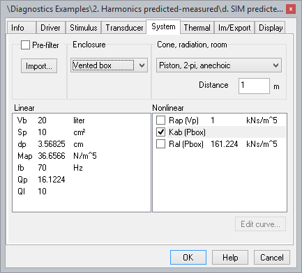
In the System page the enclosure in which the driver is embedded, the pre-filter (describing e.g. the cross-over) and the model for cone, radiation and room is specified.

Enclosure

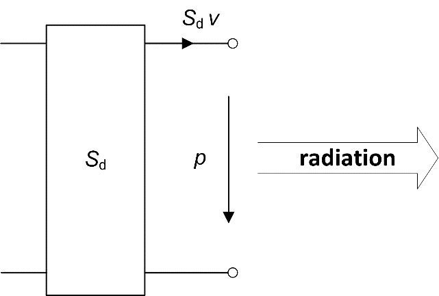
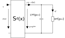
Type of enclosure in which the driver is supposed to be mounted. Six different enclosures are supported. The schematics show the acoustical part of the corresponding model. For detailed information, see section #sim2-reference | Theory |# Transducer Modeling.

Driver in baffle

No additional enclosure modeling is applied.

Closed box

Vented box

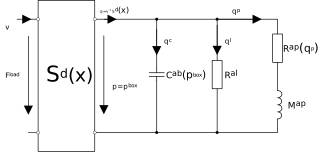
Passive radiator

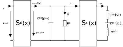
Bandpass

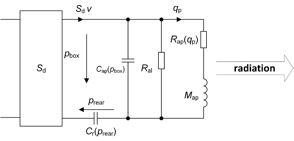
General Enclosure Definition

The impedance \(Z\) of the acoustic system of a general enclosure can be freely specified. For this the coefficients of 10 second order continuous filters connected in series can be adjusted to match the desired dynamics. The impedance can be specified either as electrical \((Z_{\text{e}})\), mechanical \((Z_{\text{m}})\) or acoustical \((Z_{\text{a}})\) impedance. Click the Edit… button to open a dialog where you can enter the filter coefficients.

Electrical Impedance *Ze*

Mechanical Impedance *Zm*

Acoustical Impedance *Za*

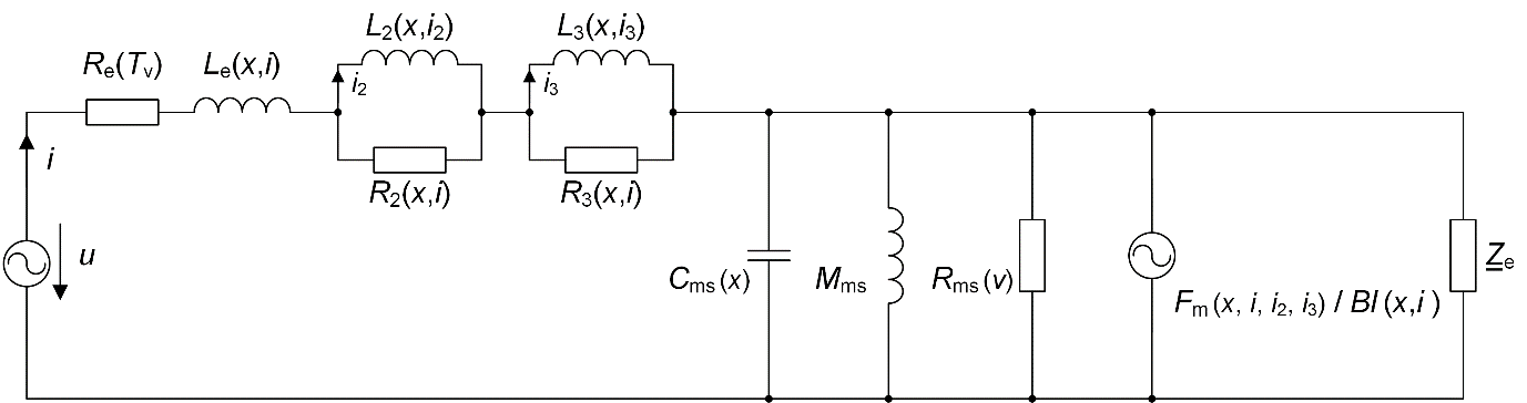
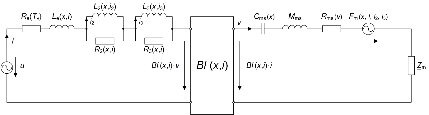
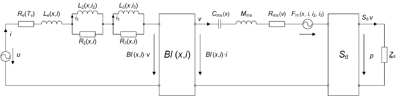
Linear Enclosure Parameters

The values of linear enclosure parameters are specified in the tables Linear and Nonlinear. If one parameter value is changed all dependent parameters are recalculated automatically.

\(v_{\text{b}}\) in \(liter\)

Volume of air in enclosure Note: \(v_{\text{b}}\) directly affects the acoustical compliance \(C_{\text{ab}}\) .

\(v_{\text{r}}\) in \(liter\)

Volume at rear enclosure in bandpass system Note: \(v_{\text{r}}\) directly affects the acoustical compliance \(C_{\text{r}}\) .

\(S_{\text{p}}\) in \(\text{cm}^2\)

Area of port

\(d_{\text{p}}\) in cm

Equivalent diameter for circular \(S_{\text{p}}\)

\(S_{\text{r}}\) in \(\text{cm}^2\)

Area of passive radiator

\(d_{\text{r}}\) in cm

Equivalent diameter for circular \(S_{\text{r}}\)

\(M_{\text{ap}}\) in \(\text{kg}/{\text{m}}^4\)

Acoustic mass of air moved in vent

\(M_{\text{mr}}\) in g

Mechanical moving mass of passive radiator

\(R_{\text{al}}\) in \(\text{kNs}/{\text{m}}^5\)

Acoustic resistance of enclosure losses due to leakage

\(f_{\text{b}}\) in Hz

Resonance frequency of enclosure

\(f_{\text{c}}\) in Hz

Resonance frequency of the closed box system

\(Q_{\text{p}}\)

Loss factor of the acoustic system at \(f_{\text{b}}\) considering vent/passive radiator losses

\(Q_{\text{l}}\)

Loss factor of the acoustic system at \(f_{\text{b}}\) considering leakage losses

\(Q_{\text{tc}}\)

Loss factor of the Resonance frequency of the closed box system at \(f_{\text{c}}\)

The parameters of the closed box are linked by the following equations:

\[f_{\text{c}}=\frac{1}{2\pi\sqrt{M_{\text{ms}}\cdot C_{\text{mt}}(0)}}\]

\[Q_{\text{tc}}=\frac{1}{2\pi\cdot f_{\text{c}}(p_{\text{box}},x)\cdot S_{\text{d}}\cdot C_{\text{mt}}(0) \cdot R_{\text{atc}}(0)}\]

\[C_{\text{mt}}(x)=\frac{1}{K_{\text{ms}}(x)+\mathrm{S}_{\text{d}}^{2}\cdot \frac{1}{C_{\text{ab}}(0)}}\]

\[R_{\text{atc}}(x)=\frac{1}{\frac{R_{\text{ms}}(x)}{S_{\text{d}}}+\frac{Bl^2(x)}{R_{\text{e}}\cdot S_{\text{d}}}}\]

The parameters of the vented box and the bandpass are linked by the following equations:

\[f_{\text{b}}=\frac{1}{2\pi\sqrt{M_{\text{ap}}\cdot C_{\text{ab}}(0)}}\]

\[Q_{\text{p}}=\frac{1}{2\pi f_{\text{b}}\cdot C_{\text{ab}}(0)\cdot R_{\text{ap}}(0)}\]

\[Q_1=2\pi f_{\text{b}}\cdot C_{\text{ab}}(0)\cdot R_{\text{al}}\]

where \(C_{\text{ab}}(0)=v_{\text{b}}/\gamma\cdot p_0\) with \(\gamma=1.4\) and \(P_o=101,3\) \(\text{kN}/\text{m}^2\)

The following relations hold for the linear parameters of the passive radiator:

\[f_{\text{b}}=\frac{1}{2\pi\sqrt{M_{\text{ar}}\cdot \frac{C_{\text{ab}}(0) \cdot C_{\text{ar}}(0)}{C_{\text{ab}}(0)+C_{\text{ar}}(0)}}}\]

\[Q_{\text{p}}= \frac{2\pi f_{\text{b}}\cdot \mathrm{M}_{\text{ar}}} {\mathrm{R}_{\text{ar}}}\]

\[Q_l=2\pi f_{\text{b}}\cdot C_{\text{ab}}(0)\cdot R_{\text{al}}\]

where

• \(C_{\text{ab}}(0) = \frac{v_{\text{b}}} {\gamma\cdot p_0}\)

• \(C_{\text{ar}}(0) = \frac{\mathrm{S}_{\text{r}}^{2}} {K_{\text{mr}}(0)}\)

• \(R_{\text{ar}}(0) = \mathrm{S}_{\text{r}}^{2} \cdot R_{\text{mr}}(0)\)

• \(M_{\text{ar}}(0) = \mathrm{S}_{\text{r}}^{2} \cdot M_{\text{mr}}(0)\)

Note

SIM-AUR and LSIM are using an differing naming convetion for passive radiator parameter. SIM2 indicates the passive radiator with \(r\) for radiator. SIM-AUR and LSIM are using the common used \(p\) for passive radiator.

Rap(Vp)

If selected the nonlinear dependence of the vent losses on the velocity \(v_{\text{p}}\) is incorporated into the model. Otherwise \(R_{\text{ap}} (v_{\text{p}})* R_{\text{ap}} (v_{\text{p}}*0)\) is considered to be independent of \(v_{\text{p}}\). The value right of the checkbox is the small signal parameter \(R_{\text{ap}} (v_p=0)\) which can be modified by double clicking. The Edit curve… button opens a dialog where the shape of the \(R_{\text{ap}} (v_p)\) nonlinearity can be edited. See How to edit the nonlinear parameters later in this section for further information. Instead of a power series with freely defined coefficients the theoretical characteristics

\[R_{\text{ap}} (v_{\text{p}}) = R_{\text{ap}} (v_{\text{p}}=0) + \frac{\rho}{2\cdot S_{\text{p}}} \cdot \left| v_{\text{p}} \right|\]

\(\rho\) – density of air, \(S_{\text{p}}\) – port area

can be used by selecting Theoretical characterstic on page Graphic.

The result window Rap(Vp) shows the specified curve \(R_{\text{ap}}\) versus \(v_{\text{p}}\).

Kmr(Xr)

If selected the nonlinear dependence of the passive radiator suspension stiffness on the passive radiator displacement \(x_{\text{r}}\) is incorporated into the model. Otherwise \(K_{\text{mr}} (x_{\text{r}})*K_{\text{mr}}(x_r*0)\) is considered to be independent of \(x_{\text{r}}\). The value right of the checkbox is the small signal parameter \(K_{\text{mr}} (x_r=0)\) which can be modified by double clicking. The Edit curve… button opens a dialog where the shape of the \(K_{\text{mr}} (x_r)\) nonlinearity can be edited. See How to edit the nonlinear parameters later in this section for further information. The result window Kmr(Xr) shows the specified curve \(K_{\text{mr}}\) versus \(x_r\).

Kab (Pbox)

If selected the nonlinear dependence of the acoustic stiffness of air in enclosure on the sound pressure \(p_{\text{box}}\) is incorporated into the model. Otherwise \(K_{\text{ab}}(p_{\text{box}}*0)\) is considered to be independent of \(p_{\text{box}}\) .

Kr (Prear)

If selected the nonlinear dependence of the acoustic stiffness of air in rear enclosure on the sound pressure \(p_{\text{rear}}\) is incorporated into the model. Otherwise \(K_{\text{r}} (p_{\text{rear}}*K_{\text{r}}) (p_{\text{rear}}*0)\) is considered to be independent of \(p_{\text{rear}}\) .

Pre-filter

The two=tone excitation signal \(U(f)\) can be filtered before it is passed on to the driver. This way the effect of a crossover can be simulated. See section SIM Reference ‣ Theory ‣ State Space ‣ Equation ‣ Prefilter for further information.

The pre-filter is activated by selecting the checkbox Pre-Filter. Clicking at the Import… button opens a dialog where the filter transfer function \(H_{\text{pre}}(f)\) can be imported from the clipboard. There are two formats supported. The first format is a two-column matrix where the first column gives the frequency in Hz and the second the magnitude of \(H_{\text{pre}}(f)\) in dB. Furthermore a three-column matrix is supported where the first column contains the frequency in Hz the second the magnitude of \(H_{\text{pre}}(f)\) in dB and the third the phase in degree. See section Curve import and export later in the Reference for more information about the import format.

Cone, Radiation, Room

Two different ways to calculate the sound pressure in the far field are supported. See section SIM Reference ‣ Theory ‣ State Space Equation ‣ Cone, Radiation, Room for further information.

1. Piston, \(\textbf 2 \pi (\textbf 4 \pi)\), anechoic

If one of these options is selected a simple model that assumes “ideal” 2π or 4π-space radiation without any deterioration of the rooms is used. The user has to specify the distance between diaphragm and listening position. In the model equations this distance is denoted by \(r\) and it is assumed that the listening position is on-axis.

2. Import overall system response

If this option is selected the frequency response \(H_{\text{total}}(f)=P_{\text{far}}(f)/U(f)\) for the overall system (measured or synthesized) can be imported to calculate the sound pressure. Rooms of small and medium size affect the far field sound pressure signal considerably. The transmission varies considerably with frequency and listening position and the relationship between frequency and transmission is usually very complicated. However, this relationship can easily be measured for instance with the TRF module of the Klippel R&D System. Using a measured transfer function \(H_{\text{total}}(f)\) leads to simulation results that reflect the influence of the cone breakup modes, the radiation and the particular room. This way the sound pressure for the actual listening environments can be simulated and easily compared with the measured sound pressure.

For more information on the underlying principle, please see section SIM_Reference ‣ Theory ‣ State Space Equation ‣ Import of total frequency response

Clicking at the Import… button opens a dialog where the transfer function \(H_{\text{total}}(f)\) can be imported from the clipboard. There are two formats supported. The first format is a two-column matrix where the first column gives the frequency in Hz and the second the magnitude of \(H_{\text{total}}(f)\) in dB. Furthermore a three-column matrix is supported where the first column contains the frequency in Hz, the second the magnitude of \(H_{\text{total}}(f)\) in dB and the third the phase in degree. See section Importing curves later in the Reference for more information about the required data format.

How to edit the nonlinear parameters

Clicking at the Edit curve… button in the property pages Transducer and System opens a dialog where the shape of the nonlinear parameters can be modified. The dialog has three pages. In the Regular and the Special page, the corresponding power series coefficients can be imported and modified. The Graphic page provides an editor that allows to edit the curve properties graphically.

Regular

This page gives access to the coefficients of the ordinary power series

\[Y(x)=Y(x=0)+b_1x+b_2x^2+b_3x^3+...\]

where \(Y(x)\) symbolizes \(Bl(x), K_{\text{ms}}(x), L_{\text{e}}(x), R_{\text{ap}} (v_{\text{p}})\), etc.

Special

This page gives access to the coefficients of a modified power series that is more suited to the driver physics

\(Y(x)=b_0K\) if \(K\ge 1\)

\(Y(x)=\frac{b_0}{2-K}\) if \(K\lt 1\)

with \(K = 1 + b_{1}x + b_{2}x^{2} + b_{3}x^{3} + \ldots\) and \(b_0=Y(x=0)\)

\(Y(x)\) symbolizes \(Bl(x), K_{\text{ms}}(x), L_{\text{e}}(x), R_{\text{ap}}(v_p)\), etc.

Graphic

The Graphic page provides five sliders for modifying the curve shape graphically.

Graphical Editor for Nonlinerarities

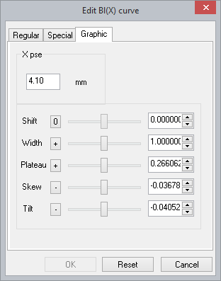
1. Shift controls the horizontal shift of curve. It can be used to center the nonlinearity by shifting the curve to maximum to \(x=0\) .

2. Width is the width of the curve. The curve can be made wider or narrower. Use the slider to adjust the point at which the force factor drops to 50 percent. This corresponds to the (half) gap width (underhung configuration) /voice coil height (overhang configuration) .

3. Plateau controls the region around the rest position. The slider changes its shape from plateau like to peak like.

4. Skew controls the asymmetry of the curve referred to axis that runs through the maximal curve value. Referred to this axis the curve can be made more symmetric/skewed.

5. Tilt controls the overall slope of the curve. The slope can be positive or negative. The slope is an asymmetric parameter.

To change the slider range drag the slider to the boundary and hold it. Holding the slider at the right (left) boundary will shift the range upwards (downwards). The shift can be accelerated by pressing the SHIFT button simultaneously. The button left of the slider is for changing the sign of the curve parameter. Pressing the button will toggle the sign between positive, negative and zero. If zero is selected the parameter value is set to zero. Alternatively edit boxes right of the sliders can be used to enter the curve parameters directly.

While adjusting curve shapes it is sometimes useful to compare with the original curve. In order to view the original curve open the curve editor and right click at the result window. Choose Customization Dialog… ‣ Subsets and add the Original subset to the already selected subsets.

Xpse, Vp pse, Xr pse

Both the regular and the special power series are expanded over the range \(\pm \textbf{X}_{pse}\) (or \(\pm \textbf{Vp}_{pse}, \pm \textbf{Xr}_{pse}\) respectively). This is the range for which the power series is valid. If for instance the power series is imported from the LSI module \(\textbf{X}_{pse}\) is the displacement range covered during measurement.

Note

Pse stands for power series expansion.

Note

Both the regular and the special power series may behave quite differently outside the expansion range. Therefore a warning message will be generated if \(\left| x \right|, \left| v_{\text{p}} \right|\) or \(\left| x_{\text{r}} \right|\) exceeds \(X_{pse}, Vp_{pse}\) or \(Xr_{pse}\) during simulation. If you want to enlarge the expansion range (in order to simulate higher excitation levels) make sure that the power series is valid over the full range. Check the result windows of all relevant nonlinear parameters. There the curves are displayed over the full expansion range.

Order

The power series order can be selected with the dropdown box Order. If the order of an existing power series is modified new coefficients are calculated to fit the original curve shape.

Shift

The curve can be shifted horizontally. This is for instance useful to center the force factor or stiffness curve by shifting the curve maximum / minimum to \(x=0\). The shift is activated by clicking the Set button. The default shift value will move the curve maximum / minimu to \(x=0\). New power series coefficients will be calculated to fit the shifted curve. The Shift operation can be performed repeatedly.

Center

For the Bl(x), Kms(x) and the Rms(v) nonlinearity, the curve can be centered automatically by pressing the Center button. This will search for the maximum of the nonlinearity and set the shift accordingly.

Importing curves

Clicking the Import curve… button opens a dialog where a curve can be imported from the clipboard in order to calculate the corresponding power series coefficients. For this the curve must be represented as two-column matrix where the first column gives the x-values and the second the y-values. See section Curve Im/Export later in the Reference for more information about the import format.

THERMAL Page

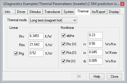
This page is used to specify the parameters of the nonlinear thermal model and the mode for thermal simulation. See section SIM Reference ‣ Theory ‣ Transducer Modeling ‣ Thermal Modeling for further information about the thermal model.

Thermal mode

Simultaneously with the solution of the electrical, mechanical and acoustical system the thermal heating of the transducer will be predicted. Three different modes are supported. All simulate steady state thermal conditions:

1. No simulation The thermal simulation is switched off. Voice coil and magnet are assumed to be at ambient temperature.

2. Short term (magnet cold) This mode simulates the short term thermal behavior. It is assumed that the voice coil temperature has reached steady-state while the magnet is still cold \((\Delta T_{\text{m}}=\Delta T_{\text{g}}=0)\) .

3. Long term (magnet hot) This mode simulates the long term thermal behavior. Both voice coil and magnet temperature are assumed to be hot and in steady-state.

Thermal parameters

\(R_{\text{tv}}\)

thermal resistance of path from coil to pole tips and magnet surface

\(R_{\text{tm}}\)

thermal resistance of path from magnet to ambient air

\(R_{\text{tg}}\)

thermal resistance of path from pole tips to magnet and frame

\(R_{\text{ta}} (x)\)

thermal resistance of path from air in the gap to ambience due to convection cooling

\(R_{\text{tc}} (v)\)

thermal resistance of path from coil to air in the gap due to convection cooling

\(R_{\text{tt}} (v)\)

thermal resistance of path from air in the gap to the magnet structure due to convection cooling

\(r_{\text{x}}\)

convection cooling parameter considering the effect of cone displacement

\(r_{\text{v}}\)

convection cooling parameter considering the cone velocity

\(r_{\text{b}}\)

convection cooling parameter considering the cone velocity

\(\alpha\)

factor describing the distribution of heat caused by eddy currents on voice coil and magnet

The thermal model can be simplified by switching off the thermal resistances \(R_{\text{ta}} (x), R_{\text{tc}} (v), R_{\text{tt}} (v), R_{\text{tg}}\) and the direct heating due to eddy currents (\(\alpha\)). This is useful if the corresponding thermal parameters are not known.

The thermal parameters \(R_{\text{tv}}, R_{\text{tm}}\) and \(r_{\text{v}}\) can be measured with and imported from the LSI module (see Im/Export-Page). The PWT power test module measures the parameter \(R_{\text{tv}}, R_{\text{tm}}, r_{\text{v}}\) and α. They can be imported to SIM via the Im/Export-Page.

IM/EXPORT Page

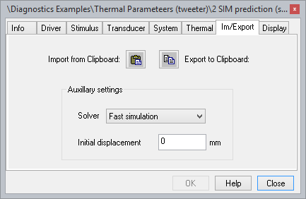
This page is used to import parameters from other Klippel modules, as well as setting the solver mode and an initial displacement. All modules supporting import and export functionality are documented in the section Supported Modules for Im/Export.

Solver

The solver for the numerical solution of the system equations can be chosen by the user. If Fast Simulation is selected a solver without step size control will be used. This solver is very fast and will calculate in most cases the exact speaker states. In some few cases the precision will suffer and a more sophisticated solver with step size control has to be used (Precise Simulation).

Initial Displacement

The displacement of the voice coil at the beginning of the numerical integration can be specified by the user to e.g. investigate the driver stability.

DISPLAY Page

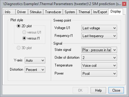
Plot style: 2D

If selected, all 3D result windows are switched to 2D=mode. The distortions can be plotted either versus excitation voltage \(U_1\) (versus U1) or versus excitation frequency \(f_1\) (versus f1) . The windows will be empty if no voltage sweep was performed (see property page STIMULUS) and versus U1 is selected of if no frequency sweep was performed and versus f1 was selected.

Plot style: 3D

If selected the distortions are plotted versus excitation voltage and frequency. The windows will be empty if either no voltage sweep or no frequency sweep was performed (see property page STIMULUS).

Plot style: Y-axis

This combo box is for adjusting the spacing of the y‑axis of the result windows

• Fundamental

• Harmonic (n)

• Diff. Intermod (n)

• Sum. Intermod (n) and

• Peak + Bottom.

First, linear (Lin) or logarithmic (Log) spacing can be chosen. If Auto is selected the spacing is chosen automatically. In order to visualize power compression effects the automatic spacing is selected according to the spacing of the voltage sweep selected in property page Stimulus. In case of no power compression simulation results for different drive levels will be displayed as equidistant curves. Any power compression will disturb this equidistant spacing. The y-axis spacing (Lin/Log/Auto) can be selected independently for the individual speaker states signals.

Plot style: Distortion

This combo box controls the display of the relative harmonic and intermodulation distortion. The relative distortion can be displayed either in Percent or in dB.

Voltage U1

Determines sweep voltage \(U_1\) for which the results are to be shown in the result windows

• Table Speakerstates,

• Harmonics, % and

• Fundamental + Harmonics.

In order to not inflate the database size the complete waveform and the according spectra are not stored in the database. However, if you want to view waveform and spectra for a particular sweep point you can repeat the simulation for this single sweep point by pressing the Run button. After the single point simulation has finished waveform and spectra for the selected sweep point can be viewed.

Frequency f1

Determines sweep frequency \(f_1\) for which the results are to be shown in the result windows Table Speakerstates.

In order not to inflate the database size the complete waveform and the according spectra are not stored in the database. However, if you want to view waveform and spectra for a particular sweep point you can repeat the simulation for this single sweep point by pressing the Run button. After the single point simulation has finished, waveform and spectra for the selected sweep point can be viewed.

Signal: State signal

Determines the signal (speaker state) for which the results are to be shown. The user can choose between the eight speaker states

• X – cone displacement

• V – cone velocity

• I – input current

• UL – voltage at terminals

• Xr – displacement passive radiator

• qp – volume velocity in port

• Pbox – pressure in box

• Pfar – pressure in far field

Obviously, Pbox and qp cannot be selected if the driver was supposed to be mounted in a baffle. qp cannot be selected for the closed box and Xr can only be selected for the passive radiator.

Signal: Order of distortion

Determines the order of distortion (2, 3 … \(N\)) for which the results are to be shown in result windows

\(N\) is the Maximal order of distortion analysis specified in property page Stimulus.

• Harmonics (n),

• Diff. Intermod (n) and

• Sum. Intermod (n).

Signal: Temperature

Determines which temperature is shown in result window Temperature. The following temperatures increases can be selected

• Voice coil

• Pole tips

• Magnet

Note that not absolute temperatures but temperature increases are displayed. The increase of the gap and magnet temperature will be zero if Short term (magnet cold) was selected as mode for thermal simulation.

Selecting Re(Tv) shows the DC voice coil resistance that corresponds to the calculated voice coil temperature.

Signal: Power

Determines which power signal is shown in result window Power. The following signals can be selected

• Pcoil - power dissipated in voice coil and former

• Peg - power transferred to the pole tips due to eddy currents

• Pg - power transferred to the pole tips

• Ptv - power transferred to the pole tips from coil

• Pcon - power transferred to the gap air by convection cooling

• Bypass Factor - ratio of power dissipated in coil and power transferred from coil to gap air and pole tips

Result Windows

\(p\) is used in the following sections as an example for any available state.

Harmonics, %

The second-order harmonic distortion

\[d_{\text{h}2}=\frac{p(2f)}{p_{\text{RMS}}}\cdot 100\%\]

third-order harmonic distortion

\[d_{\text{h}3}=\frac{p(3f)}{p_{\text{RMS}}}\cdot 100\%\]

is defined in percent where \(p_{\text{RMS}}\) is the true RMS-value of the analyzed signal. The distortion can either be displayed in percent or in dB (0 dB = 100 %). This selection is made in property page Display.

Total Harmonic, %

The IEC standard 60268 defines the total harmonic distortion

\[d_{\text{ht}}=\frac{\sqrt{p(2f)^2+p(3f)^2+.. +p(nf)^2}}{p_{\text{RMS}}}\cdot 100\%\]

in percent where \(p_{\text{RMS}}\) is the true RMS-value of the analyzed signal. The distortion can either be displayed in percent or in dB (0 dB = 100 %). This selection is made in property page Display.

2nd Harmonic, %

The second-order harmonic component

\[d_{\text{h}2}=\frac{p(2f)}{p_{\text{RMS}}}\cdot 100\%\]

is defined in percent where \(p_{\text{RMS}}\) is the true RMS-value of the analyzed signal. The distortion can either be displayed in percent or in dB (0 dB = 100 %). This selection is made in property page Display.

3rd Harmonic, %

The third-order harmonic distortion

\[d_{\text{h}2}=\frac{p(2f)}{p_{RMS}}\cdot 100\%\]

is defined in percent where \(p_{\text{RMS}}\) is the true RMS-value of the analyzed signal. The distortion can either be displayed in percent or in dB (0 dB = 100 %). This selection is made in property page Display.

2nd Intermod, %

The IEC standard 60268 defines the second-order modulation distortion (centered around frequency \(f_1\))

\[d_2=\frac{p(f_1-f_2)+p(f_1+f_2)}{p(f_1)}\cdot 100\%\]

in percent. If \(f_1\) and \(f_2\) are exchanged in the above formula it defines the second-order modulation distortion centered around frequency \(f_2\). The distortion can either be displayed in percent or in dB (0 dB = 100 %). This selection is made in property page Display.

3rd Intermod, %

The IEC standard 60268 defines the third-order modulation distortion (centered around frequency \(f_1\))

\[d_2=\frac{p(f_1-2f_2)+p(f_1+2f_2)}{p(f_1)}\cdot 100\%\]

in percent. If \(f_1\) and \(f_2\) are exchanged in the above formula, it defines the third-order modulation distortion centered around frequency \(f_2\). The distortion can either be displayed in percent or in dB (0 dB = 100 %). This selection is made in property page Display.

Modulation

Excited with a two-tone signal the loudspeaker produces modulation distortion caused by amplitude and phase (frequency) modulation. Both modulations will produce difference-tone intermodulation components at frequencies \(f_1-(n-1)f_2\) and summed-tone intermodulation distortion \(f_1+(n-1)f_2\) of \(n^{th}\)-order centered around the voice tone \(f_1\).

Assessing frequency and amplitude modulation distortion

The IEC standard 60268 defines the second=order modulation distortion (centered around frequency \(f_1\))

\[L_{\text{d}2}=20\log_{10} \left( \frac{p(f_1-f_2)+p(f_1+f_2)}{p(f_1)} \right)\]

in decibels and the third-order modulation distortion (centered around frequency \(f_1\))

\[L_{\text{d}3}=20\log_{10} \left(\frac{p(f_1-2f_2)+p(f_1+2f_2)}{p(f_1)}\right)\]

in decibels. If \(f_1\) and \(f_2\) are exchanged in the above formulas they define the modulation distortion centered around frequency \(f_2\).

Summarizing the \(2^{nd}\) and \(3^{rd}\)-order modulation distortion we get the modulation distortion

\[L_{\text{dm}}=20\log_{10}\left( 10 ^{L_{\text{d}2}}/_{20}+10 ^{L_{\text{d}3}}/_{20} \right)\]

Assessing amplitude modulation only

The distortion of the pure amplitude modulation can be assessed separately by measuring the variation of the envelope of the high-frequency tone \(f_1\) (voice tone).

The envelope \(E[t]\) of the voice tone \(f_1\) is derived from the time sound pressure signal \(p[t]\) by considering the fundamental of \(f_1\) and the summed-tone and difference-tone intermodulation \(f_1-(n-1)f_2\) and \(f_1+(n-1)f_2\), respectively, with \(2\lt n\lt N\) .

Calculating the averaged envelope over one period \(T\)

\[\overline{E}=\frac{1}{T}\int_{T}^{}E[t]dt\]

we define the RMS-amplitude modulation distortion

\[d_{\text{AMD}}=\frac{\sqrt{\frac{2}{T}\int_{T}^{}(E[t]-\overline{E})dt}}{\overline{E}}\cdot 100\%\]

expressed in percent or in decibels

\[L_{\text{AMD}}=20\log_{10}(\frac{d_{\text{AMD}}}{100})\]

Fundamental + Harmonics

The fundamental component

\[L=20\log_{10}(p(f_1))\]

and the \(n^{th}\)-order harmonic distortion (\(n\) =2,3)

\[L_{\text{h}n}=20\log_{10}(p(nf_1))\]

of excitation frequency \(f\) is expressed in dB.

Fundamental

This result window shows the fundamental component versus frequency \(f_1\) and/or voltage \(U_1\) for the signal selected in property page Display. The fundamental can either be displayed linearly in real physical units or logarithmically in dB

\[L=20\log_{10}(p(f_1))\]

This selection is made in property page Display (see section Linear ‣ ` :ref:`kl-sim2-linear-y-axis in part 3 of Tutorial).

Compression

The compression of the amplitude of fundamental component at sweep frequency \(f_1\) and sweep voltage \(U_1\) is defined by

\[C=20\log_{10}\left( \frac{p(f_1)\cdot U_{\text{start}}}{U_1} \right)\]

where \(U_{\text{start}}\) is the starting value of the voltage sweep.

Harmonic (n)

This result window shows the \(n^{th}\)-order harmonic distortion component versus frequency \(f_1\) and/or voltage \(U_1\) for the signal selected in the property page Display.

The harmonic distortion component can either be displayed linearly in real physical units or logarithmically in dB

\[L_{\text{h}n}=20\log_{10}(p(nf_1))\]

This selection is made in property page Display (see section Linear ‣ ` :ref:`kl-sim2-linear-y-axis in part 3 of Tutorial).

Diff. Intermod (n)

This result window shows the \(n^{th}\)-order difference-tone intermodulation component (\(n=2,3,...\)) versus frequency \(f_1\) and/or voltage \(U_1\) for the signal and the order \(n\) selected in property page Display. The intermodulation components are centered around frequency \(f_1\).

The intermodulation component can either be displayed linearly in real physical units or logarithmically in dB

\[L=20\log_{10}(p(f_1-[n-1]f_2))\]

This selection is made in property page Display (see section Linear ‣ ` :ref:`kl-sim2-linear-y-axis in part 3 of Tutorial).

Sum. Intermod (n)

This result window shows the \(n^{th}\)-order summed-tone intermodulation component \((n*2,3,.. )\) versus frequency \(f_1\) and/or voltage \(U_1\) for the signal and the order \(n\) selected in the property page Display. The intermodulation components are centered around frequency \(f_1\).

The intermodulation component can either be displayed linearly in real physical units or logarithmically in dB

\[L=20\log_{10}(p(f_1+[n-1]f_2))\]

This selection is made in property page Display (see section Linear ‣ ` :ref:`kl-sim2-linear-y-axis in part 3 of Tutorial).

DC Component

This result window shows the DC component versus frequency \(f_1\) and/or voltage \(U_1\) for the signal selected in property page Display.

Peak + Bottom

The result window presents the peak and bottom values versus frequency \(f_1\) and/or voltage \(U_1\) for the signal selected in property page Display. As the result window shows both min and max values it cannot be switched to the 3D display mode.

Waveform

After pausing or finishing the simulation the waveform of the signal selected in property page Display is shown (see section How to View Waveforms and Spectra? in part 3 of the Tutorial). The gray curve represents the complete waveform, whereas the red curve only marks the section used to calculate the spectrum.

Spectrum

After pausing or finishing the simulation the spectrum of the signal selected in property page Display is shown (see section How to View Waveforms and Spectra? in part 3 of the Tutorial).

Temperature

The result window shows the temperature increases calculated with the thermal model versus frequency \(f_1\) and/or voltage \(U_1\). The particular temperature signal can be selected in property page Display with the combo box Temperature. Alternatively the window shows the dc voice coil resistance that corresponds to the calculated voice coil temperature if \(R_e(T_v)\) is selected in combo box Temperature.

Power

The result window shows the power signals calculated with the thermal model versus frequency \(f_1\) and/or voltage \(U_1\). The particular power signal can be selected in property page Display with the combo box Power.

Table Speakerstates

This result window gives an overview over the state variables of the last simulation performed.

Table Model Parameters

This result window gives an overview over the driver and enclosure parameters used in the simulation.

Bl(X)

The nonlinear force factor characteristic \(Bl(x)\) is displayed versus displacement \(x\). The gray line shows the force factor mirrored at the rest position. It is useful to assess the curve asymmetry at a glance. The black line (visible after completing simulation) indicates the part of the characteristics that was used for the simulation.

Kms (X)

The nonlinear stiffness characteristic \(K_{\text{ms}}(x)\) is displayed versus displacement \(x\). The gray line shows the stiffness mirrored at the rest position. It is useful to assess the curve asymmetry at a glance. The black line (visible after completing simulation) indicates the part of the characteristics that was used for the simulation.

Le(X)

The nonlinear inductance characteristic \(L_{\text{e}}(x)\) is displayed versus displacement \(x\). The black line (visible after completing simulation) indicates the part of the characteristics that was used for the simulation.

Rap(Vp)

The nonlinear acoustic resistance \(R_{\text{ap}}(v_{\text{p}})\) of the vent losses is displayed versus velocity \(v_{\text{p}}\) of the port. The gray line shows the resistance mirrored at the rest position. It is useful to assess the curve asymmetry at a glance. The black line (visible after completing simulation) indicates the part of the characteristics that was used for the simulation.

Kmr(Xr)

The nonlinear stiffness characteristic \(K_{\text{mr}} (x_{\text{r}})\) of passive radiator suspension system is displayed versus passive radiator displacement \(x_{\text{r}}\). The gray line shows the stiffness mirrored at the rest position. It is useful to assess the curve asymmetry at a glance. The black line (visible after completing simulation) indicates the part of the characteristics that was used for the simulation.

R2, R3(X)

The nonlinear electrical resistances \(R_2(x), R_3(x)\) due to eddy current losses are plotted versus cone displacement \(x\). Note that the curves are shown only if an appropriate inductance model is selected in property page Transducer. The black lines (visible after completing simulation) indicate the part of the characteristics that was used for the simulation.

L2, L3(X)

The nonlinear voice coil para-inductances \(L_2(x), L_3(x)\) are plotted versus cone displacement \(x\). Note that the curves are shown only if an appropriate inductance modelis selected in property page Transducer. The black lines (visible after completing simulation) indicate the part of the characteristics that was used for the simulation.

Pre-Filter + Radiation

Shows the amplitude response of the pre-filter \(H_{\text{pre}}(f)\) and the imported overall system response \(H_{\text{total}}(f)=P_{\text{far}}(f)/U(f)\). Both frequency responses can be imported in property page System. The pre-filter is used to emulate a crossover. With the overall system response \(H_{\text{total}}(f)\) real-world room environments and radiation conditions can be modeled.

Le(I)

The nonlinear inductance characteristic \(L_{\text{e}}(x*0,i)\) is displayed versus current \(i\). The black line (visible after completing simulation) indicates the part of the characteristics that was used for the simulation.

Rms(V)

The nonlinear resistance characteristic \(R_{\text{ms}}(v)\) is displayed versus velocity \(v\). The gray line shows the resistance mirrored at the rest position. It is useful to assess the curve asymmetry at a glance. The black line (visible after completing simulation) indicates the part of the characteristics that was used for the simulation.

Ral(Pbox)

The nonlinear acoustical resistance of leakage losses characteristic \(R_{\text{al}} (p_{\text{box}})\) is displayed versus sound pressure in box enclosure \(p_{\text{box}}\). The gray line shows the acoustical resistance mirrored at the rest position. It is useful to assess the curve asymmetry at a glance. The black line (visible after completing simulation) indicates the part of the characteristics that was used for the simulation.

Sd(x)

The nonlinear effective relative radiating surface characteristic \(S_{\text{d}}(x)\) is displayed versus displacement \(x\). The gray line shows the effective relative radiating surface mirrored at the rest position. It is useful to assess the curve asymmetry at a glance. The black line (visible after completing simulation) indicates the part of the characteristics that was used for the simulation.

Note

This is a relative curve, meaning that the effective radiating surface characteristic can be obtained by multiplying the curve by \(S_{\text{d}}\).

Curve Im/Export

The required format for curve export and import is quite simple. The same format is generally used within the Klippel R&D System for importing or exporting curves from or to the clipboard. Each curve is represented by two columns of ASCII numbers. The columns are separated by blanks, rows are separated by line breaks. The first column contains the x-values (e.g. frequency), the second column contains the y-values (e.g. dB); see example below. Each row represents a base point of the curve. The fractional part of the x- and y-values must be separated by a dot, comma is not allowed. Any external text editor can be used to type in the two columns. If you select them with the mouse and press CTRL + C they are copied to the clipboard. Alternatively use the clipboard editor provided by dB-Lab. It is activated by choosing View ‣ Clipboard in the menu. Between the base points the curve is interpolated linearly. Outside the base point range the value of the first and the last base point is used respectively.

Example: The curve consists of following the five points:

(20 Hz, 0dB), (1 kHz, -3.8 dB), (2 kHz, -1.2dB), (5 kHz, 2.5 dB), (10 kHz, 0dB)

The corresponding clipboard format is:

20	0.0
1000	-3.8
2000	-1.2
5000	2.5
10000	0.0

Supported Modules for Im/Export

Supported Modules for Im/Export

Note

If you want to import data from both LSI and LPM, please first import LSI data, and after that LPM data. The exported linear parameters of the LSI module may be slightly different from the LPM due to aging and visco-elastic effects (e.g. lower \(K_{\text{ms}}\) in the LSI).

Malfunction and Troubleshooting

Overview

This chapter will provide information that can help you solve common problems that occur with the Distortion Analyzer and the SIM module. The software generates a variety of warnings automatically if the signals are badly conditioned or a malfunction state is detected. Some information may be neglected but it is always recommended to find out the cause of the problem.

If you cannot find a description here that matches your problem, try these options:

• Check the Malfunction and Troubleshooting section of the dB-Lab documentation.

• Check the file readme.txt that you received with your Distortion Analyzer products. This document contains the most up-to-date information about products and installation procedures.

• Contact us via KLIPPEL support.

Error and Warning Messages

Primary data is already available

Cause: Simulation results will be deleted if the corresponding setup parameters are changed. This way results and setup parameters are kept consistent. If you want to perform a new simulation while preserving the old results, please create a new operation.

Remedy:

• Duplicate the operation, using Edit – Duplicate, or pressing the duplicate button .

• The setup parameters of the old simulation can be conveniently copied to new operation with the Copy and Paste buttons that you find on property page IM/EXPORT Page (see above).

Diaphragm area is not specified

Cause: The value of diaphragm area \(S_{\text{d}}\) is required for the numerical simulation of the driver model. You have not specified the value yet.

Remedy: Open property page Driver and enter \(S_{\text{d}}\) .

Driver model could not be solved

Cause: For certain combinations of model parameter values the driver model becomes very stiff. This is particularly true for large voice coil displacements. The stiffer the model is the more it obstructs numerical simulation. The reason for stiffness are dynamic modes with time constants that differ by a factor of 1000 or more. Although a special solver for stiff models is implemented, the simulation may fail for very stiff models. Note that any numerical simulation algorithm may fail to converge. Normally a divergence can easily be detected as meaningless results are produced.

Remedy:

• Try another solver. Per default, a Fast Solver. You can change the solver on the property page IM/EXPORT Page (see above).

• Change the model parameters slightly. Especially increase the values of \(L_2,R_2,L_{\text{e}}\) and \(K_{\text{ms}}\) if they are very small. Slight changes of the model parameters will normally have a negligible impact on the simulation results but may help the solver considerably.

• Deactivate the \(L_{\text{e}} (i)\) nonlinearity. Decrease the Voltage on the property page STIMULUS Page (see above).

Warning

Displacement exceeded approved range

Cause: The peak displacement achieved during the simulation exceeded than the displacement range \(Xpse\) for which the power series of the nonlinearities \(Bl(x), K_{\text{ms}} (x)\) and \(L_{\text{e}} (x)\) are defined. The power series may behave quite differently outside the “approved” range \(x=\pm Xpse\).

Remedy: Decrease excitation level in order to simulate inside the “approved” range. If you want to simulate with this high excitation level, click on the Edit… button for \(Bl(x)\) in property page Nonlinear and increase \(Xpse\) . Check the result windows Bl(x), Kms(x) and Le(x) . Do the nonlinear parameters look reasonable for the increased displacement range?

Warning

Port velocity exceeded approved range

Cause: The peak velocity in the port achieved during the simulation exceeded the velocity range \(Vp\ pse\) for which the power series \(R_{\text{ap}} (v_{\text{p}})\) was defined. The power series may behave quite differently outside the “approved” range \(v_{\text{p}} = \pm Vp\ pse\).

Remedy: Decrease excitation level in order to simulate inside the “approved” range. If you want to simulate with this high excitation level click on the Edit… button for \(R_{\text{ap}} (v_{\text{p}})\) in property page Nonlinear and increase \(Vp\ pse\). Check the result windows Rap(Vp). Does \(R_{\text{ap}} (v_{\text{p}})\) look reasonable for the increased velocity range?

Further problems

Simulation results are widely off

In case of very high excitation levels the displacement \(x\) (or the air velocity \(v_{\text{p}}\) in port) may exceed the range for which the nonlinear parameters are defined/measured for. The large signal parameters can differ widely from physics outside the defined/measured range and the simulation will fail badly. Check the result windows Bl(x), Kms(x), Le(x) and Rap(Vp). The x-axis of the plots are adjusted to range covered by \(x\) and \(v_{\text{p}}\) during the simulation. Do the large signal parameters look reasonably for this range? If not, decrease the excitation level.