
NFS – Near Field Scanner#
NFS - Safety Instructions#
English: Instructions for Operation#
Operation of the machine is restricted to authorized personnel only.
Authorized personnel requires to:
read, understand and follow all instructions in the “R&D System User’s Guide Near Field Scanner text” and “Near Field Scanner Hardware Setup Guide”
take specific care to all instructions given in Safety Instructions.
KLIPPEL is not liable for any damage or injury caused by disregard of the safety instructions, or any instruction in the manual.
Automated operation#
The area of movement of the Near Field Scanner must be clearly marked as area, restricted to authorized personnel only at all time.
Ensure no personnel is in the restricted area when the machine is moving (automated or manual movement).
The operator must take all measures to ensure that no person may enter the restricted area when the device is moving.
Make sure the power switch box / Emergency-Stop is in reach of the operator, when operating the NFS-Hardware.
General#
Danger of crushing and tripping: Use a protective device to prevent any unintended access to the NFS Hardware during operation. (e.g., by setup in separate room, fence around the machine).
Danger of tripping: Ensure sufficient and shadow free lighting of at least 300 lx when checking the NFS Hardware and setting up a measurement.
Place Warning signs, if the operation of the tested loudspeaker may lead to any dangerous effects (e.g., very strong electromagnetic radiation, excessive sound pressure, high voltages).
Make sure that the NFS-Hardware is set up in a separate room or separated area, so an acoustic level of 80 dB SPL is not exceeded at any nearby workplace.
During operation with high sound pressure levels (above 80 dB SPL), operators must wear proper ear protection at any time.
Do not modify the machine. Use original cables, power supply and assembly parts only. Do not modify or repair KLIPPEL hardware or accessories without proper instruction by KLIPPEL!
Make sure, the device is properly mounted to the floor, before placing any heavy measurement objects on the NFS Hardware.
Make sure the power socket used to power the NFS Hardware provides an adequate overcurrent protection
All personnel operating the Near Field Scanner must be regularly briefed about the residual hazards of the NFS Hardware, as shown in the list below.
Danger of crushing. Keep save distance, when moving any axis. Placing any limb in the moving range of the machine may lead to injury.
Danger of tripping: Regard the floor profiles when moving close by the device. Disregard may lead to injury by tripping.
Placing DUT on the NFS Hardware#
Safely secure any measurement object placed on the NFS Hardware, to prevent against falling off.
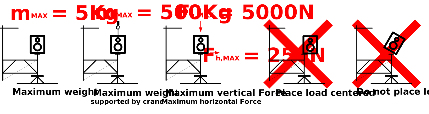
Center of gravity of the DUT must be at the center of the platform.
The maximum turning moment (e.g., by placing the DUT off centered) induced to the platform must be smaller than 250 Nm when DUT is placed on platform
Do not exceed the maximum lateral (horizontal) force of 250 N induced to the platform when DUT is positioned on platform
Do not exceed the maximum vertical force of 5000 N induced to the platform when DUT is positioned on platform
Do not exceed the maximum allowed load of:
5 kg with proper mounting on platform.
500 kg if supported by a crane.
For measurement and placement of objects above a weight of 5 kg a crane must be used. The operator is responsible to make sure, a crane is available for this purpose.
English: Regular Safety Checks#
Regular safety checks must be done every 100 hours of operation, at least every 3 months. The safety check or any service of the device must be done by skilled personnel. Personnel must well understand the exact instructions given in the assembly instructions. Through their qualification they must be familiar with risks mentioned in the instructions and avoid any danger in a thoughtful manner.
The regular check includes:
Check that the area of movement of the Near Field Scanner is clearly marked as area, restricted to authorized personnel only.
Check all screw connections and refasten if necessary. Pay particular attention to:
screws for floor mounting.
all screws attached to the floor profiles.
all screws attached to the diagonal cross stays between floor profile and center table foot.
all screws on the bottom side of the table, connecting the center table foot.
Check the whole device for any obvious damage.
Check the function of the Emergency stop.
Exchange Power switch box (Emergency Stop) after 20 Years of use.
German: Anweisungen für die Bedienung#
Der Betreiber hat dafür zu sorgen, dass die Bedienung des Nahfeld-Scanners nur von geschultem, technisch ausgebildetem Personal durchgeführt wird.
Die Personen müssen die Bedienungsanleitungen („R&D System User’s Guide Near Field Scanner“ und „Near Field Scanner Hardware Setup Guide“) und diese Sicherheitsbestimmungen gelesen und verstanden haben und verantwortungsvoll die Bestimmungen beachten.
KLIPPEL übernimmt keine Haftung für Schäden oder Verletzungen verursacht durch die Nichtbeachtung der Sicherheitsbestimmungen oder Instruktionen der Bedienungsanleitungen.
Automatischer Betrieb#
Der Bewegungsbereich des Nahfeld-Scanners muss klar als gesperrter Bereich gekennzeichnet sein, so dass eindeutig erkennbar ist, dass das Betreten nur geschultem und befugtem Personal erlaubt ist.
Stellen Sie sicher, dass sich keine Personen im gesperrten Bereich befinden, wenn das Gerät läuft, egal ob es sich um den automatischen Betrieb oder um manuelles Bewegen handelt.
Stellen Sie sicher, dass keine Personen den gesperrten Bereich betreten, während das Gerät läuft.
Stellen Sie sicher, dass sich die Power Switch Box/Emergency Stop immer in Reichweite des Bedieners befindet, wenn der Nahfeld-Scanner läuft.
Allgemein#
Gefahr Quetschen/Stolpern/Verletzen: Benutzen Sie den Nahfeld-Scanner in einem speziellen Raum oder bauen Sie einen Zaun um die Maschine, so dass keine unbefugten Personen in den Bewegungsbereich kommen können.
Gefahr Stolpern: Stellen Sie sicher, dass beim Einrichten, Prüfen und Betreiben des Nahfeld-Scanners ausreichende Beleuchtung vorhanden ist (mindestens 300 lx)
Bringen Sie Warnhinweise an, wenn das Betreiben des getesteten Lautsprechers zu gefährlichen Zuständen führen kann, (zum Beispiel sehr starke elektromagnetische Abstrahlung, stark erhöhte Schall Abstrahlung, hohe elektrische Spannung)
Gefahr hoher Schalldruck: Stellen Sie sicher, dass der Nahfeld-Scanner in einem separaten Raum arbeitet, so dass an anderen Arbeitsplätzen die Schallabstrahlung von 80dB nicht überschritten wird.
Die Bediener müssen bei hohem Schalldruck (über 80 dB SPL) jederzeit Schallschutz für die Ohren tragen.
Durch KLIPPEL nicht zertifizierter Umbau/Modifizierung des Nahfeld-Scanners ist nicht erlaubt. Benutzen Sie nur originale, von KLIPPEL gelieferte Teile, wie Kabel, Netzteil und alle anderen Teile. Reparaturen und Veränderungen sind nur durch KLIPPEL Personal oder genau nach Anweisungen von KLIPPEL durchzuführen.
Stellen Sie sicher, dass die Anlage ordnungsgemäß auf dem Fußboden montiert ist, bevor schwere Messobjekte auf den Messtisch platziert werden.
Stellen Sie sicher, dass die Stromzufuhr des Nahfeld Scanners ordnungsgemäß gegenüber Überlastung abgesichert ist.
Alle Personen, die den Nahfeld-Scanner betreiben, müssen regelmäßig informiert werden über die Gefahren beim Betreiben, unter anderem:
Quetschgefahr: Halten Sie Sicherheitsabstand, wenn sich die Achsen bewegen. Es kann zu Verletzungen kommen, wenn Körperteile in dem Bewegungsbereich der Maschine kommen.
Stolpergefahr: Gehen Sie vorsichtig in der Nähe der sich bewegenden Maschine und beachten Sie die Beschaffenheit des Bodens. Stolpern kann zu Verletzungen führen.
Platzieren der Messobjekte auf dem Nahfeld Scanner#
Stellen Sie die Messobjekte (Lautsprecher, Boxen und anderes) sicher auf den Messtisch, verhindern Sie das Herunterfallen durch geeignete Maßnahmen.
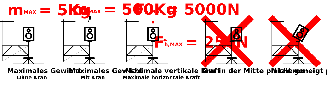
Das Zentrum der Schwerkraft des Messobjekts muss in der Mitte des Messtischs liegen.
Das maximale Drehmoment das auf den Messtisch einwirkt, muss kleiner als 250 Nm sein.
Die seitliche Kraft (horizontal) die auf den Messtisch einwirkt, darf 250 N nicht überschreiten.
Die vertikale Kraft, die auf den Messtisch einwirkt, darf 5000 N nicht überschreiten.
Stellen Sie sicher, dass die maximale Last nicht überschritten wird, von:
5 kg bei guter Befestigung auf dem Messtisch
500 kg mit Befestigung durch einen Kran
Für Messobjekte über 5 kg muss für das Platzieren und Halten während der Messung auf dem Nahfeld-Scanner Messtisch ein Kran verwendet werden. Stellen Sie sicher, dass ein Kran zur Verfügung steht.
German: Regelmäßige Sicherheitskontrollen#
Nach jeweils 100 Stunden Betrieb muss eine Sicherheitskontrolle durchgeführt werden, aber mindestens aller 3 Monate. Die Sicherheitskontrolle und alle Servicearbeiten müssen von geschultem Personal durchgeführt werden. Diese Personen müssen die Instruktionen in der Aufbauanleitung exakt verstanden haben und beachten. Sie müssen entsprechend qualifiziert sein, um die, in den Instruktionen genannten Risiken zu kennen und in umsichtiger Weise zu verhindern.
Die regelmäßigen Sicherheitskontrollen enthalten:
Prüfen, dass der Bewegungsbereich des Nahfeld-Scanners klar markiert ist und für unautorisierte Personen verboten.
Alle Schraubverbindungen des Nahfeld-Scanners prüfen und bei Bedarf nachziehen. Besondere Aufmerksamkeit bei folgenden Verbindungen:
Schrauben zur Bodenbefestigung
Schrauben an den Bodenprofilstangen
Schrauben an den diagonalen Kreuzen zwischen Bodenprofilstangen und Center Table Fuß
Schrauben an der Bodenseite des Center Tables, die den Fuß verbinden
Den gesamten Aufbau nach sichtbaren Fehlern oder Schäden absuchen.
Die Funktionstüchtigkeit des Notfall-Stopp-Schalters (Emergency Stop) prüfen
Die Strom-Schalt-Box (Power Switch Box/Emergency Stop) soll spätestens nach 20 Jahre Gebrauch erneuert werden.
NFS - Tutorial#
Part 1 - Viewing NFS Results#
What is the goal of this tutorial?#
The tutorial presents the complete NFS processing of an example measurement. It is focused on the following key aspects:
Give an overview of the database structure and the NFS modules
Getting familiar with Parameter and Results of the NFS Field Identification
Get to know the NFS Visualization Software
Measurement Database#
Example data used in this manual is stored in the Web Example database. If not downloaded already, get it from the latest R&D release <https://www.klippel.de/go/current-rnd-release> and open the web-based database.
See also
View Results for general information on how to download this database, open and view results in dB-Lab.
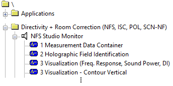
Select in the folder Directivity + Room Correction the driver object NFS Studio Monitor.
Measurement Data Container#
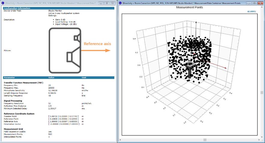
Select the operation 1 Measurement Data Container.
This operation stores all relevant measurement information for the further holographic identification. Open the Summary window to see all information. The 2nd window Measurement Points shows the distribution of the measurement grid, as well as the reference system that specifies the position of the DUT.
Field Identification#
Select the Operation 2 Holographic Field Identification and open the Property Page.
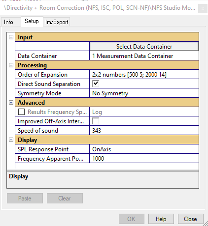
Have a look at the following parameters:
Order of expansion: -defines the number of expansion terms.
Direct Sound Separation - If checked, Field Separation is active and room reflections are compensated
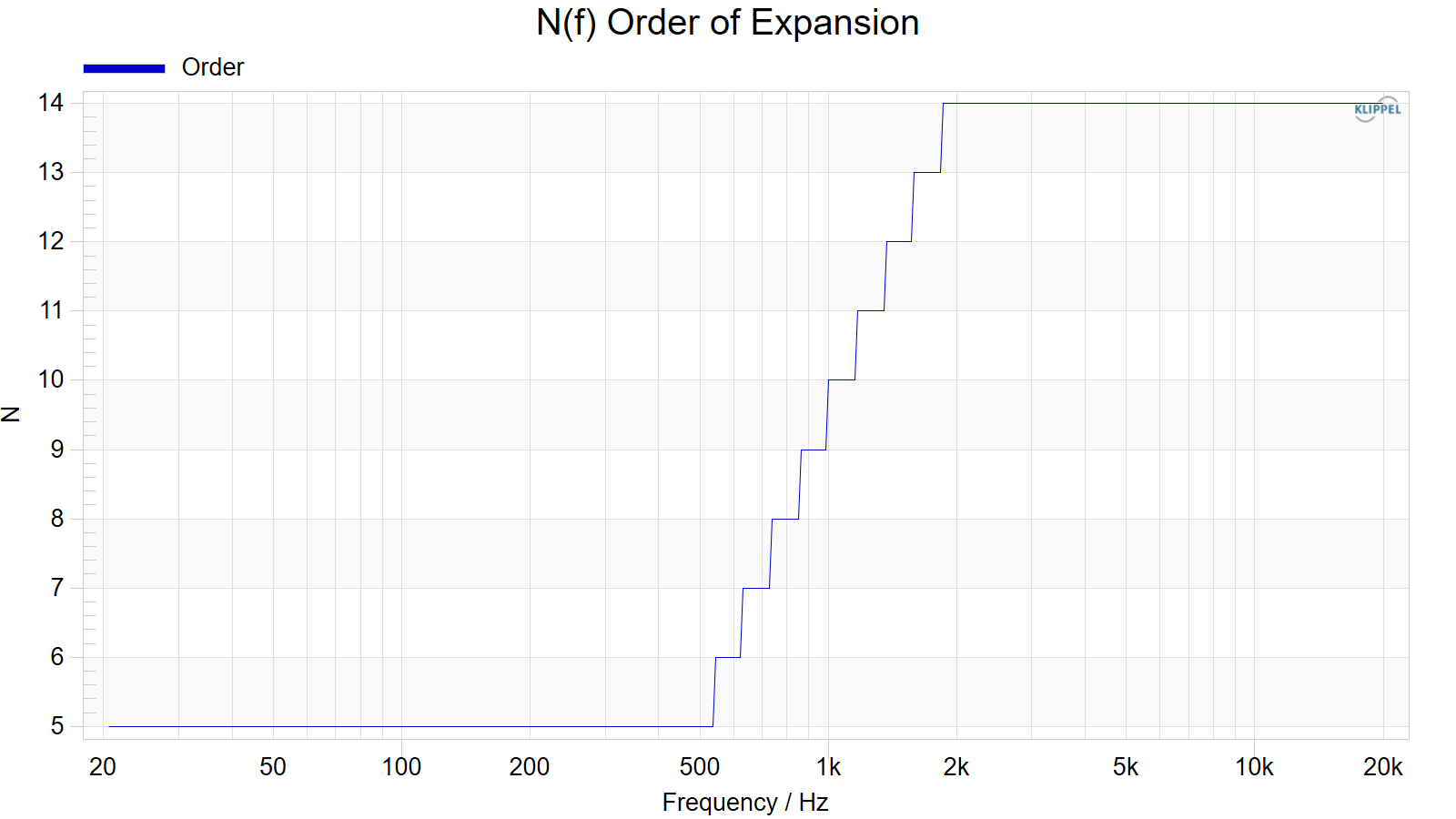
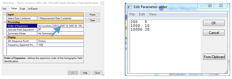
In the example, the order is defined dynamically over frequency. The left column defines the frequencies and the right column the order of expansion. As seen in the edit field for f < 500 Hz the order is set N = 5. For higher frequencies the order is increased up to N = 14 for f > 2kHz.
Order:
//Freq. in Hz     Order
     500            5
    2000           14
Fitting Error#
Open the Fitting Error window. The E(f) Fitting Error is an indicator for the accuracy of parameter identification.
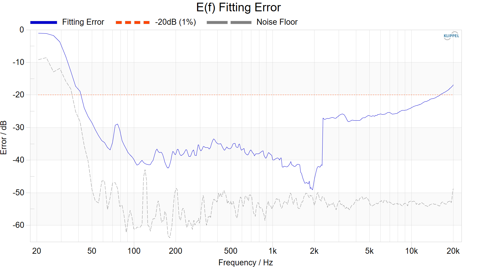
As seen in the picture the fitting error is below the threshold of -20 dB (1 % error) over a large frequency band. For low frequencies (f< 500 Hz) the high error is caused by noise and is uncritical. Also, above 16 kHz the fitting error rises but it is still below -15 dB, which is sufficient for this frequency range. (For further information see Fitting Error)
Frequency Response#
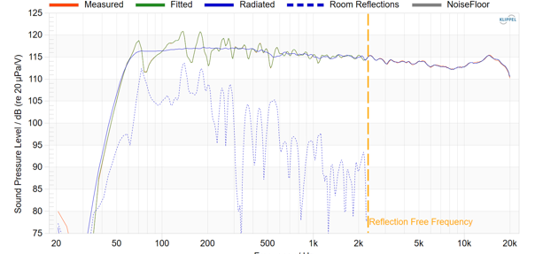
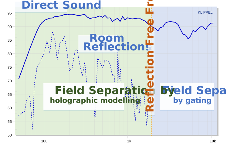
Open the Frequency Response window. The graph shows the response of a point at the measurement surface in the near field of the device. For low frequencies the room reflections are detected by the holographic approach and the direct sound of the loudspeaker is identified. For frequencies above the Reflection Free Frequency the reflections are cut out using time windowing.
NFS Visualization#
Once the Field identification is done, the data can be analyzed using NFS Visualization operations. This operation can extrapolate the sound pressure based on the coefficients of the spherical wave expansion and generate far field characteristics, near field visualization as well as data for further analysis with external software like MATLAB, Python etc.
Select the Operation 3 Visualization (Freq. Response, Sound Power, DI) and open the Property Page.
Input Data#
To link the result data of the Field Identification module the operation with the source data is selected.
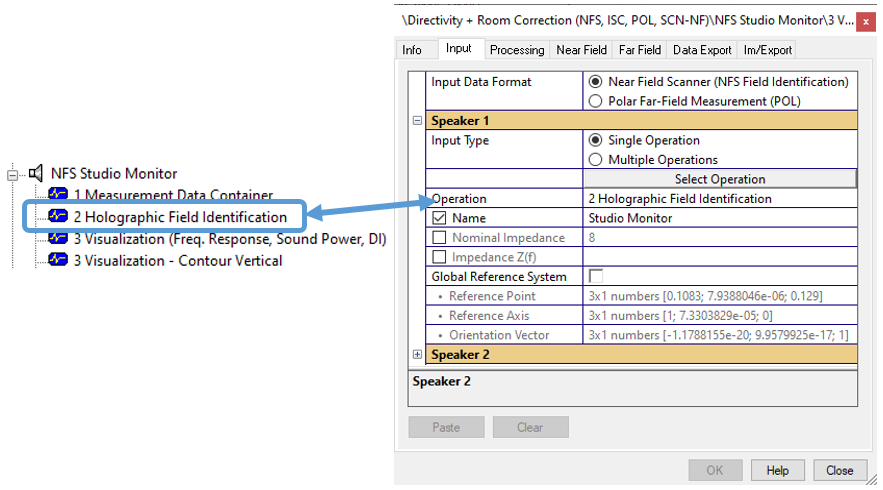
In addition, the Input page has other optional settings like a manual definition of the Reference Coordinate System in order to adjust small mismatches in the positioning of the device under test.
Far Field Characteristics#
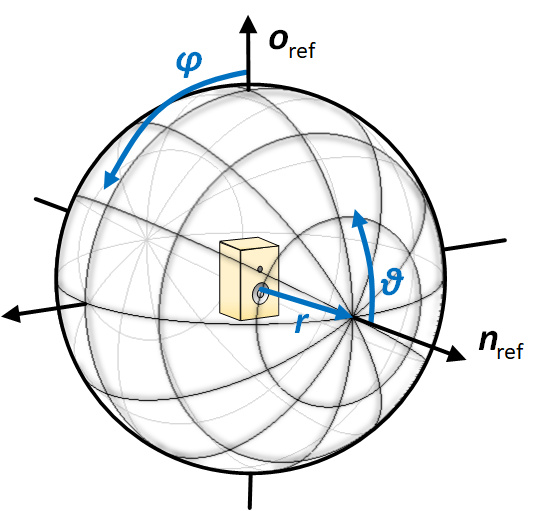
For a lot of applications acoustical measurements of loudspeakers are performed in the far field. In order to have a simple relation between distance and the sound pressure level (1/r law). Also, the directivity of loudspeaker is usually analyzed under far field conditions. In the far field the radiation pattern is independent from the distance, the sound power constant and the 3D sound radiation can be reduced using a spherical surface with the two radiation angles theta and phi.
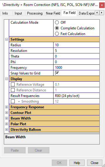
Select the Far Field tab of the Property Page. The Far Field Property Page has three section:
- Settings:
This section specifies the spherical surface that is used for the analysis by Radius and angular Resolution.
In addition, the angles Phi and Theta can be defined freely to select a specific listening point (e.g. On-Axis) or orientation of the Contour Plot (e.g. vertical or horizontal).
Also, the Frequency can be defined for the Polar Plot and the Directivity Balloon.
- Display:
This section includes standard post processing that is applied to all graphs like linear scaling to a Reference Voltage or Reference Distance (using the 1/r law) or Smoothing over the frequency band.
- Settings of the graphs:
The other categories are containing specific settings for the individual graph windows. (For more details refer to the Reference.)
Interactive Analysis#
Change the Parameter angles Phi and Theta to following values:
Phi = -90°
Theta = 30°
This modification does immediately update the graphs.
The Contour Plot and the Polar plot is changed to Phi= -90° which corresponds to the horizontal plots.
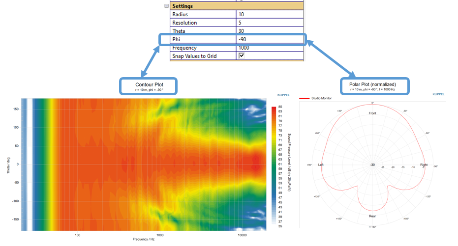
The selected phi angle is shown in the subtitle of the result window.
Select the H(f) Magnitude + Phase response and the derived measures (Impulse Response, Group Delay). The data is shown for the selected Theta and Phi angle.
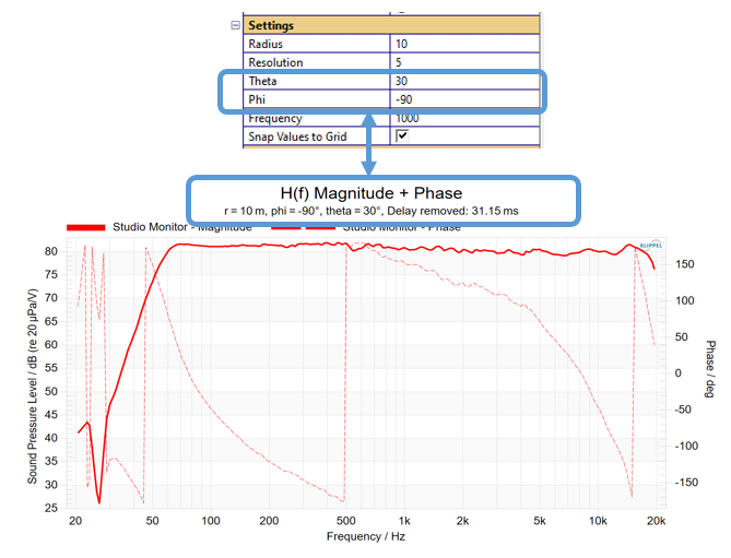
The selected Point is shown in the subtitle of the result window.
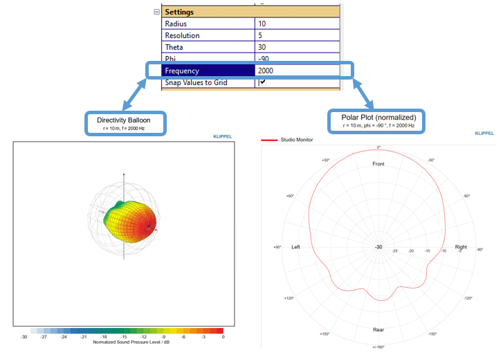
Change the Frequency to 2 kHz. This will update the Directivity Balloon as well as the Polar Plot.
Display - Scaling and Processing#
Similar to the coordinate and frequency selection, some standard processing can be applied to the results interactively. For example, these features can be used to generate a Sensitivity curve for your data sheet.
Example - Sensitivity:#
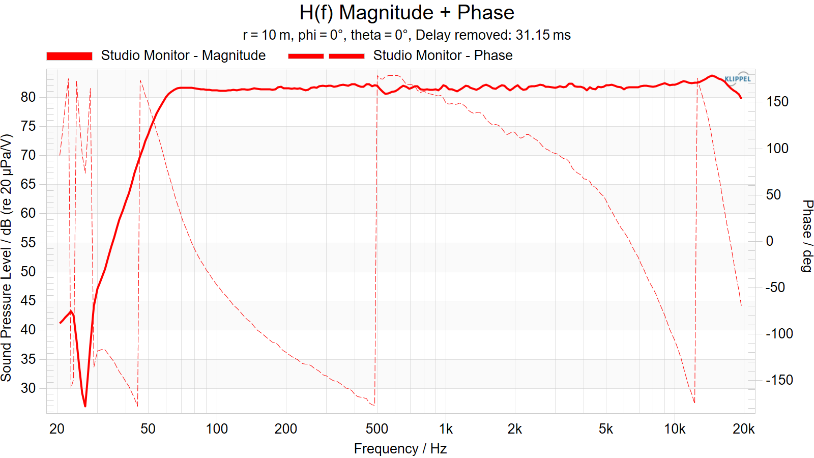
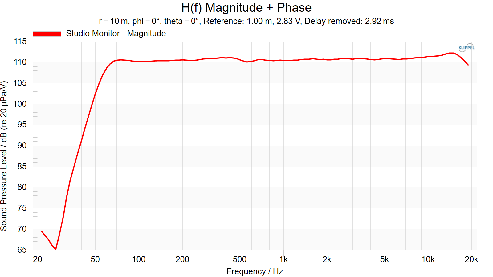
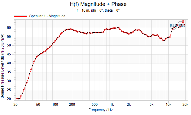
Open the graph Frequency Response and set the Phi and Theta back to 0°. As seen in the subtitle of the graph, the window is showing frequency response at 10 m On-Axis.
Note
In general, all graph of the Visualization are referred to 1Vrms.
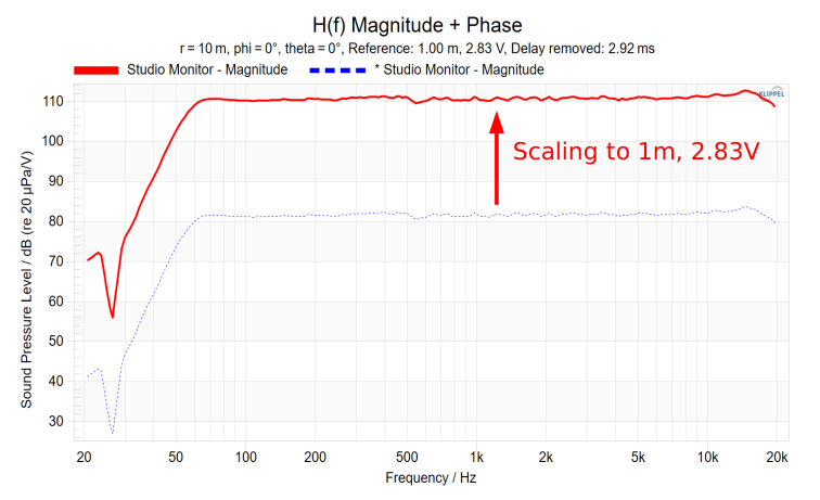
To determine from this 10m far field response the Sensitivity, the data has to be scaled, which can be done using the Reference Distance and Reference Voltage Parameter.
Set the Reference Voltage to 2.83 V (1W for 8 Ω) and the Reference Distance to 1 m. Both parameters will scale the Magnitude. The Reference Distance will also influence the Phase Response by removing a time delay using the 1/r law.
Furthermore, the Sensitivity curve can be smoothed and interpolated to a desired frequency resolution. For example, set the Smoothing to 3 points per octave and select the R40 (12 pts/oct) ISO frequencies.
Note
The category Frequency Response is providing further display options for the graph. E.g. different option for the Phase visualization (unwrapping or remove of time delay)
Directional Characteristics versus Frequency#
The way how a loudspeaker emits sound can change a lot with frequency. At low frequencies, most loudspeaker behave like point sources with an omnidirectional radiation pattern. And for high frequencies, the sound is radiated more focused into a specific direction. Using loudspeaker systems with more than one transducer, the sound field is also influenced by constructive and destructive interference (e.g. in the frequency range of the crossover) or can even be actively controlled using line arrays or planar arrays and digital signal processing. To understand these complex properties the Visualization is providing a set of common graphs.
Sound Power + Directivity Index#
Sound Power and Directivity Index give very comprehensive information about the sound field. The Sound Power is describing the total energy that is emmited by the loudspeaker. The Directivity Index describes the ratio between the sound pressure level On-Axis to the mean sound pressure level in all directions. These two measures help to understand, how much a loudspeaker is beaming and how the relation between direct sound and reverberant sound would be.
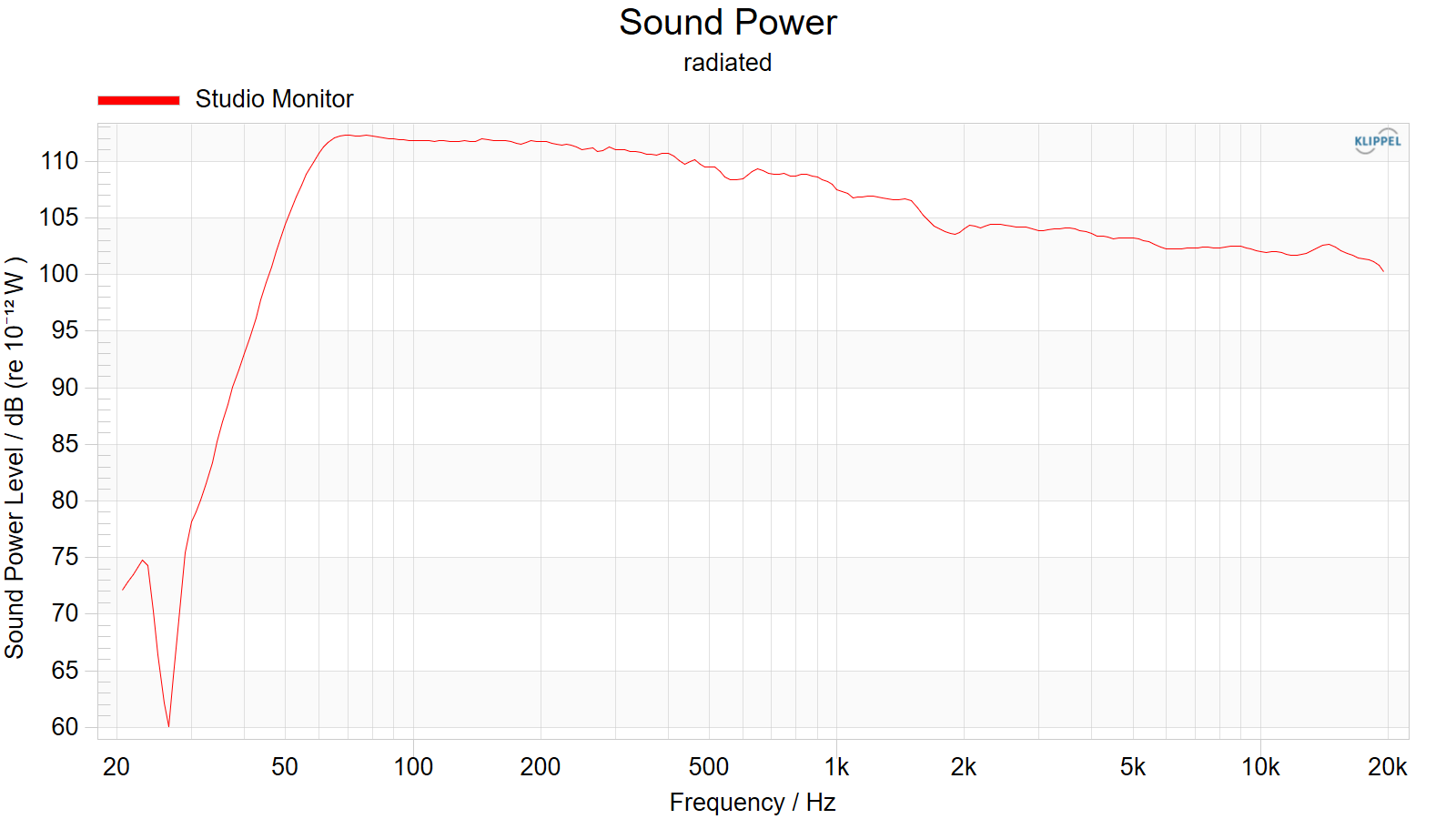
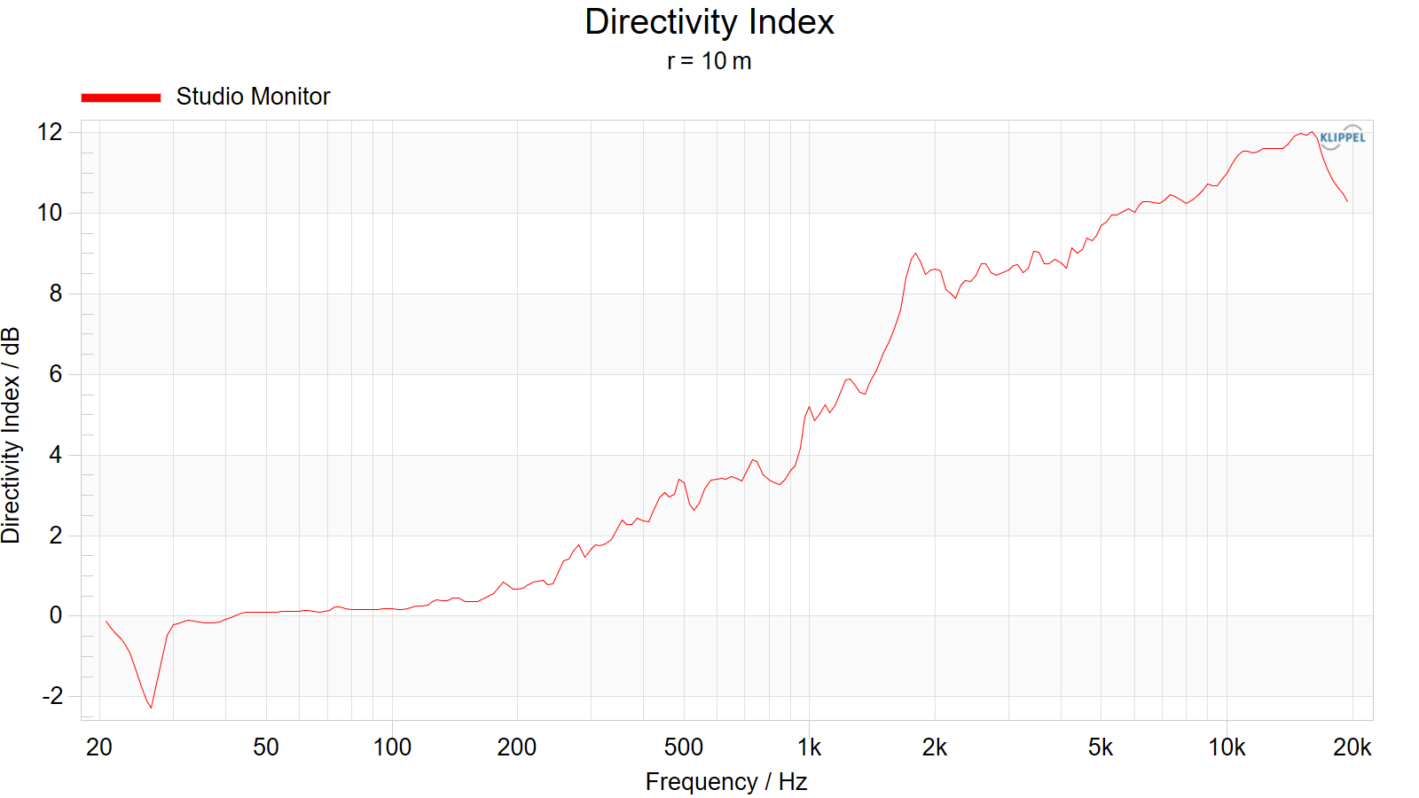
For this example speaker the directivity is 0dB below 100Hz, which is typical for an omnidirectional sound field. Increasing the frequency also the directivity index increases, which shows that the loudspeaker is beaming to the front.
Contour Plot + Beamwidth#
Understanding the frequency dependent behavoir of the device under test the Contour plot is very useful. For a defined phi angle (φ =0° vertical/ φ =90° horizontal) this graph visualizes the sound pressure level versus frequency and the polar angle theta.
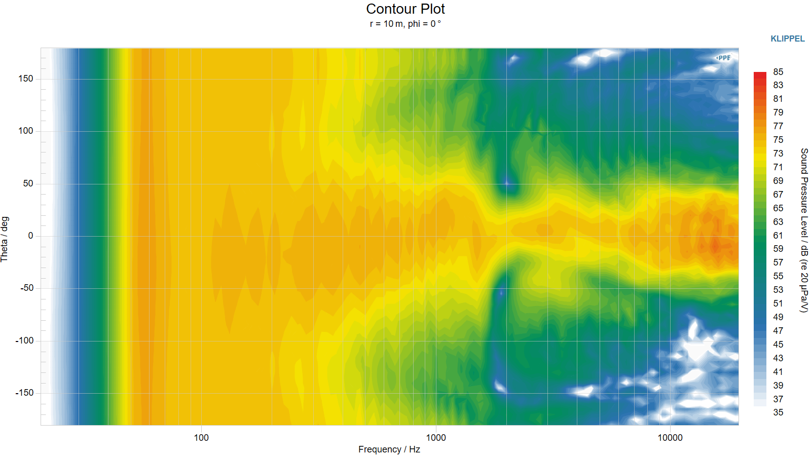
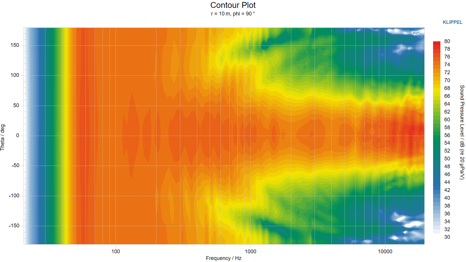
Thus the Contour Plot can show very clear at which frequencies and which positions side lobes or cancelations appear. This is very helpful when validating for example a crossover configuration, a mechanical design of a waveguide or complex DSP-Setup for beam steering or beam shaping.
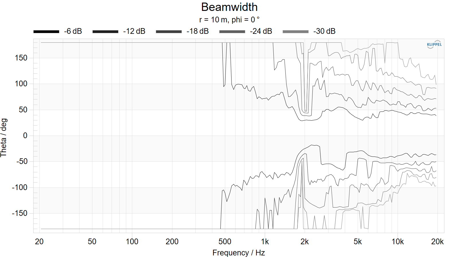
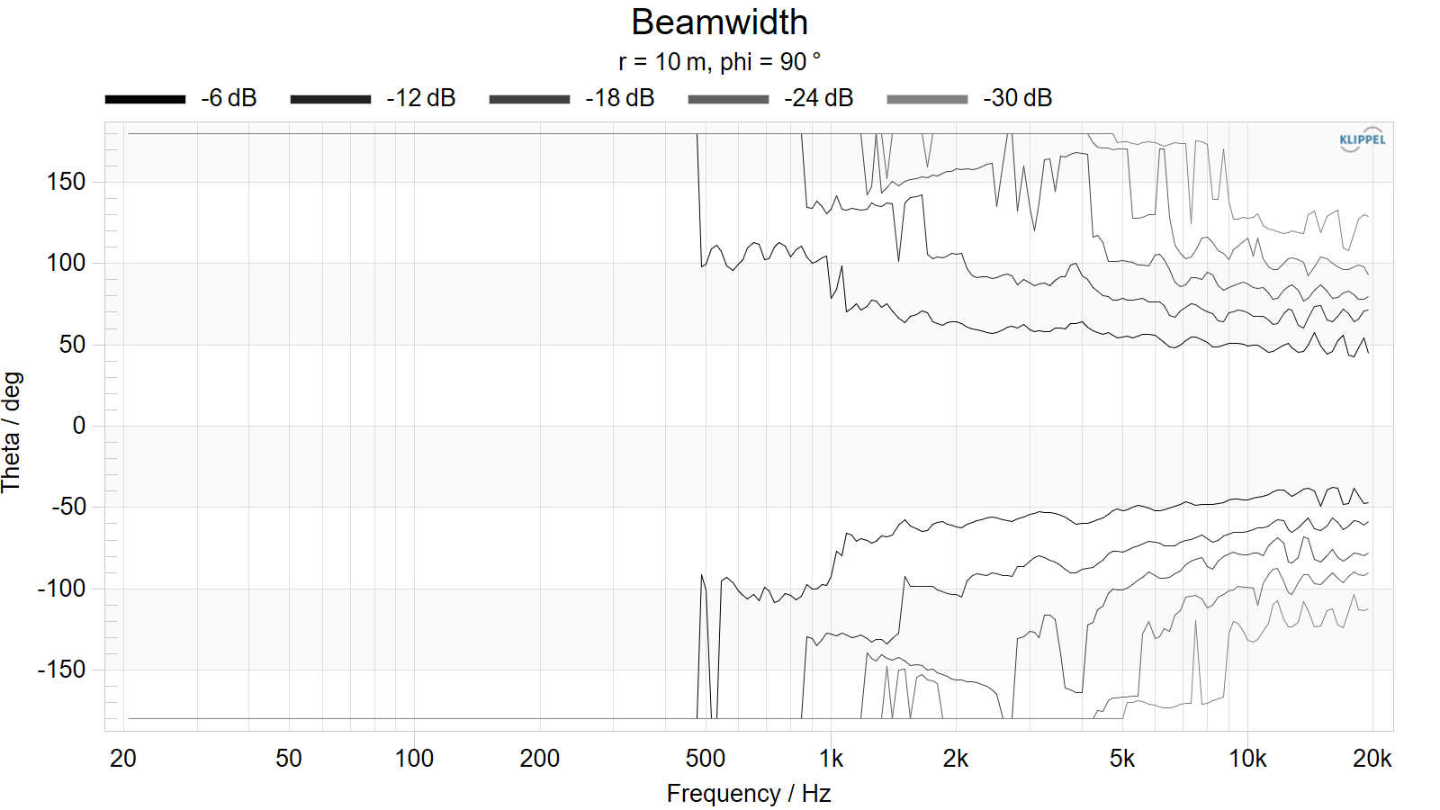
To define the coverage of speaker according to IEC60268-21, the Beamwidth plot is showing at which angle the sound pressure level has dropped by a certain level. This example speaker has a horizontal coverage angle of about ± 50°.
Note
To customize the Contour Plot there are a couple of display option in the corresponding category of the Property Page.
Polar Plot + Directivity Balloon#
The sound field of specific frequencies (e.g. at a mechanical resonances of the cone) can be investigated further with the Polar Plot and the Directivity Balloon.
The Polar visualizes the radiation pattern over the Polar angle theta for a defined Phi angle (φ =0° vertical/ φ =90° horizontal) and the Directivity Balloon illutrate the directivity in all directions over both theta and phi.
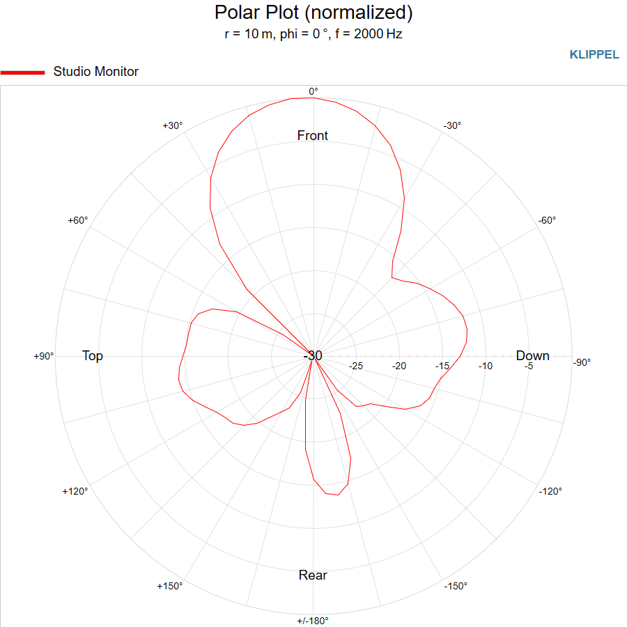
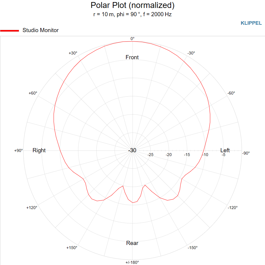
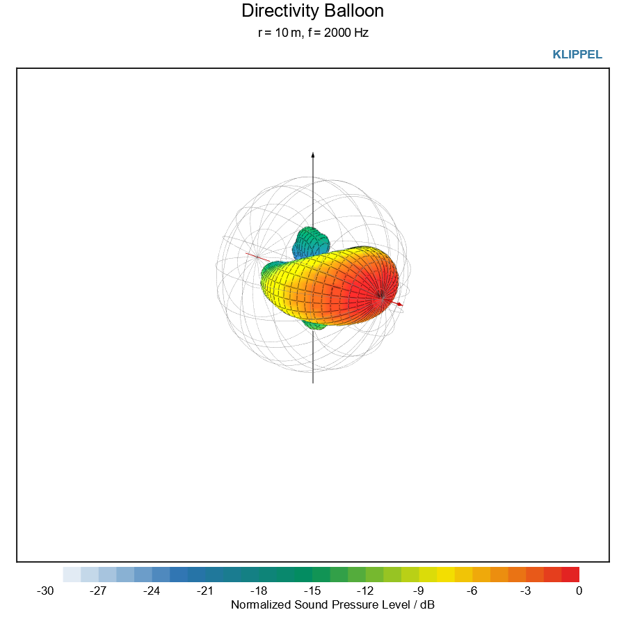
Both graphs have several display options, which can be found in the corresponding category of the Property Page.
Note
Polar Plots of multiple frequencies can be easily overlaid in the same result window using copy and paste.
Near Field Analysis#
There are a lot of audio application (laptops, smart phones, tablets, near field monitors, etc.) which have their target listening area in the near field.
In difference to the far field in this region of the sound field is very complex. Sound pressure and particle velocity are out of phase and the 1/r law cannot be used.
However, the Near Field Scanner measurement system accurately models, characterizes these near field effects and can extrapolate the sound pressure level at any point that is outside the scanning surface.
To understand this almost infinite amount of possible data the NFS Visualization has a special Near Field Analysis module that helps analyzing the area around the device.
Near Field - Sound Pressure Distribution
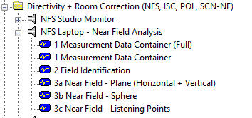
Select the Driver Object NFS Laptop – Near Field Analysis and open the Operation 3a Near Field Plane and 3b Near Field Sphere.
As shown in these examples the sound pressure level around the audio device is visualized. The projection surfaces can be scaled and positioned freely in 3D space to analyze the user defined listening area.
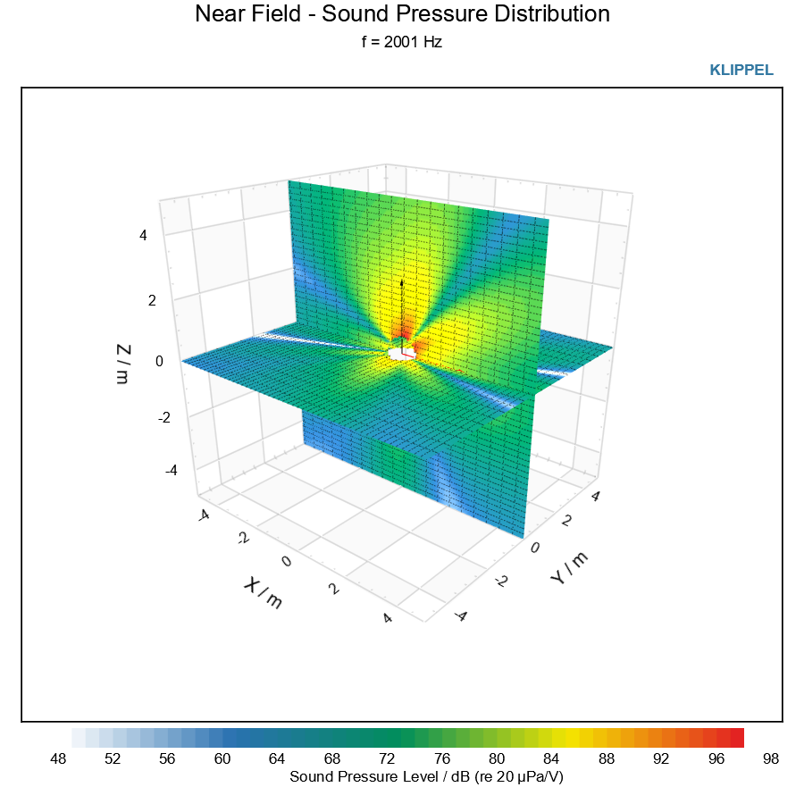
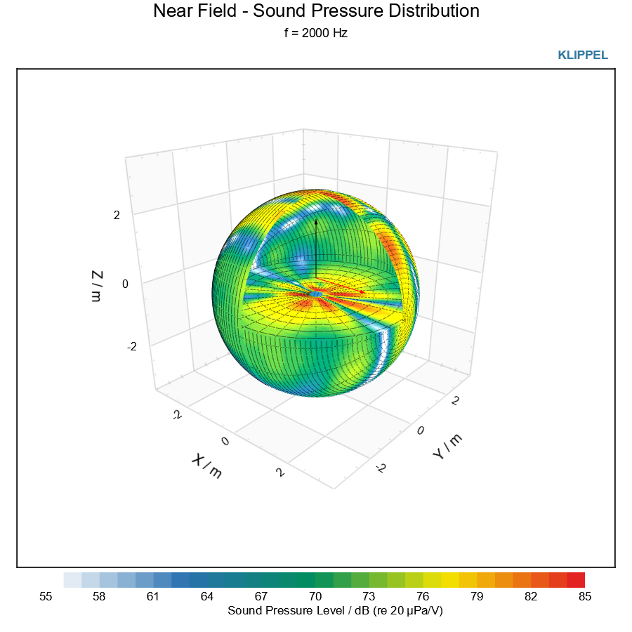
In addition to the magnitude, the holographic model is also providing accurate phase information, which can be visualized as well.
Near Field – Listening Points
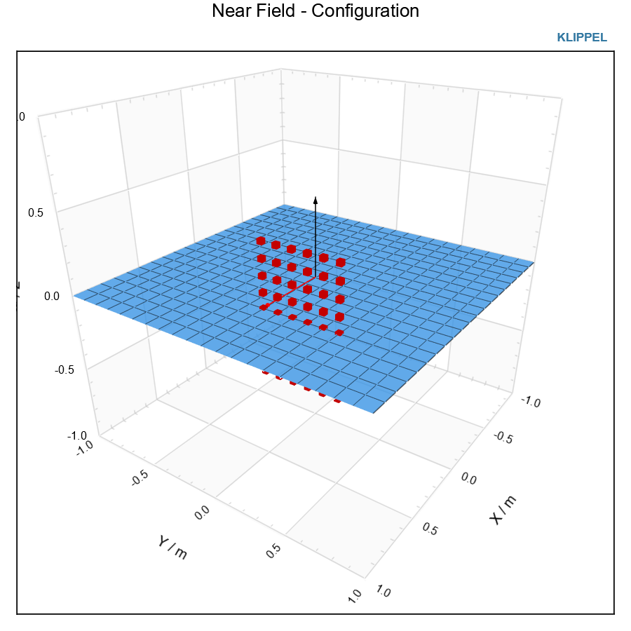
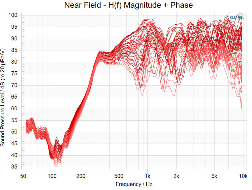
In order to analyze the frequency behavior in the near field, Listening points can be defined freely in the near field by a list of coordinates.
At these Listening points, the Near Field Analysis module calculates transfer function in magnitude and phase.
In addition, the position of the points is visualized in the Near Field – Configuration windows.
Note
Similar to the far field characteristic, also the near field analysis is providing standard processing function e.g. smoothing
Part 2: Perform a Measurement#
What is the goal of this Tutorial?#
The Tutorial Part 2 is a guide for the execution of a NFS measurement. It is focused on the following key aspects:
Get to know the measurement software and measurement hardware
Performing a NFS measurement
Analyze the results of a NFS measurement
Optimize Field Identification configuration and validate the results
Quick Setup Guide#
In addition to tutorial part 2, there is a Quick Setup Guide that summarizes the most important steps to setup a measurement. Use this pdf for printing. If the Robotics software is installed the Quick Setup Guide can be found on the website: Quick Setup Guides.
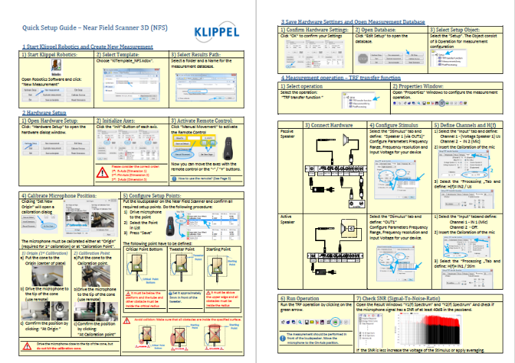
The following chapters describe all steps of the guide more in detail.
Start Robotics and Create New Measurement#
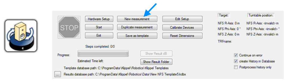
Open the Klippel Robotics Software and click the Button “New Measurement” to select a template database.
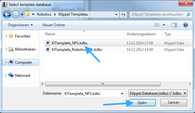
Open the folder: C:/ProgramData/Klippel/Robotics/Klippel Templates/NFS
Select the file: KlTemplate_NFS.kdbx and press Open
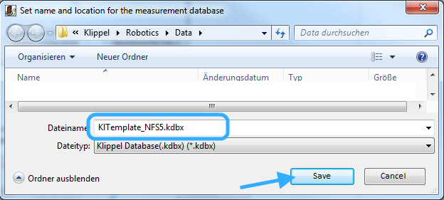
Now select a result path. The results of your measurement are saved in this folder. Define a name of the measurement database and press Save.
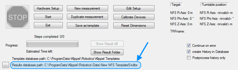
After selecting, the path of the Result Database is displayed in the left bottom corner.
Initialize Near Field Scanner Hardware#
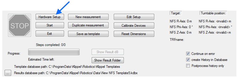
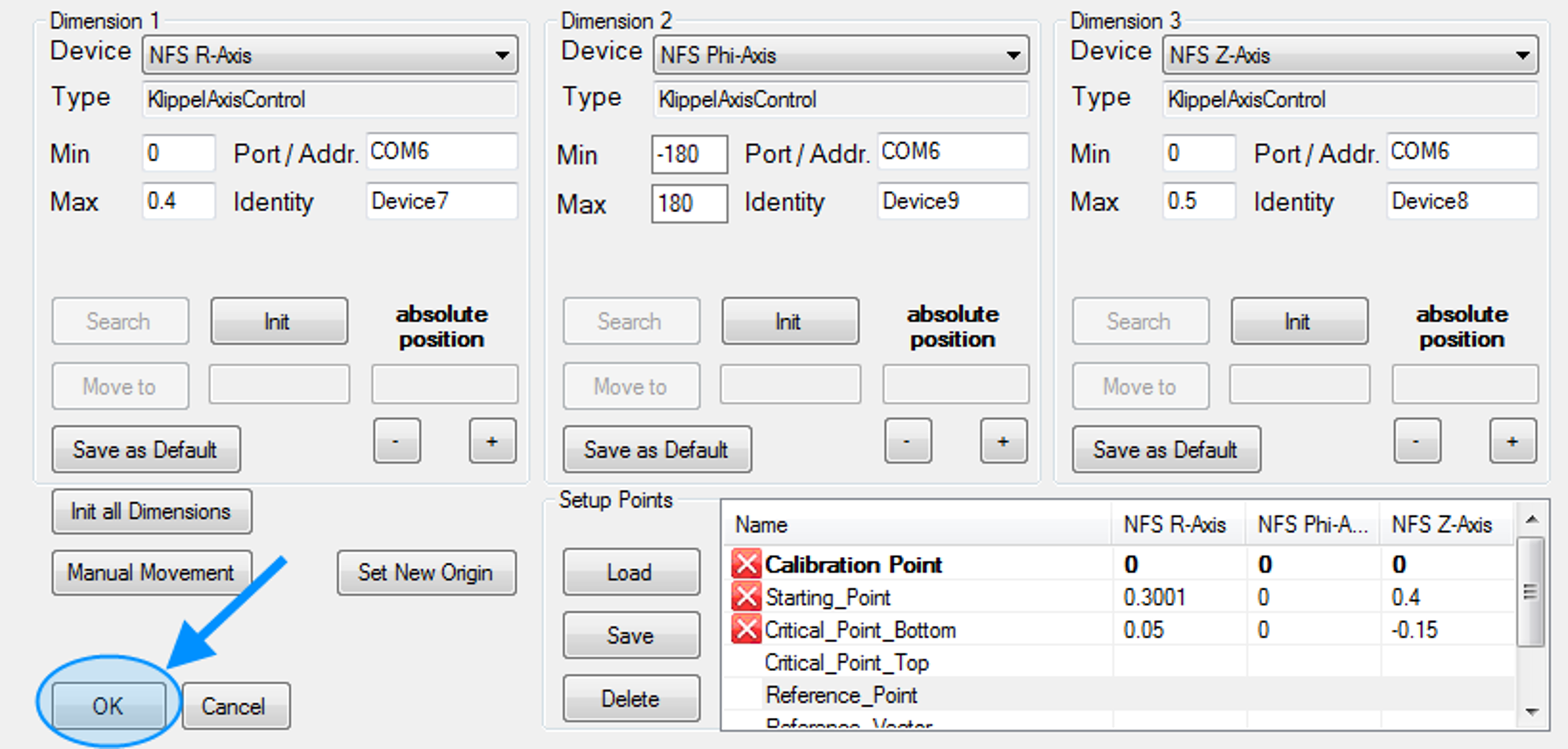
Open the Hardware Setup.
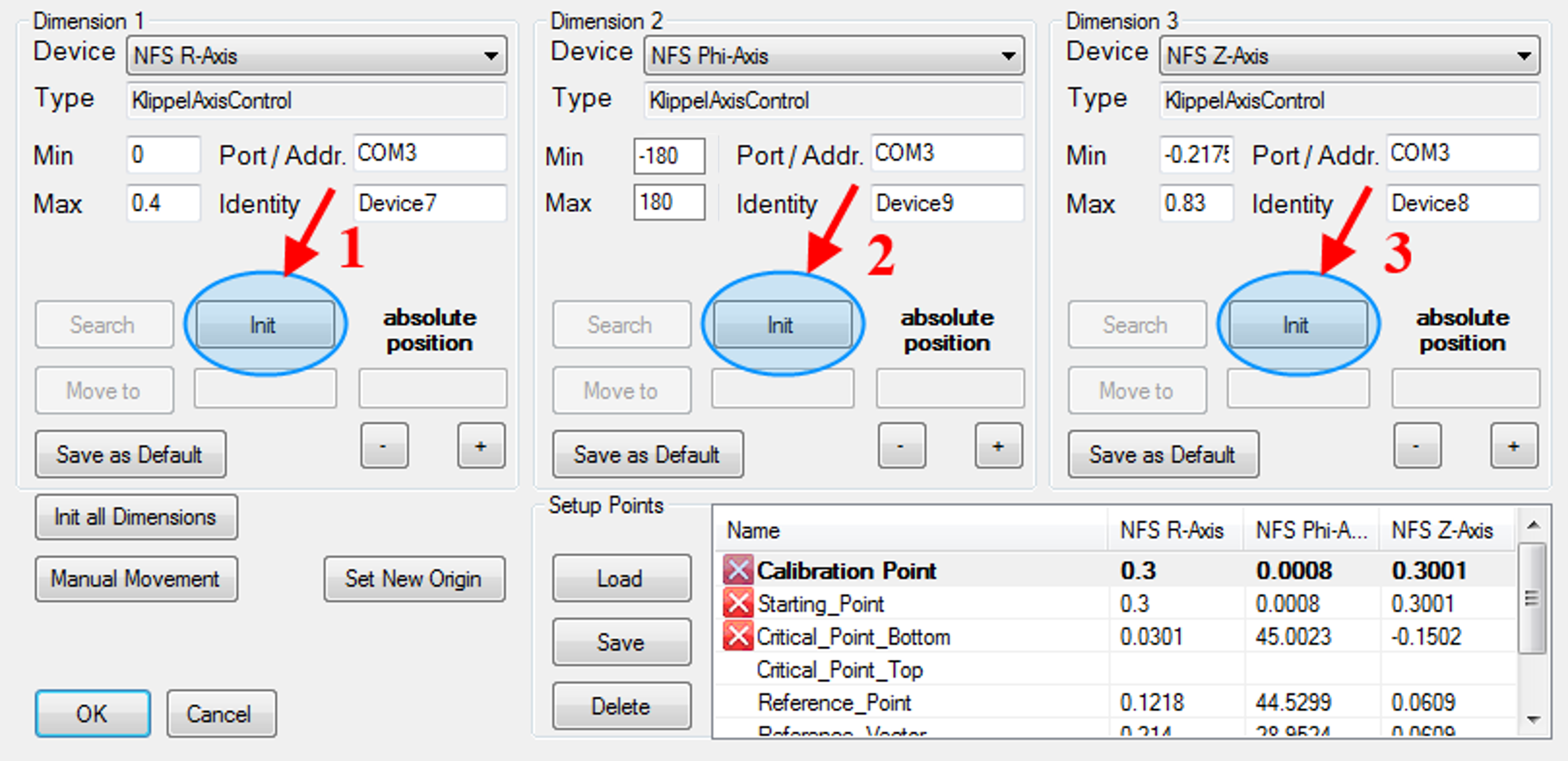
Check if the devices are assigned correctly.
- Dimension 1: NFS R-Axis
Port/Addr.: COM<Portnumber>
- Dimension 2: NFS Phi-Axis
Port/Addr.: COM<Portnumber>
- Dimension 3: NFS Z-Axis
Port/Addr.: COM<Portnumber>

Also make sure, the correct COM-port is set for operation of the Near Field Scanner Hardware. Please check the Windows Device Manager, which COM-Port has been assigned to the USB-RS485 converter.
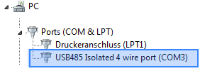
Use this port number and enter it in the Port/Addr field (e.g. for COM port 3 enter “COM3” into the Port/Addr field).
Start the Initialization of each axis by clicking on the “Init” - Buttons.
Warning
Initialize the Dimensions, starting with the R-axis (Dimension 1), continuing with Phi-Axis (Dimension 2) and Z-Axis (Dimension 3).
The following behavior of the NFS Hardware is expected:
R-Axis moves outwards and stops at the end switch
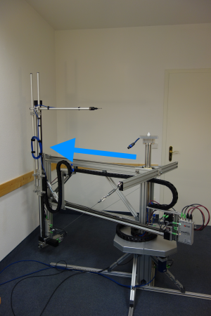
Phi-Axis moves counterclock wise to the phi end switch and then it moves ack to phi=0° position
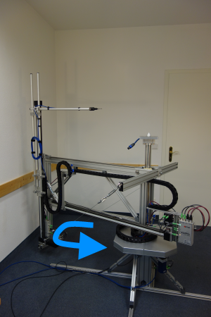
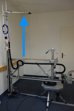
Z-Axis moves upwards up to the end switch
Activate Manual Movement#
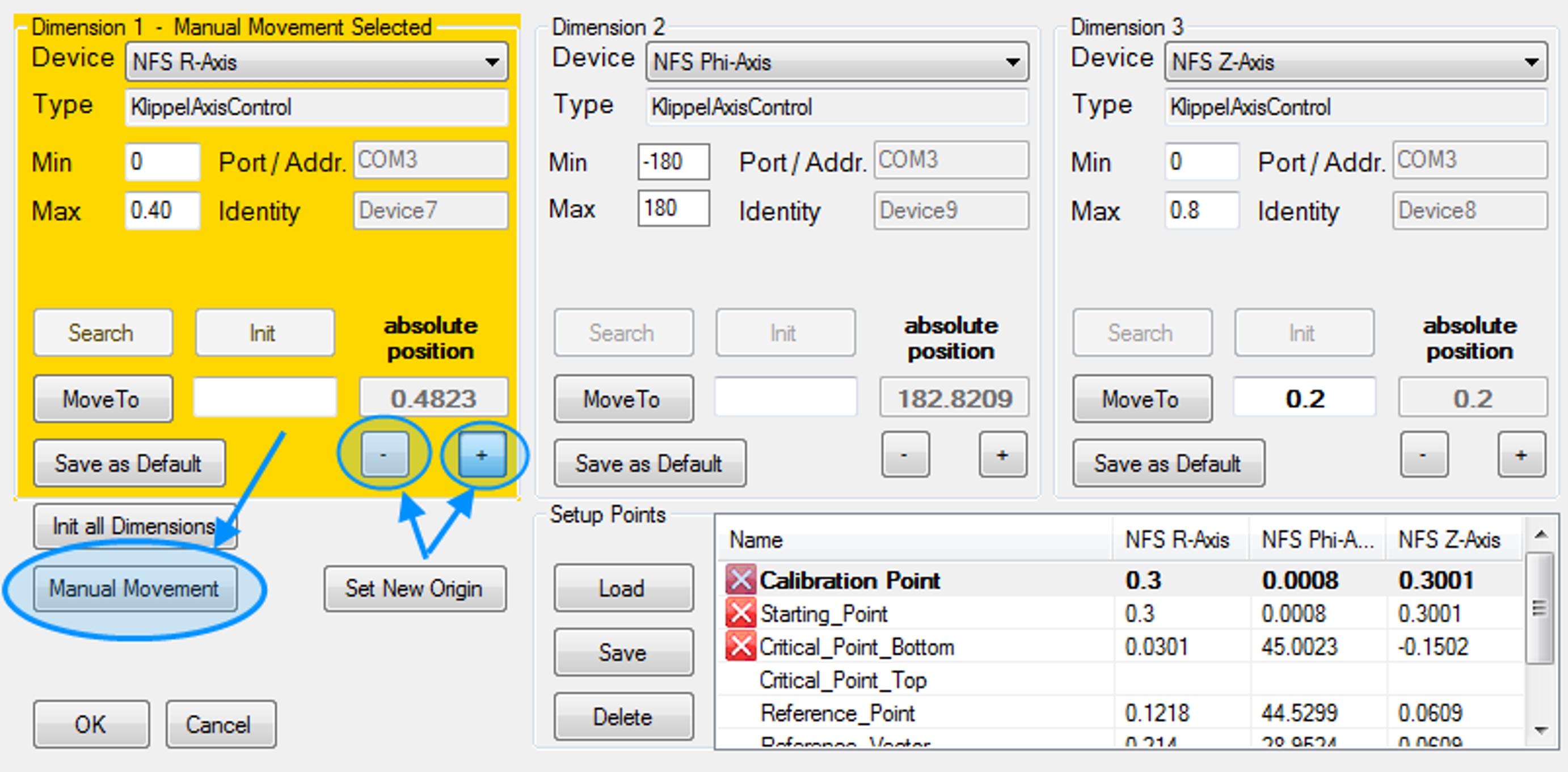
Activate the “Manual Movement” mode (see the following picture). Now use the Remote Control or the ‘-’and ’+’ buttons to move the microphone.
Remote Control - Movement Modes#
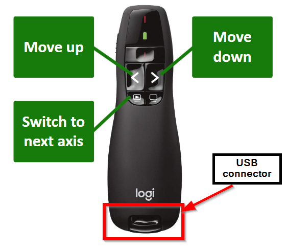
The remote control has a USB connector at the bottom, simply pull it out and plug it into your PC’s USB port, and it will be ready to use.
- Continuous Movement - Rough Positioning
Dragging a movement button, the axis accelerates at first and continues with a uniform speed. Lifting the button stops the motion.
- Single Step Mode – Precise Positioning
Pressing shortly a movement button, the axis will move a single step.
Calibrate Microphone Position#
For the first measurement and after mechanical adjustments the microphone must be calibrated at both:
the Origin position and
Calibration Point.
For further measurement:
the calibration at the Calibration Point is sufficient
You can skip the calibration at the Origin
Calibrate Microphone at Origin#
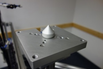
The Origin is defined at the center of the Near Field Scanner Hardware on the top surface of speaker plate and can be calibrated using the calibration cone. Put the cone at the center of the speaker plate.
Warning
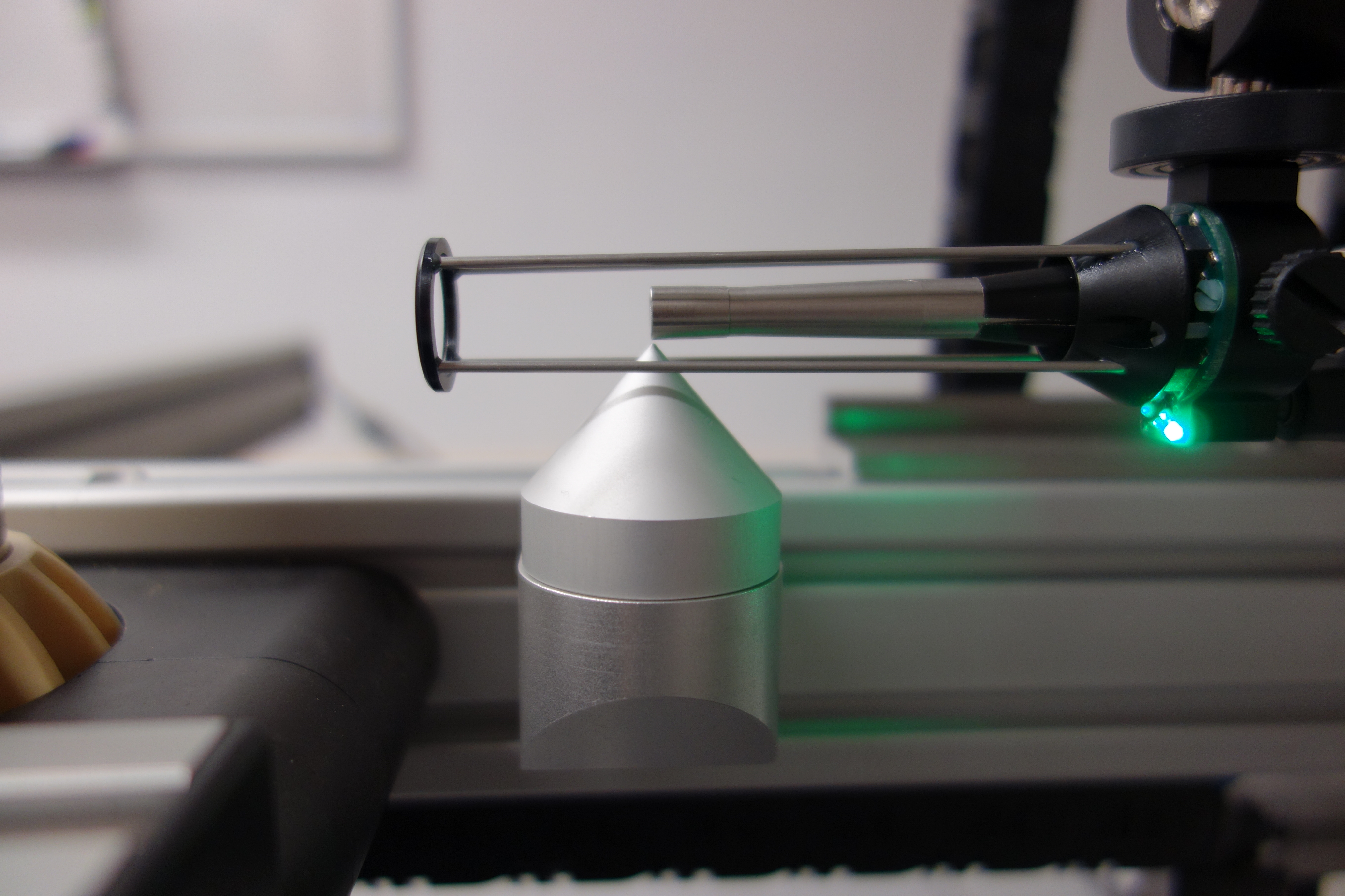
Drive the microphone close to the tip of the cone, but do not hit the calibration cone.
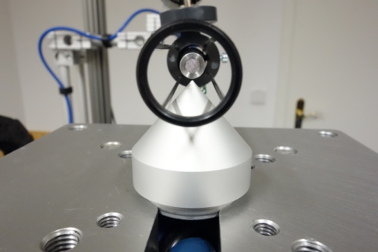
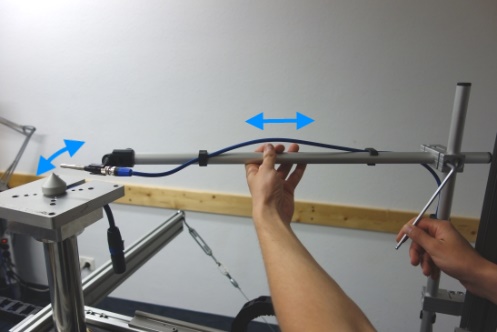
If the microphone cannot be positioned to the origin point by moving the axis, adjust the microphone position by hand to reach this point.
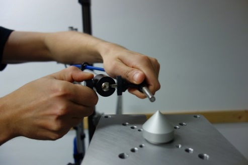
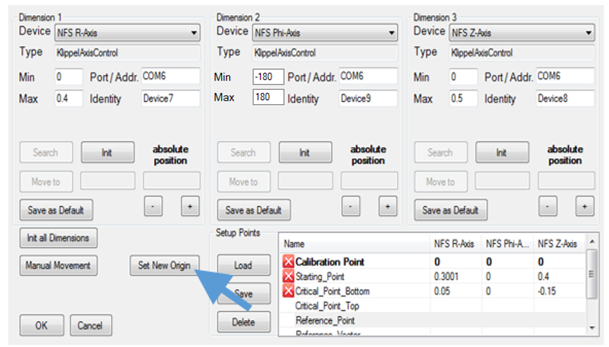
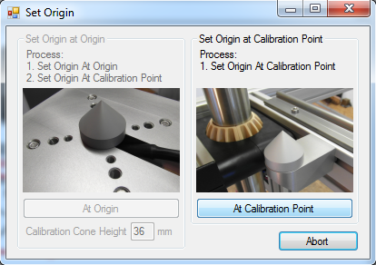
After the microphone is centered to the Origin, press Set New Origin and select At Origin.
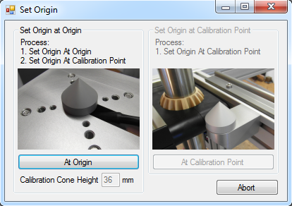
When setting the origin, the height of the calibration of 36 mm will be considered automatically. The Z=0 position will be exactly on the top surface of the speaker plate.
Calibrate Microphone at Calibration point#
To avoid the need of setting the Origin every time the system is used, save a second point to the system, which is used as calibration point in subsequent measurements.
Put the calibration cone on the calibration point on the arm of the Near Field Scanner.
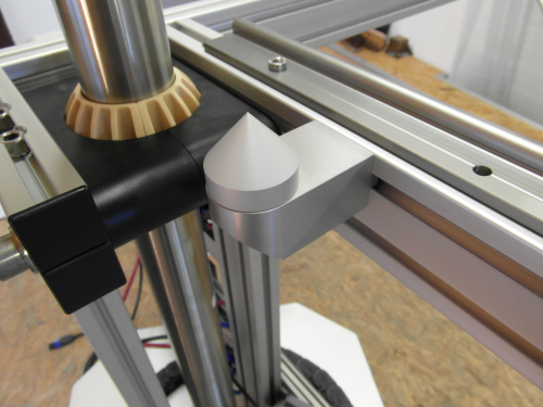
Now use the remote control to drive microphone to the tip of the calibration cone.
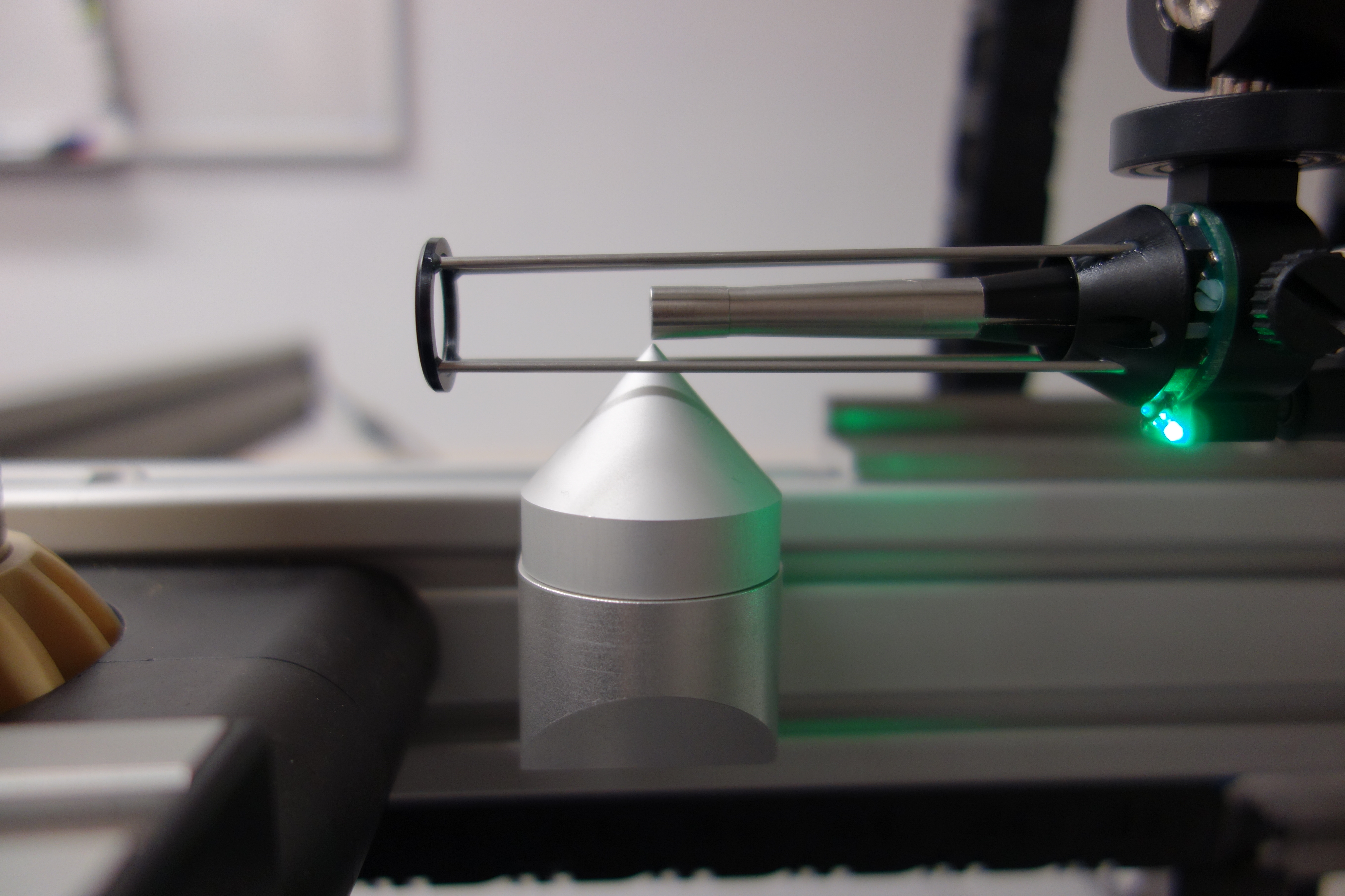
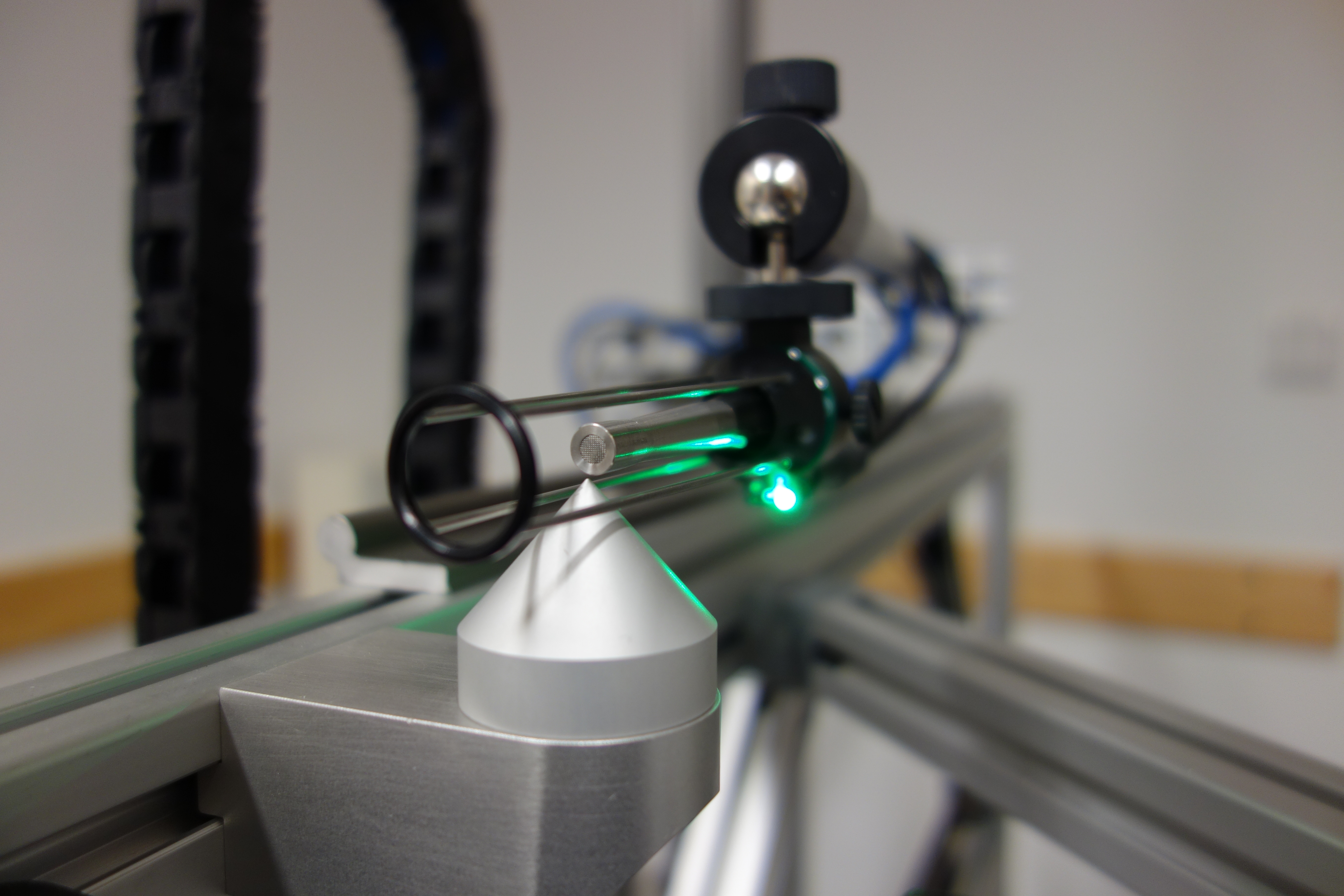
Warning
Drive the microphone close to the tip of the cone, but do not hit the calibration cone.
After the microphone is centered to calibration cone select At Calibration Point.
Set Axes Limits#
Z-Axis#
Use the Remote Control or the + button to drive the Z=Axis upwards to the maximum end switch. Once it arrive the end position the movement will stop and the MAX LED on the Z-Axis Control Box is turned on.
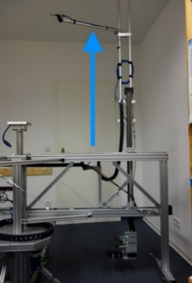
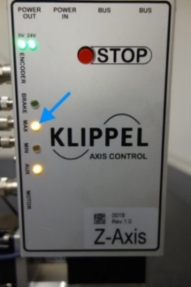
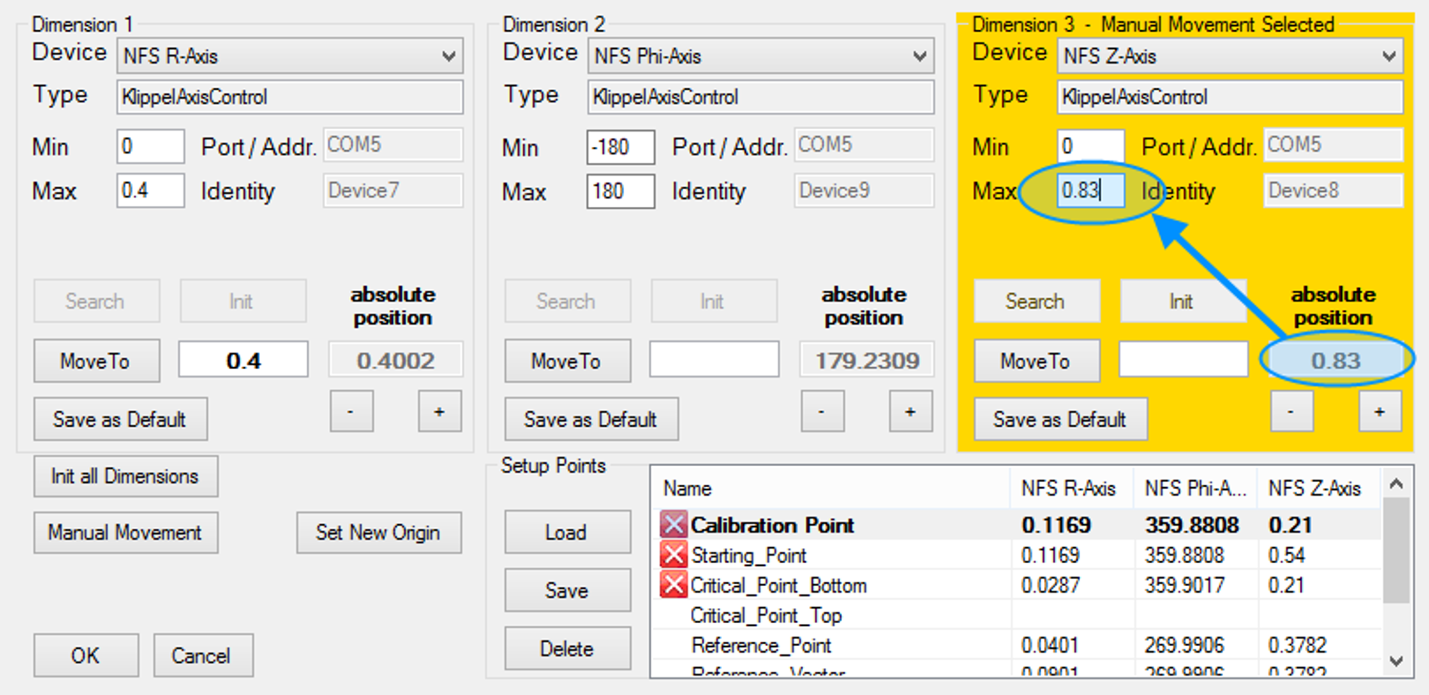
Move the Z-Axis a bit downward until the MAX LED will turn off. Read the absolute position of the Z-Axis in the hardware setup and set the max value of the Z-axis to the current position.
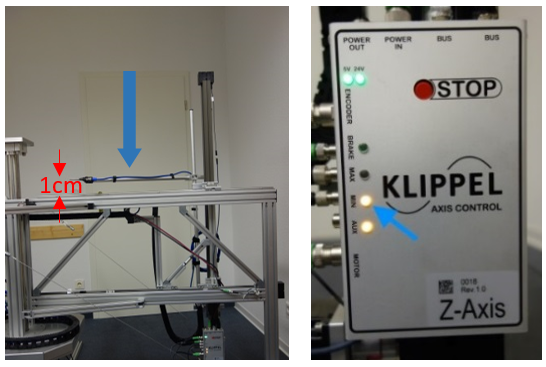
Continue with the minimum z value. Use the remote control or press the ‑ button to drive the Z-Axis downwards into the minimum end switch.
Warning
Take care, that the microphone pole will not hit an obstacle. If necessary move r-Axis outwards.
Once it arrive the end position the movement will stop and the MIN LED on the Z-Axis Control Box is turned on.
The minimum z-position is supposed to be below the speaker platform. It should be about 1 cm above the frame structure. If not please adjust the microphone pole by hand and repeat the calibration at the Origin.
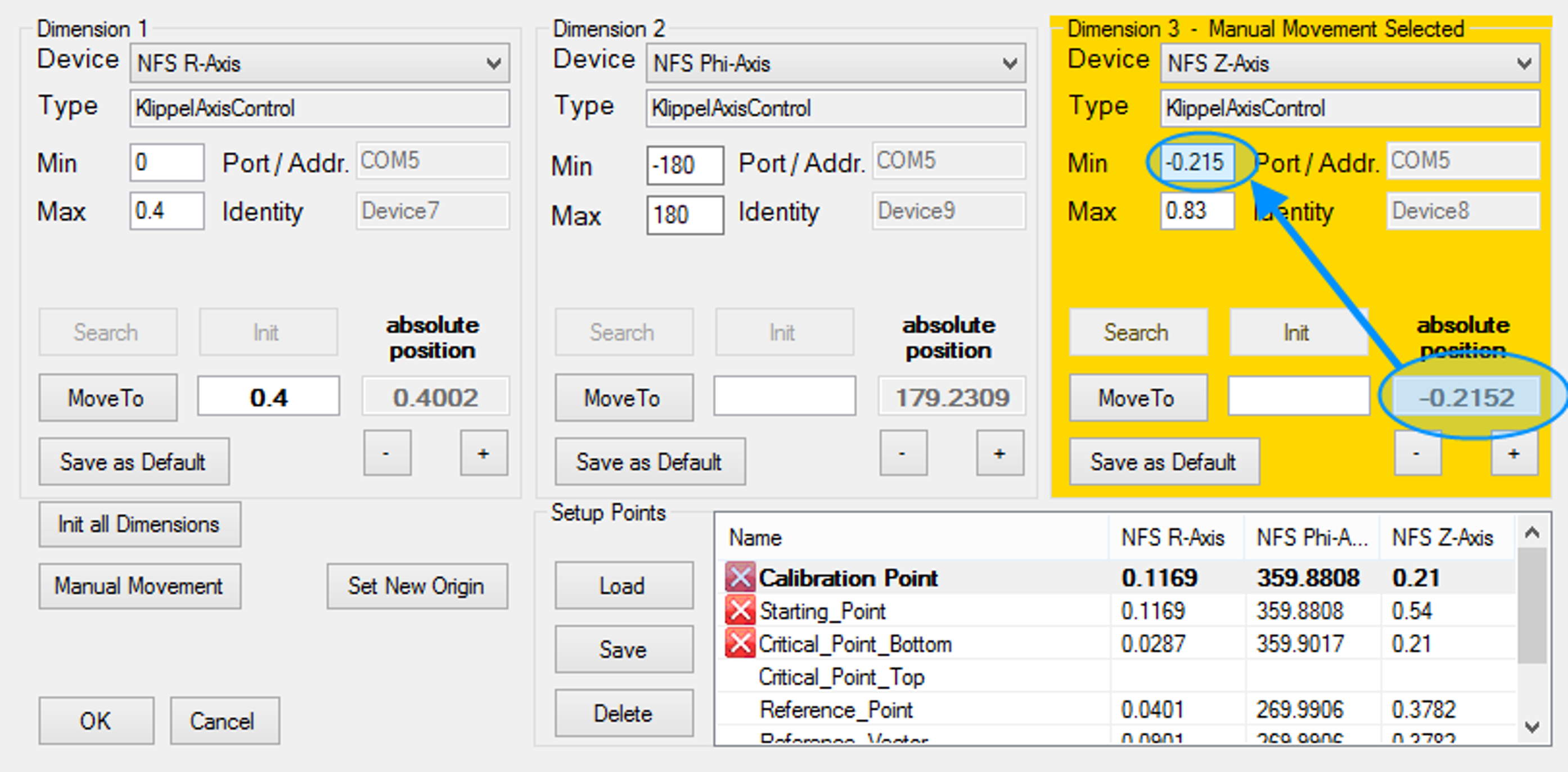
Move the Z-Axis upward until the MIN LED will turn off. Read the absolute position of the Z-Axis in the hardware setup and set the min value of the Z-axis to the current position.
Repeat the same procedure for the R-Axis.
Specify the Dimensions of the Device#
Remove the calibration cone and put the device on the NFS hardware. Connect the cable with the device as well.
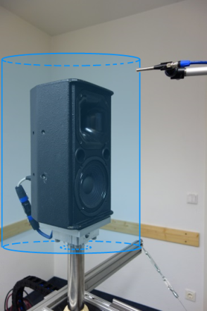
The NFS measurement is performing a scanning on a complete cylindrical surface around the device under test (DUT). The size of the cylinder is defined by setting specific points.
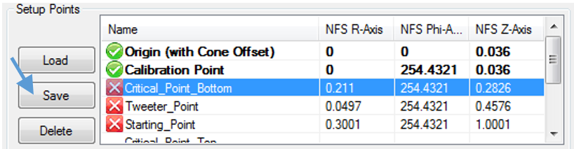
All points are shown in the table in the hardware setup. The points are distinguished between required and optional points. The required points are marked at the beginning with a cross. It is necessary driving the microphone to each of the required points before starting the measurement. After setting a required point the mark will change into a check.

Setup Points#
To define the size of the measurement surface, two points are required. These are the critical point bottom and the starting point. The points are defining the minimum cylinder of the measurement grid. Inside the cylinder, the microphone cannot be positioned.
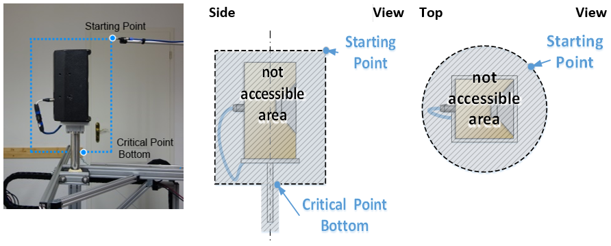
Critical Point Bottom#
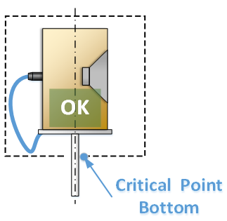
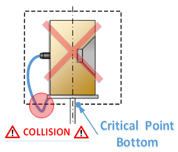
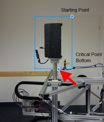
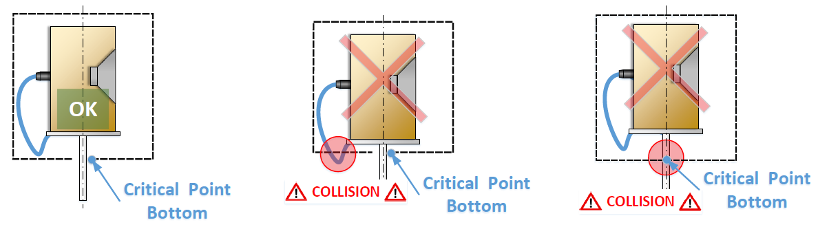
Critical Point Bottom is defining the height of the cylinders lower surface and the minimum radius at the bottom surface, which can be reached from the microphone without hitting any obstacle. See the following examples:
- Good Configuration
- Critical Point Bottom is correctly defined.
- Wrong Configuration
- Z-Position of Critical Point Bottom is too high. The microphone will hit the cable.
- Wrong Configuration
- R-Position of Critical Point Bottom is too small. The microphone will hit the stand.
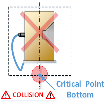
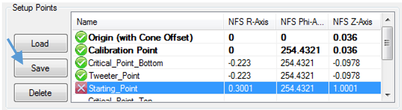
Drive the microphone to the critical point bottom. Select the Critical_Point_Bottom in the Setup Points table and press Save. Now the current microphone position is saved in the table and the cross changes into a check.
Tweeter Point#
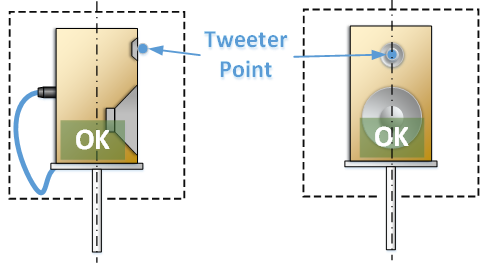
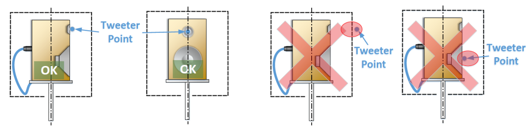
The Tweeter point defines the origin of the holographic field identification. It is recommended to set it about 5 mm in centered in front of the speaker. For a system with multiple speakers, set it in front of the tweeter, which is close to the acoustic center for high frequencies.
- Good Configuration
- The Tweeter Point is approximately 5mm in front of the Tweeter.
- Wrong Configuration
- Tweeter Point is in front of the woofer. This requires a very high order of expansion to identify the sound field.
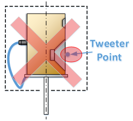
- Wrong Configuration
- The tweeter point is outside the scanning surface.
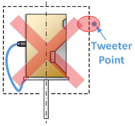
Starting Point#
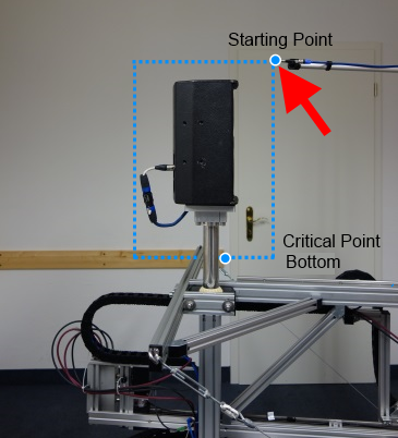
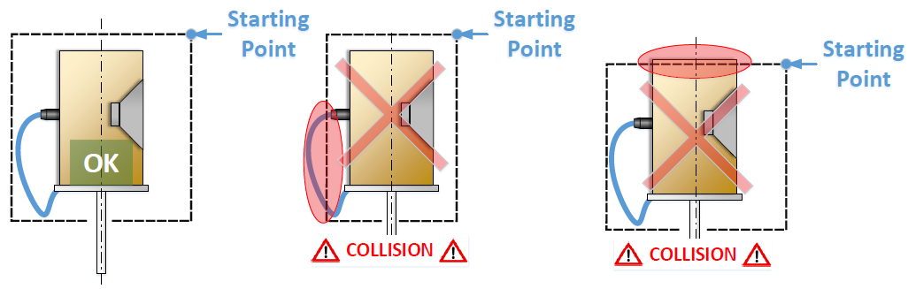
The Starting Point defines the upper limit of the cylinder. Make sure that all obstacles and cables are inside the cylinder. Otherwise, the microphone can hit it during the measurement. It is recommended to have a safety distance between microphone and the device of about 5-10 cm and not set the starting point as close as possible.
- Good Configuration
- Starting Point is correctly defined.
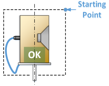
- Wrong Configuration
- Z-Position of Starting Point is too low. The microphone will hit the DUT.
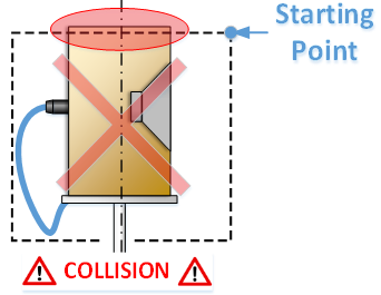
- Wrong Configuration
- R-Position of Starting Point is too small. The microphone will hit the cables.
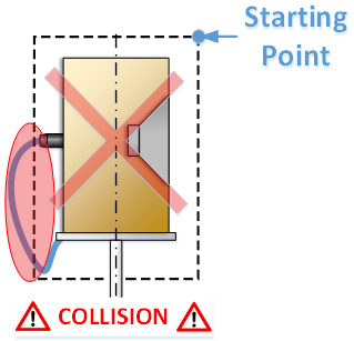
Drive the microphone to the Starting Point. Select the Starting_Point in the Setup Points table. And press save to confirm your settings.
Critical Point Top (for hanging setup only)#
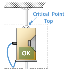
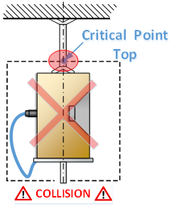
The Critical Point Top is an optional parameter and is just required for a hanging device, which is mounted for example in the ceiling. For this special application, there is critical area on the top surface, which cannot be reached by the microphone.
- Good Configuration
Critical Point Top is correctly defined.
- Wrong Configuration
R-Position of Critical Point Top is too small. The microphone will hit the pole.
Set Reference System#
The reference system defines the acoustical coordinate system, based on the IEC standard 60268-21.
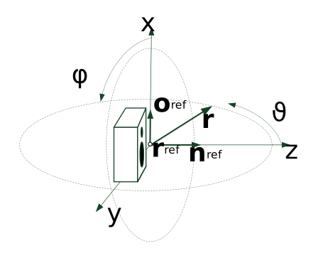
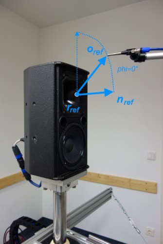
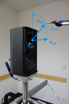
According to the standard the reference system is defined by the reference point \(r_{\text{ref}}\), the reference axis \(n_{\text{ref}}\) and the orientation vector \(o_{\text{ref}}\).
Reference Point#
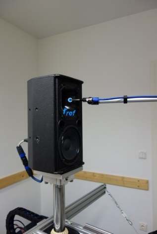
The Reference point is the origin of the acoustical coordinate system. Set it into the front plane and centered in front of the speaker. If it is not possible to move the microphone into the front plane, set it about 5 mm in centered in front of the speaker.
For systems with multiple speakers, it is recommended to set the reference point in front of the tweeter.
Move the microphone to the reference point. Select the reference point in the Setup Points Table and press “Save” to store the coordinates.
Reference Axis#
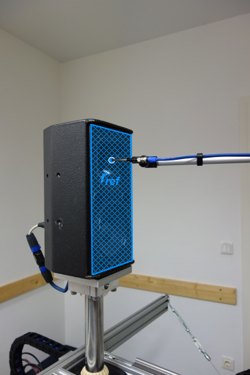
The reference axis define the main radiation axis of the device. To set it up, move microphone to a position of the main radiation axis, which is a few centimeters in front of the Reference Point. Select Reference Axis in the Setup Points Table and press save to store the coordinates.
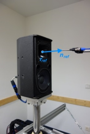
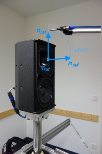
Orientation Vector#
The orientation vector defines the orientation of the device. It defines the circular angle of phi = 0°. In general, it points to the top. To set it up, drive the microphone in the orientation direction. Select Orientation Vector in the Setup Points Table and press save to store the coordinates.
The software detects the vector, which fitted the orientation direction best.
Click OK to confirm your setting and close the Hardware Setup window.
Configure the Measurement#
Click Edit Setup to open the Measurement Database.
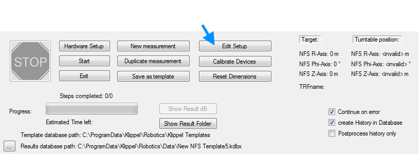
Select the Setup object.
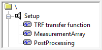
The object contains all operations for the measurement process. These are the generation of the grid (MeasurementArray) the measurement operation (TRF transfer function) and a PostProcessing.
TRF transfer function#
For this application, the TRF module is performing a measurement of the transfer function. In the following two basic configurations are described. For further information about the TRF module, please see TRF Manual.
Passive Speaker#
Connect Hardware
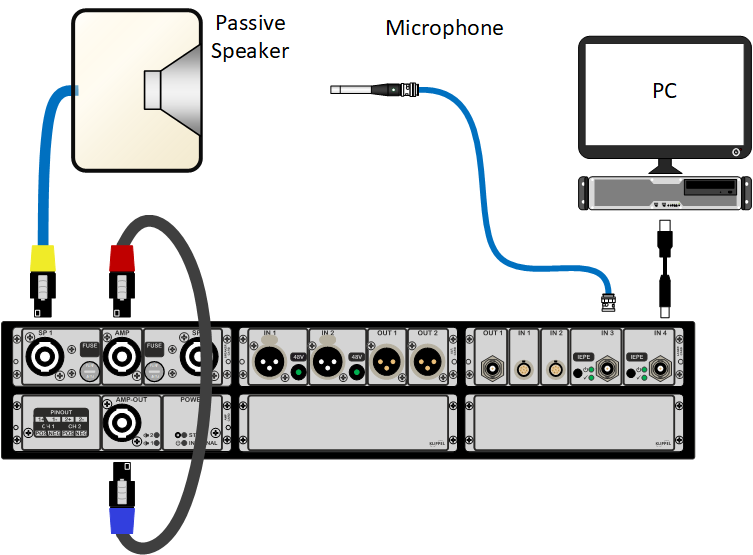
- Open Properties
- Open the properties window to configure the TRF operation.

- Configure Stimulus
- Select the Stimulus tab and define: Speaker 1 (via OUT1)Configure Parameters Frequency Range, Frequency resolution and Input Voltage for your device
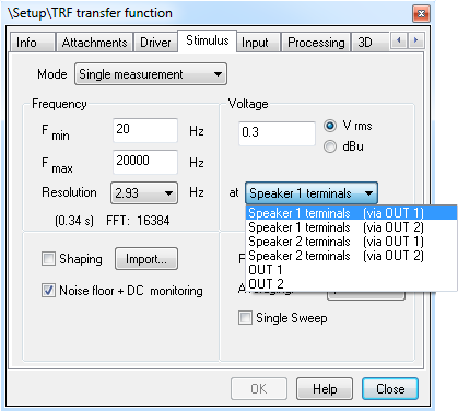
- Select Inputs
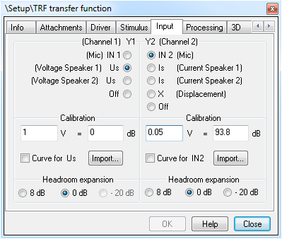
- 1) Select the Input tab and define:- Channel 1 - (Voltage Speaker 1) Us- Channel 2 - IN 2 (Mic)2) Insert the Calibration of the mic
- Define H(f)
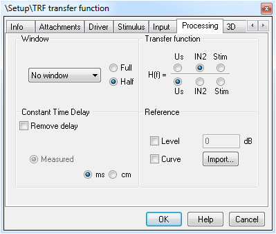
- Select the Processing Tab and define: H(f) = IN2 / Us
- Check Im/Export Tab
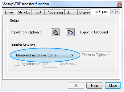
- Select the Im/Export tab.It is required for the NFS PostProcessing that the Measured Impulse Response is selected in Impulse Response” is selected in this tab. Make sure that the configuration is correct.
- Run Operation
- Run the TRF operation by clicking on the green arrow.
 The measurement should be performed in front of the loudspeaker. Move the microphone to the On-Axis position.
 - Check SNR
- Open the Result Windows Y1(f) Input Spectrum and Y2(f) Input Spectrum And check if the microphone signal has a SNR of at least 40 dB in the passband.
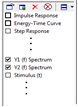 If the SNR is less increase the voltage of the Stimulus or apply averaging.
Active Speaker#
Connect Hardware
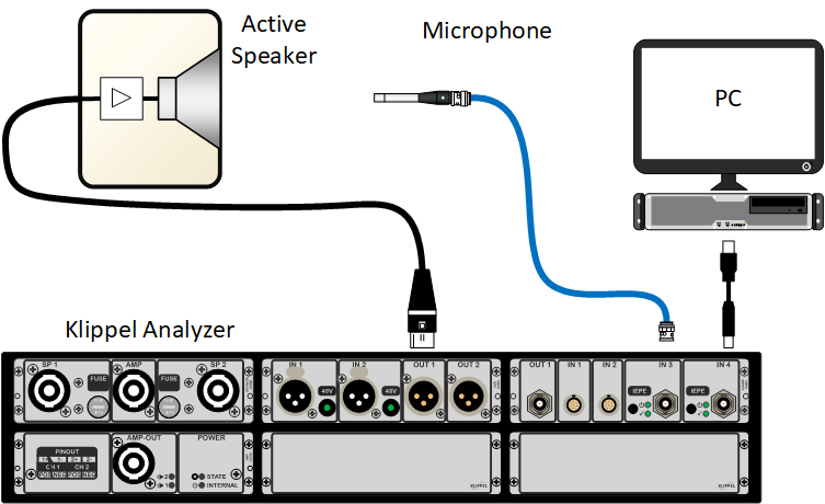
- Open Properties
- Open the properties window to configure the TRF operation.
- Configure Stimulus
- Select the Stimulus tab and define: OUT1Configure Parameters Frequency Range, Frequency resolution and Input Voltage for your device
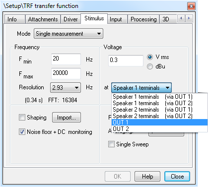
- Select Inputs
- 1) Select the Input tab and define:- Channel 1 - IN 1 (Mic)- Channel 2 - Off.2) Insert the Calibration of the mic
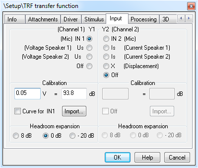
- Define H(f)
- Select the Processing Tab and define: H(f) = IN1 / Stim
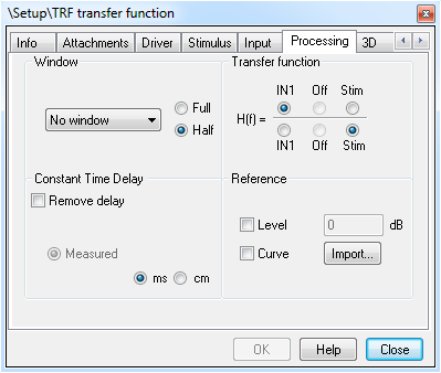
- Check Im/Export Tab
Select the Im/Export tab. It is required for the NFS PostProcessing that the Measured Impulse Response is selected in in this tab. Make sure that the configuration is correct.
- Run Operation
- Run the TRF operation by clicking on the green arrow.
The measurement should be performed in front of the loudspeaker. Move the microphone to the On-Axis position.
- Check SNR
- Open the Result Windows Y1(f) Input Spectrum and Y2(f) Input Spectrum And check if the microphone signal has a SNR of at least 40 dB in the passband.
If the SNR is less increase the voltage of the Stimulus or apply averaging.
Measurement Array#
The MeasurementArray generate the measurement grid. Open the properties window to configure the measurement grid.
All points that were defined in the Hardware Setup previously are imported automatically to the operation. The following parameters have to be defined in the Properties window. Please have a look at the Documentation window as well. There is a detailed description of the input parameters.
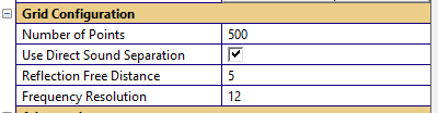
Parameters#
- Number of Points
Dependent from the device under test the following number of measurement points is recommended:
- Subwoofer
- Working Range: 10 Hz – 1 kHzNumber of Points: 300
- Full range Speaker
- Working Range: 20 Hz – 10 kHzNumber of Points: 500
- 2 way Speaker
- Working Range: 20 Hz – 20 kHzNumber of Points: 500 - 1000
- Professional Line array
- Working Range: 20 Hz – 20 kHzNumber of Points: 2500 - 3000
- Use Direct Sound Separation
The parameter “Use Direct Sound Separation” activates a second layer in the scanning grid. If you use the NFS in a non-anechoic ambience, it is required to check the parameter
- Use Direct Sound Separation ☐
- Ambience: anechoicScanning Grid: Single Layer
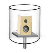
- Use Direct Sound Separation ☑
- Ambience: non-anechoicScanning Grid: Double Layer
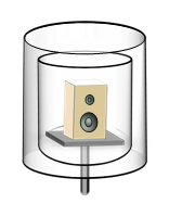
Note
The second cylindrical layer is 5 cm larger in r and z than the inner layer. Please check that the microphone can reach these positions without moving into the end switches.
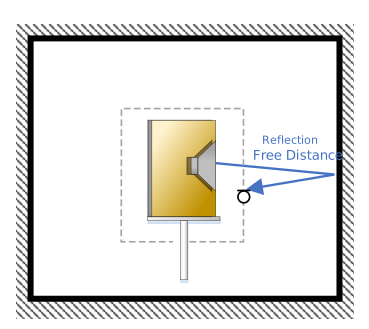
- Reflection Free Distance – covered distance of the first reflection
It is the distance from the sound source to first reflecting wall plus the distance back to the microphone position.
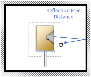
- Frequency Resolution
The parameter defines the frequency resolution of the results in points per octave. PointsPerOctave = 10 means, there are 10 frequency points in each octave.
Run operation#
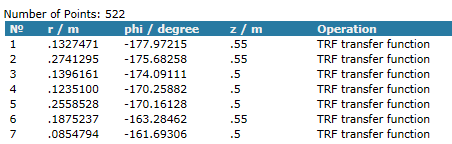
After finishing the definition of the parameter. Run  the Operation. The distribution of the measurement
points is visualized in the Result Windows.
the Operation. The distribution of the measurement
points is visualized in the Result Windows.
Note
In addition to the standard measurement, there are several possibilities to measure complex sound systems with the near field scanner. E.g. multiplexing multiple transducers of a line array. To see how this works please have a look at Application Note 70: Directivity of Speaker Array
Post Processing#
The PostProcessing organizes the data handling for each measurement. No settings have to be done in this operation.
Close the dB-Lab database to get back to the Robotics Software.
Start the Measurement#
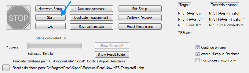
Press Start and a Dialog will appear.
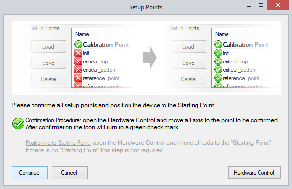
Confirm your settings with Continue to start the measurement.
The program starts with the calculation of measurement points. Dependent from the number of measurement points in can take several seconds. Subsequently the NFS will start to move.
Analyze measurement data#
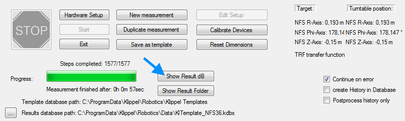
After finishing the measurement, all data is saved in the database. Select Show Results dB to open the Result Database.
Select Processing. As shown in the picture the Object Processing consists of three Operations. They are discussed in the following.
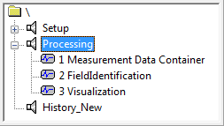
Measurement Data Container#
The Measurement Data Container stores all relevant data from the measurement, which are:
Coordinates and impulse response of each point
DUT position (reference point, main radiation axis, orientation, tweeter Point)
Measurement Room (Reflection Free Distance, Field Separation required)
Target Frequency Resolution
Measurement information (Frequency Range, Microphone Sensitivity, etc.)
The Measurement Information is imported automatically and can be edited in the Property Page
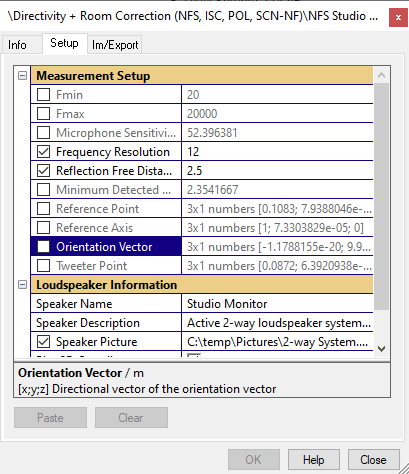
In addition to the imported parameters, information about the device (Name, Description, Picture) can be stored as well. For further information, please see the Documentation Window.
Run
the script and the open the Summary window. This is showing basic information about
the Measurement Data Container.
Field Identification#
Select the operation 2 Field Identification and open the Property Page. The Following parameters are important to run an identification.
- Order of Expansion
Select “Order of Expansion” and open the edit window. Running the Field Identification for the first time, it is recommended to start with the default configuration as shown in the picture.
- Direct Sound Separation
If the measurement was performed in a non-anechoic room, activate this parameter.
Run Field Identification#
Click Run  to start the operation. The calculation may take several minutes.
Results of Field Identification#
After finishing the calculation have a look at the result Windows. (For a detailed description please see Holographic Field Identification)
Optimize settings and verify results#
Check Fitting Error#
The fitting error characterize the accuracy of the sound field identification. It describes the difference of the identified sound field and the measured transfer function at the measurement surface. The curve show the Fitting error in dB. It is calculated by:
In general the fitting error is supposed to be below -20 dB, which is an error on 1 %. But it is always important to check the other measures because the fitting error is a relative error and depends on the radiated sound pressure level. That means, is the radiated sound pressure very low and the microphone signal is close to the noise floor, the fitting error rises.
The following example shows the fitting error over frequency:
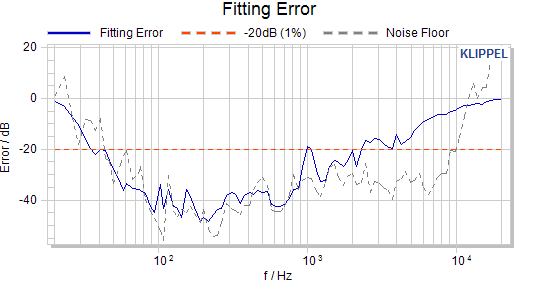
As seen in the picture, the noise floor increases at the lower and the higher end of the frequency band. The device is out of the passband. In this region the fitting error increases as well, because it’s influenced by noise. From 50 Hz to 2 kHz the sound field can be identified accurately, the fitting error is always below -20 dB. Above 1 kHz the fitting error rises but the SNR is still OK. In this frequency band a higher order of spherical harmonics is required to identify the sound field.
Check H(f) Magnitude window#
Using the Field Separation, the direct sound is separated by two different methods.
For high frequencies, the common gating technique is used to cut off room reflections. The Reflection Free Frequency \(f_{\text{RF}}\) defines the lower limit of the frequency band where gating can be applied.
For low frequencies, gating cannot be applied. Therefore, the direct sound have to be separated by holographic methods. The frequency band of the holographic field separation has an upper limit \(f_{\text{FSmax}}\).
Reflection Free Frequency \(f_{\text{RF}}\) is smaller than the Field Separation Limit \(f_{\text{FSmax}}\)
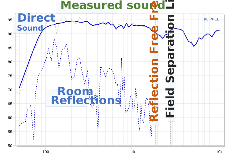
Sound field can be identified over the whole frequency band.
Reflection Free Frequency \(f_{\text{RF}}\) is greater than the Field Separation Limit \(f_{\text{FSmax}}\)
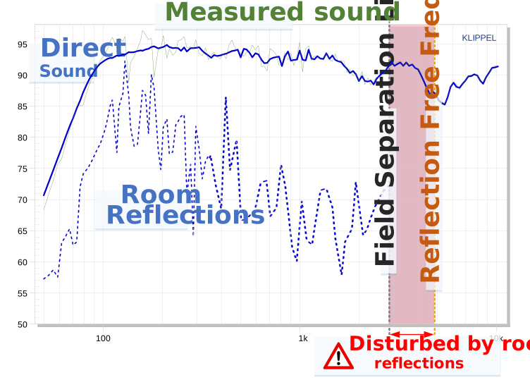
The result might have errors in the frequency band between Reflection Free Frequency and Field Separation Limit
Visualization#
Select the Visualization Operation and open the Property page and ensure the correct Field Identification is linked for the analysis.
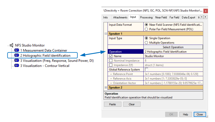
Close the Properties Window and “Run”  the Visualization Module. For detailed description of
the handling of visualization software, please see Part 1 - Viewing NFS Results
the Visualization Module. For detailed description of
the handling of visualization software, please see Part 1 - Viewing NFS Results
Part 3: Asynchronous and Open Loop Testing#
What is the goal of this tutorial?#
For audio devices that don’t have an analog input the measurement stimulus needs be transmitted via a wireless connection or is played by the device under test itself.
This Tutorial discussed the particularities of a measurement of a Bluetooth® loudspeaker using the Near Field Scanner measurement system. Other wireless devices (e.g. Wifi) can be measured similar.
It’s required to do Tutorial Part 2 before which covers a detailed description of the complete measurement procedure.
Additional Hardware Required#
Bluetooth® Transmitter#
3rd party Bluetooth® transmitter with an analog input (e.g. 3.5mm jack) or digital input (e.g. SPDIF). It can be either a professional transmitter or a common consumer product
2nd Microphone#
2 microphones are required to perform an asynchronous measurement.
Microphone 1: Test microphone of the NFS
Microphone 2: Used for synchronization
Measurement Setup#
The NFS supports two setup for asynchronous measurement. The measurement with an external transmitter and open loop measurement. Both setups require a 2nd microphone that is used to synchronize of the impulse responses of the main measurement (Microphone 1).
Note
Wireless connections often has variable delays that need be considered to ensure an accurate phase measurement
For this reason the microphone 2 must be at a fixed position. Please mount microphone 2 on the platform in the center of the Near Field Scanner in front of the DUT.
Mounting recommendation of the synchronization microphone#
Full space measurement (4π)
The synchronization microphone must be very close to the device under test to get high SNR and robust measurement conditions. In addition, it shouldn’t disturb the measure by its physical presence. That’s why Klippel is offering a special capsule microphone (GRAS 47AX), which can be mounted easily close to the DUT and has a minimum influence on the measurement.
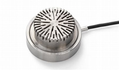
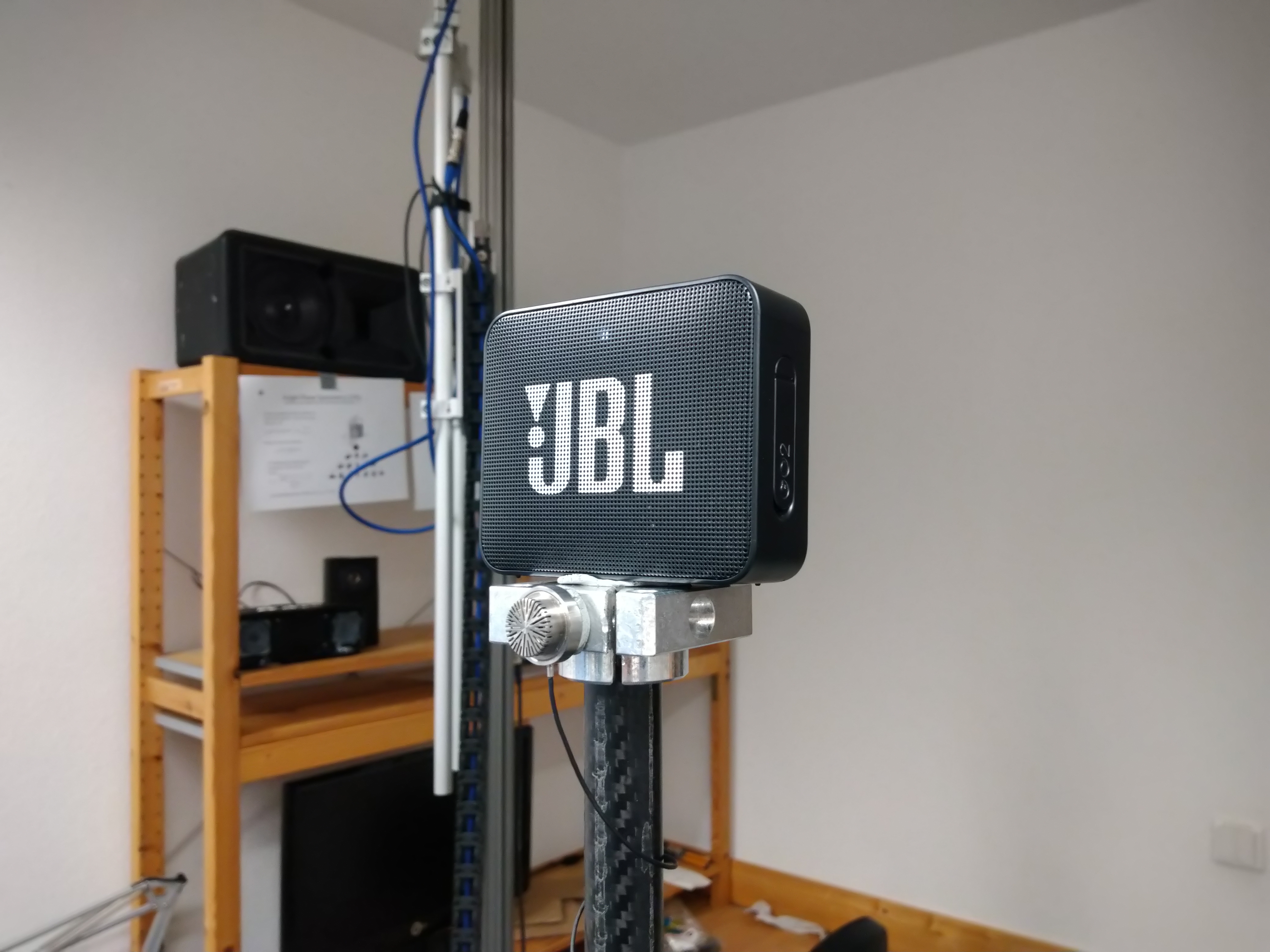
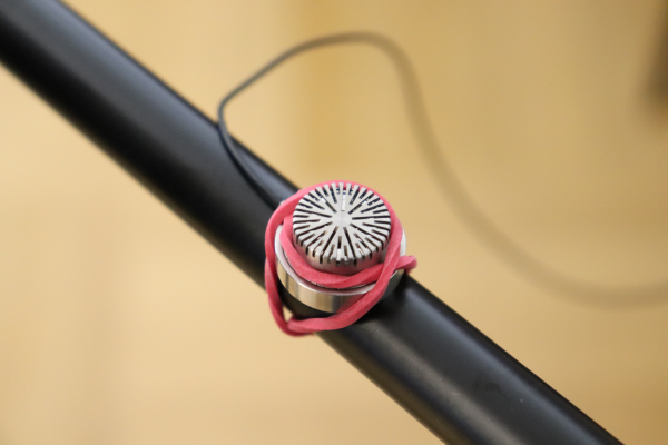
Note
Other measurement microphones can be also used as a synchronization mic, but the mechanical mounting might be a bit more complicated.
Half space measurement (2π)
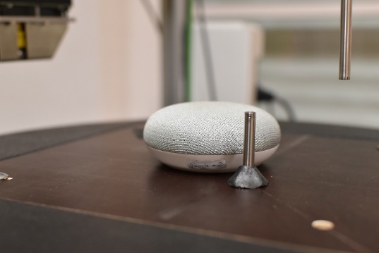
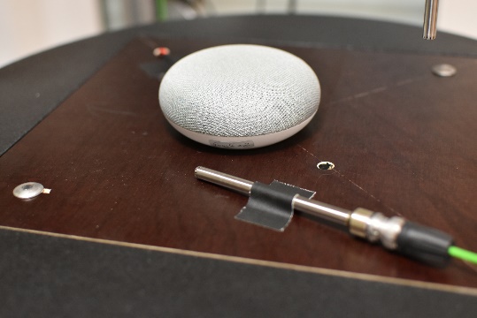
For the baffle scan the mounting of the synchronization microphone is usually simpler. The microphone can be mounted for example by drilling additional hole in baffle and mount it from the back side (left) or it can be fixed directly on the baffle (right). The GRAS 47AX could be also used for that application.
Setup 1: Measurement with Bluetooth® transmitter#
Analog output of the Klippel Analyzer is connected to a Bluetooth® transmitter, which sends the signal to the device under test.
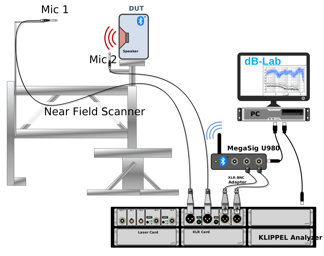
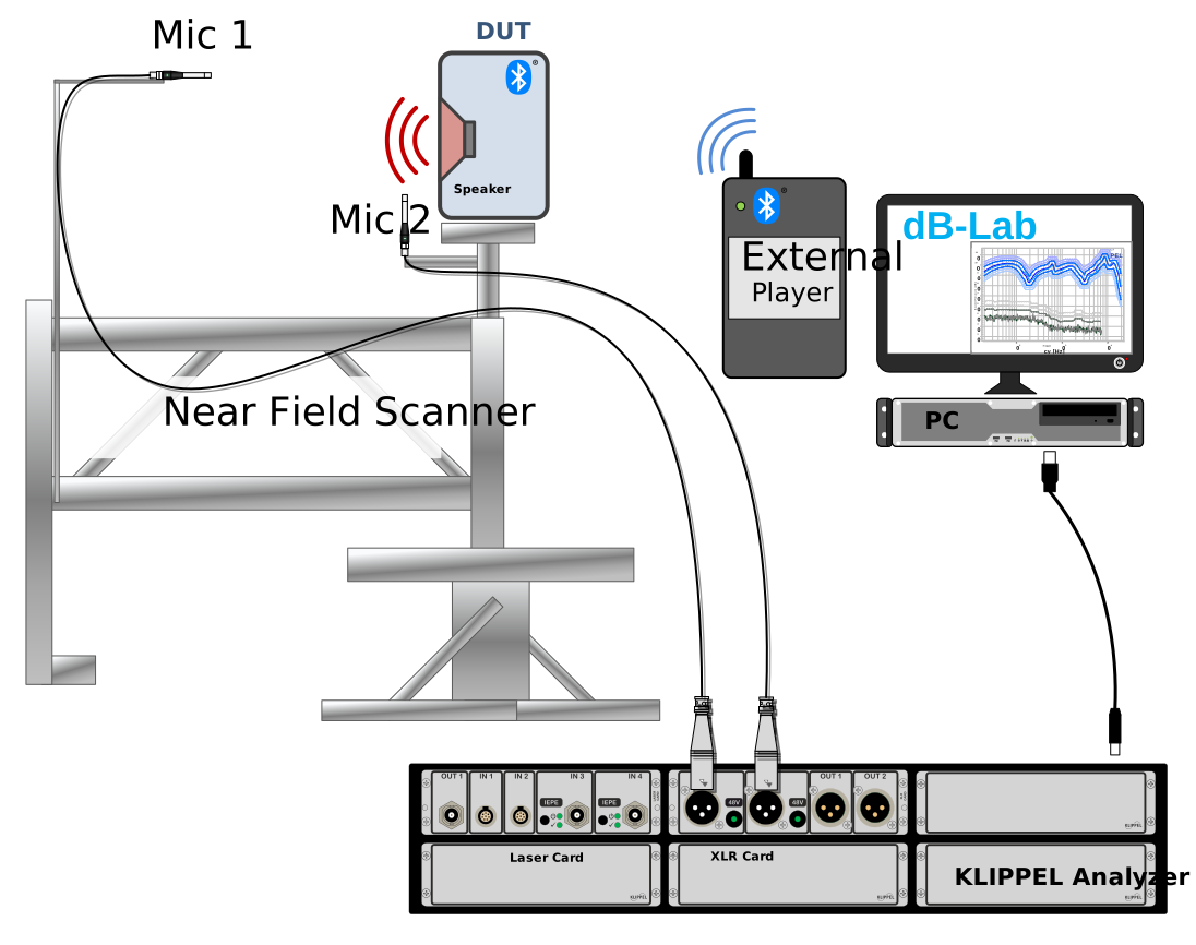
Setup 2: Open Loop Testing#
Stimulus is played as a looped wav-file with an external player or directly on the device under test.
Measurement Template#
Open Robotics Software and click: New Measurement
For the different holographic measurement application (NFS, NFS Baffle, kl-scn Near Field Add-on) there are Bluetooth® templates. Use the corresponding template for your measurement application.
Hardware Setup#
The Hardware Setup is identical to a standard NFS measurement. Please see Initialize Near Field Scanner Hardware
Configure the Measurement#
Click Edit Setup to open the Measurement Database
Measurement Array#
Select the Measurement Array operation and open the Property Page. Select the tab Asynchronous Measurement and check the following parameters:
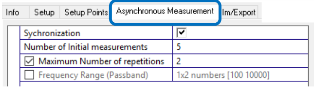
- Synchronization
This parameter must be activated for an asynchronous measurement.
- Number of Initial Measurements
At the beginning of the Scan a few measurements are repeated to determine the response of the synchronization microphone (Mic2). This data is used to check validity of the measurements during the scan.
- Maximum number of Repetition
Probably a few measurement will be disturbed during the scanning. This can be caused by transmission problem of the wireless connection. The NFS repeats automatically these disturbed points at the end of the scan. Using this parameter it can be defined how often a point will be measured again.
- Frequency Range (Passband)
The passband of the device can defined to limit the checks to that frequency range. If this is not specified this range will be detected automatically.
Note
The other setting of Measurement Array operation (e.g. Grid Configuration) are similar to a standard NFS measurement procedure. Please for more details see the corresponding applications
TRF Transfer function#
Stimulus Settings#
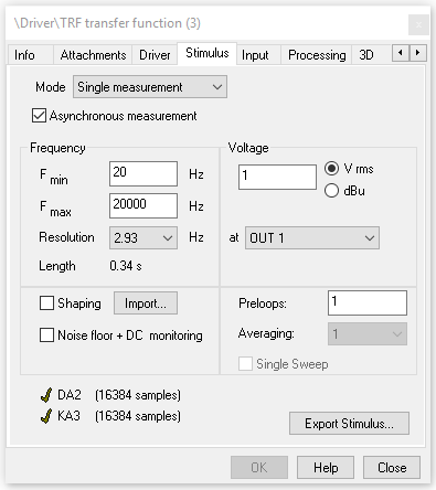
Select the Stimulus tab and check the following parameters:
Asynchronous measurement must be activated
Select OUT1
Frequency range and input voltage (dependent on DUT):
Frequency Range (fmin, fmax)
Frequency Resolution
Input Voltage
Stimulus Export (only for open loop testing)#
Measuring in an open loop setup the test stimulus needs to be exported to the device under test. To do this the TRF module has an export function.
Click Export Stimulus to save the test signal as a wav-file. For a NFS measurement choose the maximum length of 25 min.
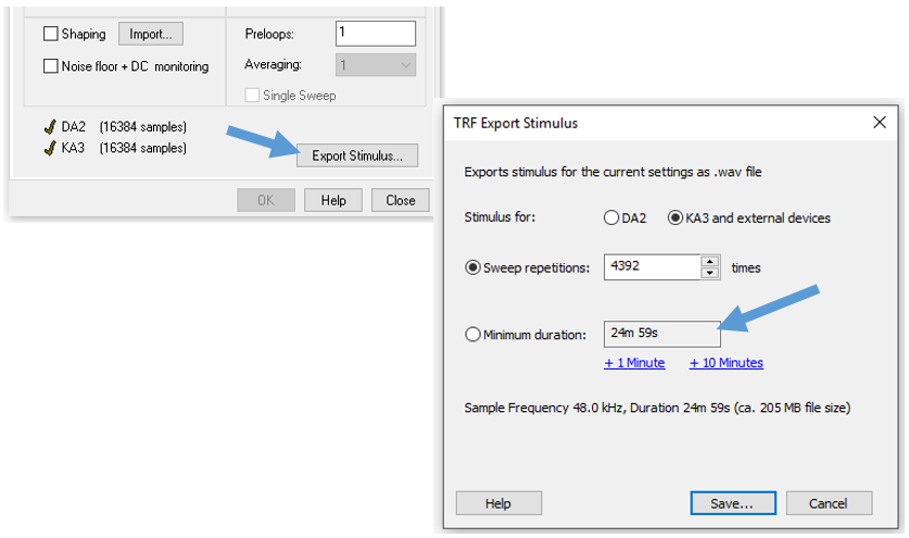
After exporting stimulus do not change the settings of the sweep.
Inputs#
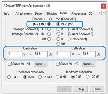
Select the Input tab and define:
Channel 1 – IN 1 (Mic): NFS Measurement Microphone (moving)
Channel 2 - IN 2 (Mic): Synchronization Microphone (fixed position)
Also specify the sensitivity of both microphones.
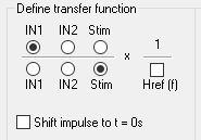
Transfer function#
Select the Processing Tab and define: H(f)= IN1 / Stimulus
Make sure that the checkbox Shift Impulse to t=0s is not activated.
Perform Test Measurement#
Setup 1: Pair Speaker and Transmitter#
Pair the device with the transmitter. It is recommended to check the wireless connection before starting the measurement. This can be done with music.
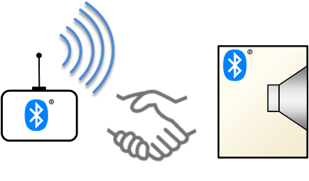
Listen carefully and check with the music that the connection is stable and there are no audible dropouts. If everything is okay, connect the Analyzer.
Setup 2: Play Stimulus on device#
Start the playback of the Stimulus on the device.
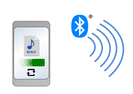
Make sure the player has an auto repeat function, because the NFS measurement will take longer than the length of the wav file.
Run the TRF operation and check the results of the measurement.#
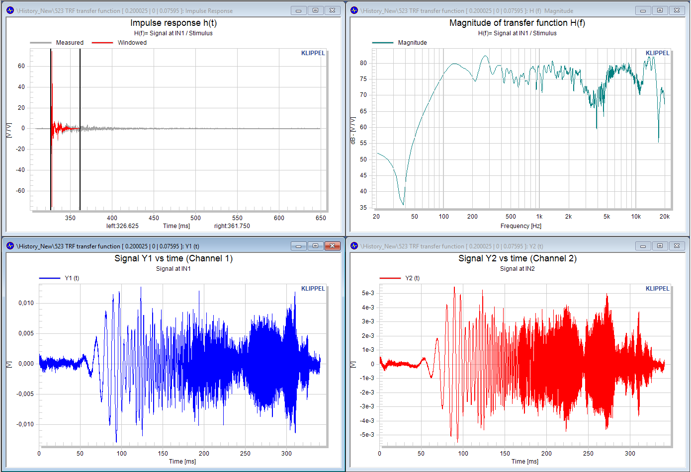
Make sure both microphones has a good signal to noise ratio. This can be done by checking the transfer function and impulse response of both channels.
Start Measurement#
Close the database to get back to the Robotics.
It’s recommended to activate Create History in Database to store all individual TRF measurements during the scan. In case of unpredictable problem during the measurement (e.g. dropout in the wireless connection) this data can be very valuable to find the root cause.
Press Start to run the measurement.
Note
For open loop measurements, don’t forget to start the playback of the stimulus.
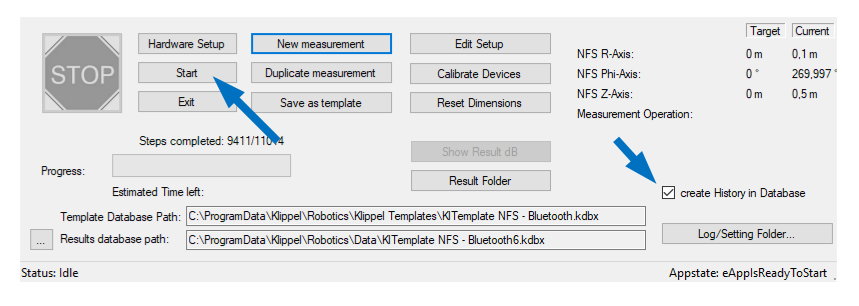
Analyze Measurement Data#
After finishing the measurement, all data is saved in the database. Select Show Results dB to open the Result Database.
The analysis procedure is similar to a standard NFS measurement and is described in Tutorial Part 2. See Analyze measurement data.
Part 4: Half Space Measurement#
What is the goal of this tutorial?#
To determine the acoustical output of a transducer without the influence the speaker cabinet, the speaker is measured in a baffle. Also for many consumer loudspeaker systems half space is important because these smart devices are often operated on a table. This Tutorial shows how to perform such a half space measurements with the Near Field Scanner, acquiring the 3D sound pressure output of a transducer or smart devices.
Note
It’s required to do Tutorial Part 2 before which covers a detailed description of the complete measurement procedure and the calibration of the measurement hardware.
Additional Hardware Required#
The half space measurement requires a hardware add-on. Basically a half space measurement can be performed in 2 different configurations.
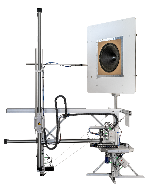
- Vertical Baffle
- For a vertical mounting of transducers Klippel provides the NFS Baffle hardware add-on, which combines a flexible light weight structure with the high requirements for acoustical measurement.
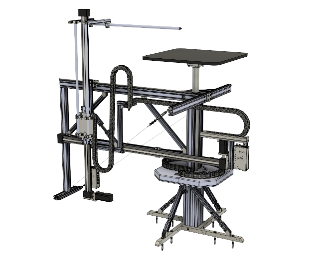
- Horizontal Baffle
- As an alternative a custom baffle can be also mounted horizontally on the NFS. In addition to scanning transducers such a setup can be used to measure small loudspeaker systems (e.g. Smart speaker) in a ground floor setup.
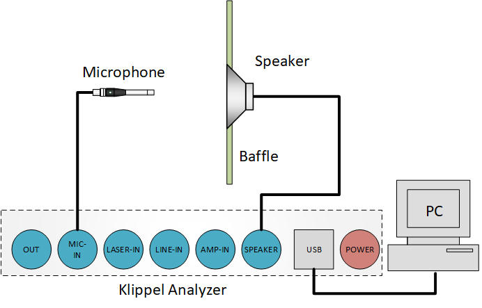
Measurement Setup#
Note
Also wireless testing in half space is supported. For details see Part 3: Asynchronous and Open Loop Testing
Measurement Template#
Open Robotics Software and click: New Measurement
Dependent if you are using a vertical or horizontal baffle select the corresponding template.
Hardware Setup#
Similar to a standard NFS measurement the Axes of the Near Field Scanner need to be initialized and the microphone position must be calibrated. For more details about this procedure please see Part 2: Perform a Measurement.
Vertical Baffle#
This section is describing the setup using a vertical baffle. In case you are using the horizontal setup go to Additional Hardware Required.
Setup Points#
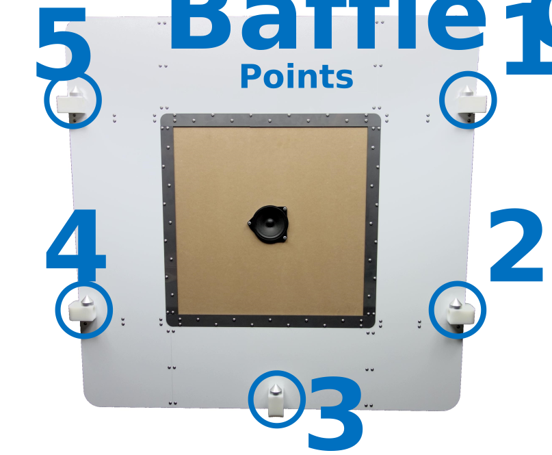
To perform a half space scan the exact position of the baffle need to be specified. This is done by moving the microphone to specific position in front of the baffle. Using the calibration cone holder and the calibration cone, a defined distance to the baffle can be measured accurately.
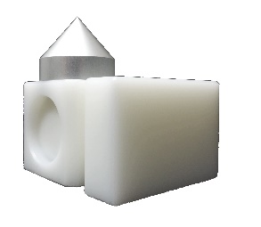
Please put the calibration cone to the following positions.
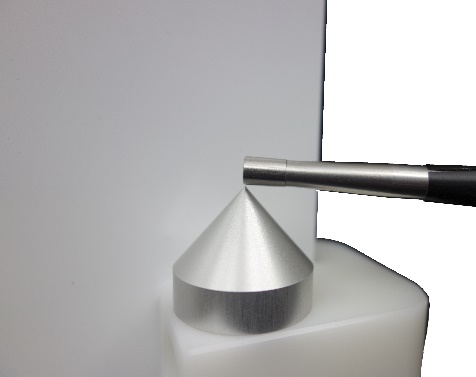
Use the remote control to move the microphone to the tip of the cone for each point.
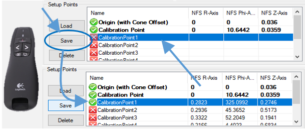
Save the coordinates by using the Setup Points dialog.
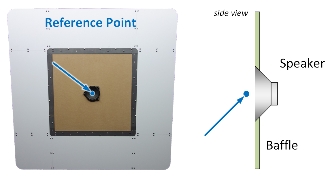
To the set Reference Point move the microphone in front of the transducer.
Configure the Measurement#
Click Edit Setup to open the Measurement Database
Measurement Array#
Select the Measurement Array operation and open the Property Page.
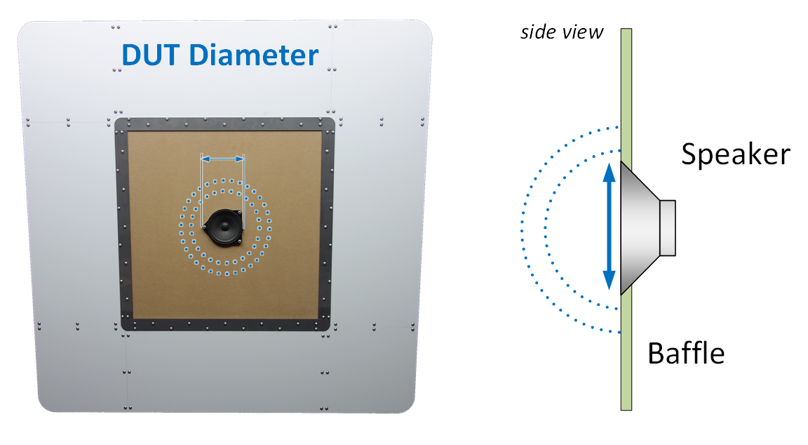
The NFS Baffle measurement is performing a scan on a hemispherical surface in front of the driver. Dependent on the DUT the diameter needs to be specified. The scan will be performed on 2 layers to separate the room reflections as well as the acoustical short and the diffraction effects from the baffle in the further holographic processing.
Distance to Calibration Plane#
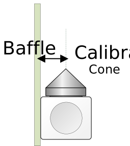
Also check that the Distance to the Calibration Plane is correct. Using the Klippel Calibration cone holder this distance is exactly 20mm.
It’s is important to specify this number accurate to identify the baffle position.
Safety Distance#
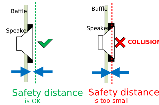
To avoid a collision with the baffle also a Safety Distance need to add. To set this parameter please measure the highest part of the loudspeaker that protrudes out of the baffle.
Run the MeasurementArray operation to calculate the coordinates and check the calibration of the baffle position.
Baffle Calibration Check#
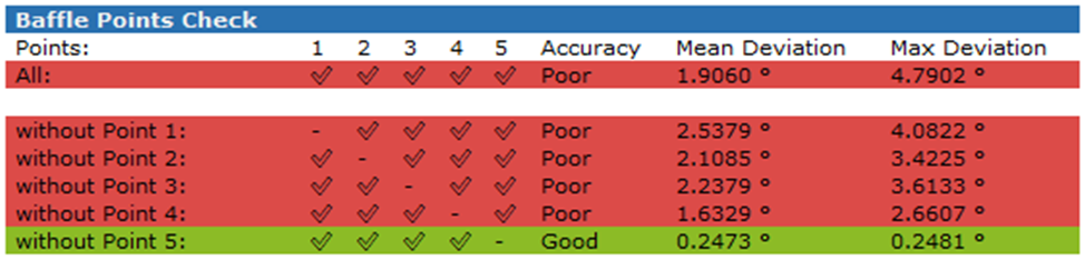
The window Baffle Calibration Check shows the result of the automatic verification of the baffle points.
- Good Accuracy:
If all points are set correctly the table shows a good accuracy of the baffle calibration points, which means that all points are in a plane.

- Medium Accuracy:
If the Table shows a result with medium Accuracy the Baffle Scan can also be performed. But the points could be defined more accurate

Note
When only a medium accuracy was reached please see the additional information and remeasure only the point which has the highest error.

- Poor Accuracy
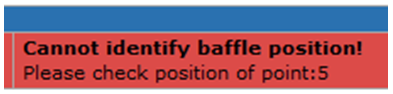
This verdict shows that the Baffle Calibration are not in a plane. To avoid collision the scan cannot be performed with this setting.
Note
Very often only a single point has a wrong setting and need to be remeasured. Please see the error messages for more information.
Horizontal Baffle#
Setup Points#
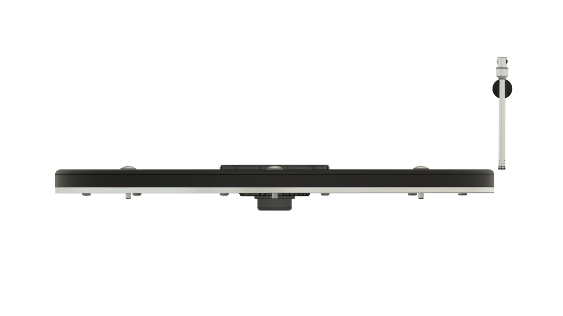
Using the horizontal setup the height of the baffle need to be specified. To do this use the remote control to move the microphone to the exact height of the baffle. To avoid collision during that process, it is recommended to move the microphone outwards to the side of the plate.
Configure the Measurement#
Click Edit Setup to open the Measurement Database
Specify DUT#
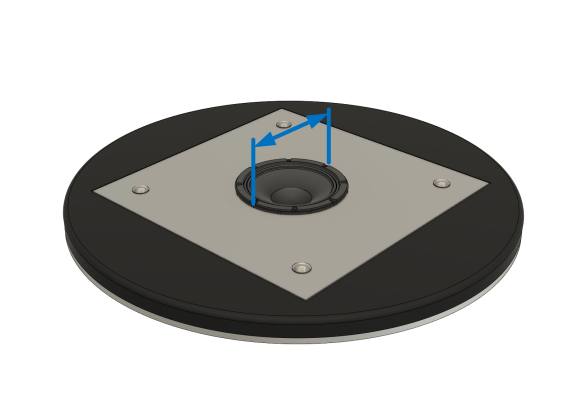
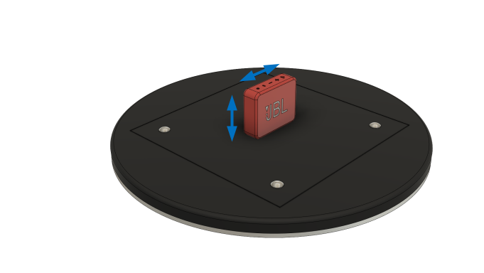
Select the Measurement Array operation and open the Property Page. In the Category Grid Configuration, you can select the type of Device. This can be either a transducer mounted flat into the baffle or a compact device standing on the plate (e.g. smart speaker)
To specify the size of the scanning grid, set either the diameter of the transducer or the diameter and the height of the compact device.
- Transducer
- Compact device
Safety Distance to Baffle#
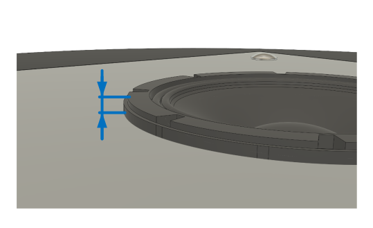
The Safety Distance to the baffle defines a height beneath which points are not measured in order to avoid collision between the microphone and the baffle or slightly protruding DUTs. Measure and enter the height of Transducer Type DUTs, cables for active DUTs or any other obstructions on top of the baffle.
Calculate grid#
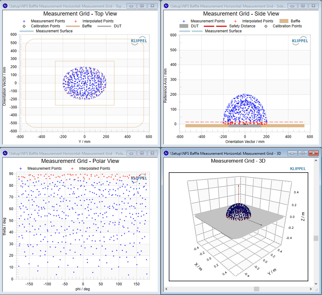
Press run to generate the measurement grid. After running the operation the measurement points are visualized in the result windows.
TRF Transfer function#
The transfer function setting are identical to a standard NFS measurement with a passive speaker. For further information please see Tutorial Part 2. For wireless testing see Tutorial Part 3 for setup details.
Start Measurement#
Close the database to get back to the Robotics and press Start to run the measurement.
Analyze Measurement Data#
After finishing the measurement, all data is saved in the database. Select “Show Results dB” to open the Result Database.
Field Identification#
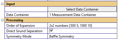
The analysis of the measurement data is almost identical to a standard NFS measurement. The only thing which need to set is the Symmetry Mode: Baffle Symmetry and the Direct Sound Separation to remove the baffle effects as well as the room reflections.
For more information see Tutorial Part 2 (see Analyze measurement data).
NFS – Reference#
NFS Measurement#
Measurement Process#
The measurement process is structured into data acquisition and data preprocessing. Transfer function measurements are done on multiple positions along a surface very close to the sound source.
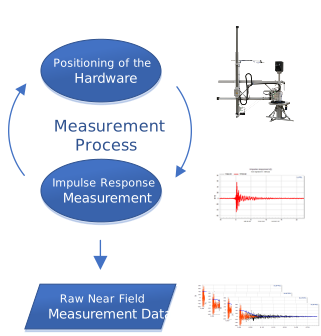
According to the required Setup, a grid of measurement points is calculated. The System automatically positions the hardware and runs a measurement of the Impulse response at every single point.
Coordinate System#
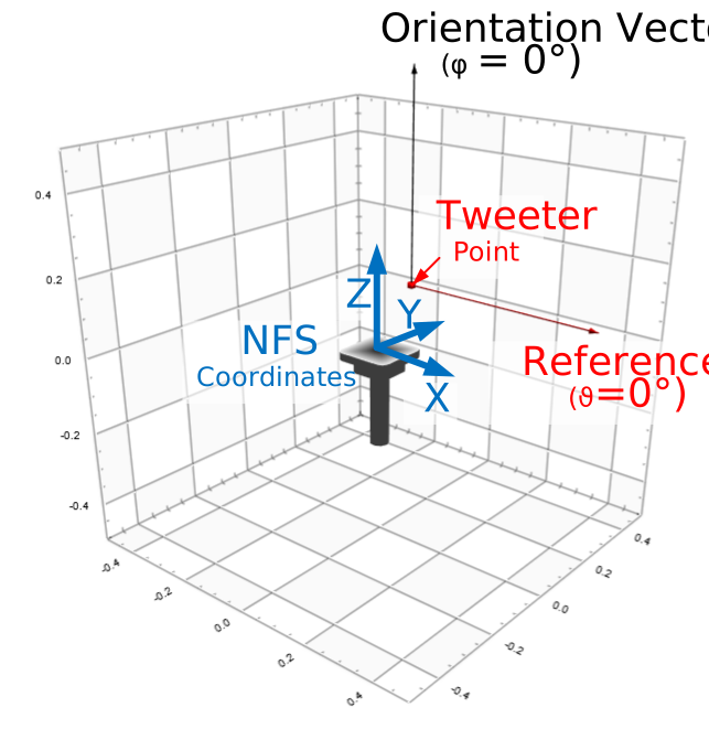
The reference system defines the acoustical coordinate system, based on the IEC standard 60268-21. According to the standard, the reference system is defined by the reference point \(r_{\text{ref}}\), the reference axis \(n_{\text{ref}}\) and the orientation vector \(o_{\text{ref}}\).
Parameter#
Measurement Setup#
- Operation List
List of all operations that will be performed during the scanning process. How it works?
Select Operation or Create a New Operation
Configure the parameter of the UI (e.g. Measurement Operation & MUX Settings
Save Operation in List
Operation is added to Operation List
When selecting an operation of the list, the interface of the properties window is updated and will show the operation settings.
- Measurement Module
The parameter defines the measurement operation, which will be performed. [e.g. ‘TRF Transfer Function’]
- Use Multiplexer
Activate multiplexer interface
- Select Multiplexer
Select a device from the list of all available multiplexers
- MUX – Activate
Boolean to active the selected multiplexer:
☑ checked: MUX is activated
☐ not checked: MUX is deactivated
- MUX – Mode
Parameter to select the switching mode of the multiplexer. The following option are available:
o 1x8: one of the inputs is routed to A and B
o 2x4: parallel switching of A (Ch. 1-4) and B (Ch. 5-8)
o 4+4: separate routing of Ch. 1-4 to A and Ch. 5-8 to B
o Custom: Custom configuration
- MUX – Channel1
Routing of output A and B for MUX-Mode ”1x8” or
Routing of output A for MUX-Mode ”2x4” and “4+4”
- MUX – Channel2
Routing of output B for the MUX-Mode “4+4”
- MUX – IEPE Ch. 1-4 (BNC-MUX only)
Activates IEPE for Channel 1-4 for a microphone MUX
(MUX81-42-BNC - Art.No.:2800-101)
- MUX – IEPE Ch. 5-8 (BNC-MUX only)
Activates IEPE for Channel 5-8 for a microphone MUX
(MUX81-42-BNC - Art.No.:2800-101)
- MUX – Custom Command
List of commands for the MUX, for the advanced usage. Using this parameter any possible multiplexer configuration can be switched. See the following example:
'set1x8 5'   // in 5 with 1x8 mode to out A and B
'seticp 2 1' //activate IEPE supply for Channel 5-8
- MUX – Switch Configuration
By clicking the button, the current MUX configuration will be send to the multiplexer devices and the hardware will switch.
- File Execution
Path of a file (e.g. *.bat) that is executed before the measurement.
- Transducer Position/Name
For measuring multiple transducer separately during one scan, a transducer name can be added to save the measurement results in separate data containers.
- Tweeter Point
Specify the position of the transducer based on the saved MUX Tweeter points
- Number of Measurement Points
Number of measurement point for the defined transducer If this parameter is defined, the total number of measurement points will be ignored
- Save Operation in List
Controller to save current configuration in the Operation List
- Delete Operation
Use this controller to delete the selected measurement operation form the Operation List.
- Delete All Operation
The controller resets the Operation List
Grid Configuration#
- Number of Points
Number of Measurement Points
- Use Direct Sound Separation
If activated, a double layer grid is generated, required for the measurement under non-anechoic conditions.
The 2nd layer is 5cm larger than the inner layer, which is defined by the setup points.
- Reflection Free Distance
- \(d_{\text{rf}}\) in \({m}\)The parameter defines the covered distance of the first reflecting sound wave.
- Frequency Resolution
- \(\Delta f\) in \(\text{points/octave}\)The parameter defines the target frequency resolution in points per octave. For Example:
24 points per octave 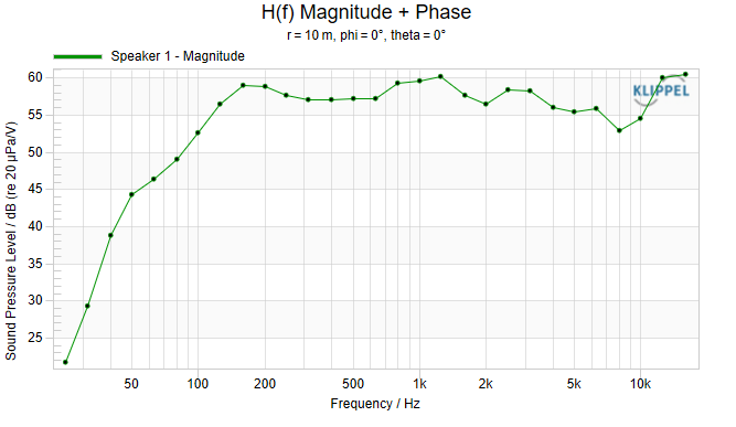
3 points per octave
Setup Points#
- Critical Point Bottom
The parameter defines the lower limit surface of the cylinder and the minimum radius on the lower surface To avoid collision between the microphone and the stand, make sure the point is the speaker platform and that the microphone will not hit the pole. Also make sure that all obstacles (e.g. cables) are above the z-position or inside the r-position. See the following examples.
- Tweeter Point
The tweeter point defines the origin of the spherical wave expansion. It is supposed be in front of the tweeter (close to the acoustical center for high frequencies).
- Starting Point
The Parameter defines the upper limit of the surface and the radius of the cylinder.
To avoid collision make sure that all obstacle (e.g. enclosure, cables ) are below the z position and inside the radius of the Starting Point. See the following examples.
- Critical Point Top (optional)
The parameter defines the minimum radius on the upper surface.
It is required for an overhanging Setup, when the device in mounted in the ceiling or on a crane. For such a setup there is an area on the upper surface which can’t be reached by the microphone. See the following examples:
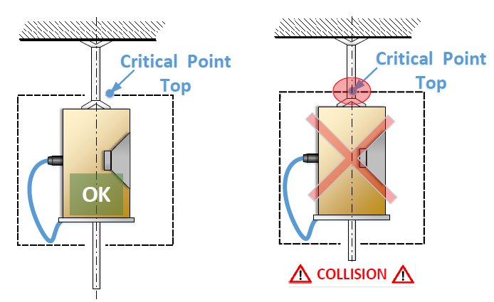
Reference Points#
- Reference Point (optional)
The Reference point is the origin of the acoustical coordinate system. Set it into the front plane and centered in front of the speaker. If it is not possible to move the microphone into the front plane, set it about 5 mm in centered in front of the speaker. For systems with multiple speakers, it is recommended to set the reference point in front of the tweeter.
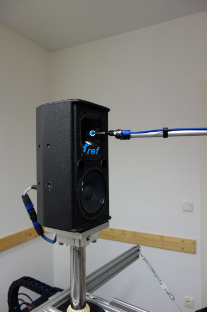
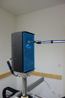
- Reference Axis (optional)
The reference axis defines the main radiation axis of the device. To set it up, move microphone to a position of the main radiation axis, which is in front of the Reference Point.
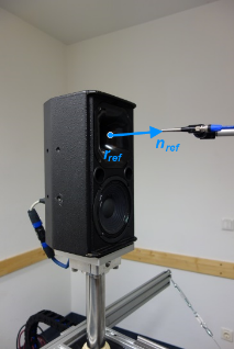
- Orientation Vector (optional)
The orientation vector defines the orientation of the device. It defines the circular angle of phi=0°. In general, it points to the top. The software detects the vector, which fitted the orientation direction best.
Advanced#
- Driving Job
Parameter to modify the movement order of the scan. The Measurement points can be optimized to minimal movement, sorted so that each transducer is measured in one pass, or sorted so that the rough scan is performed first.
- Parking Position
Selects where the scanner moves after finishing the measurement.
Options:
Automatic: Automatic parking at phi = 0°
Custom: Explicit coordinates defined by “Parking Position (R)”, “Parking Position (PHI)” and “Parking Position (Z)”. The coordinates must be outside the measurement surface to avoid collisions.
On-Axis: NFS moves to the On-Axis position after the scan. The distance to reference points is defined by “Parking On-Axis Distance”.
- Parking On-Axis Distance
Distance in meters used when “Parking Position” is set to “On-Axis”. This value defines the distance to the reference point along the reference axis. Ensure the resulting parking coordinates are outside the measurement surface.
- Parking Position (R)
After the Scan is finished the NFS will move to that position. To prevent any collisions with the Device Under Test (DUT), the R-Position must be beyond the scanning surface, ensuring a radius larger than the measurement cylinder.
- Parking Position (PHI)
After the Scan is finished the NFS will move to that position.
- Parking Position (Z)
After the Scan is finished the NFS will move to that position.
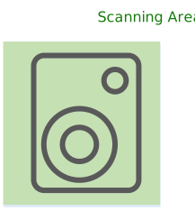
Symmetry#
Option to assume symmetry features for the measured device. The following symmetries can be applied to the Scanning grid:
- No Symmetry
- Half Sphere
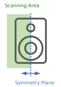
Horizontal - Right 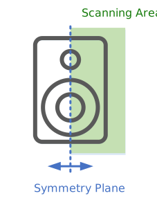
Horizontal - Left 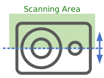
Vertical - Upper 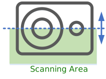
Vertical - Lower
Quarter Sphere
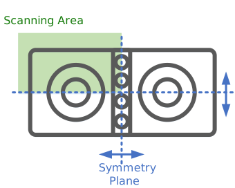
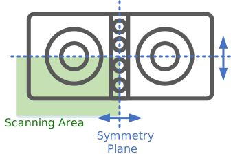
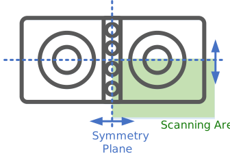
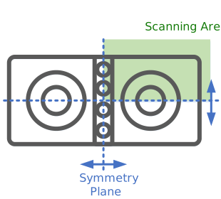
Note
Using direct sound separation, the measurement grid will always include a rough scan over the complete cylinder. This is necessary to identify the room reflections that are usually not matching the symmetry of the DUT.
Mux Tweeter Points#
Positions of the transducer for measurement with multiplexer. It’s recommended to define
Asynchronous Measurement#
For measuring devices with variable delay e.g., loudspeaker with Bluetooth® wireless technology, the scanning needs a second microphone to synchronize the measurement.
For more details see Tutorial Part 3: Asynchronous and Open Loop Testing
- Synchronization
If checked the synchronization is activated. For this option a second microphone is needed.
- Number of Initial Measurements
Number of Initial measurements to calibrate the response of microphone 2 for ambient noise check and synchronization
- Maximum Number of Repetitions
Defines how often a disturbed measurement point will be repeated. If deactivated the measurement will continue the measurement until all points were measured successfully.
- Frequency Range (Passband)
Frequency Range of the device under test [Fmin Fmax].
In this Frequency range the reliability of the measurement will be checked. If not defined, the Frequency Range is set automatically
Results#
Table of Coordinates#
The result window shows all measurement positions and information about the selected measurement operations. This way, you have the possibility to check if the grid meets your expectations. The results table looks similar to the following picture:
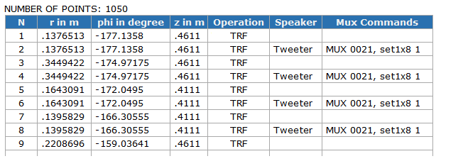
The columns of the table have following meaning:
- column 1
- N number of the measurement point
- columns 2-4
- contain the measurement coordinates (r,phi,z)
- column 5
- Measurement Operation that is performed
- column 6
- Name of transducer
- column 7
- Multiplexer Commands
Measurement Points#
The other result windows visualize the distribution of the measurement points on the three surfaces (Top, Lateral and Bottom) and as a side view.
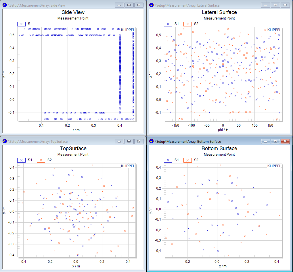
Measurement Data Container#
After the measurement is done, all the measured impulse responses and the coordinates of the measurement points are stored in the Measurement Data Container.
Most parameters are defined before the measurement and will be imported from the Data Container and transferred automatically into the Field Identification module. However, all settings can be edited in the Data Container Operation.
Parameter#
- Minimum Frequency
- \(f_{min}\) in \(\text{Hz}\)Minimum excitation frequency of the transfer functions measurement TRF (Imported from TRF)
- Maximum Frequency
- \(f_{max}\) in \(\text{Hz}\)Maximum excitation frequency of the transfer functions measurement TRF (Imported from TRF)
- Microphone Sensitivity
- \(\text{mV/Pa}\)Definition of the calibration factor of the microphone in mV /Pa (Imported from TRF)
- Microphone Frequency Response
- Defines the variation of microphone sensitivity over frequency.
Format:
Frequency [Hz] |   Level [dB]   | Phase [deg] (optional)
---------------|----------------|-----------------------
10             | 0.16           | 11.58
50             | 0.48           | -0.29
100            | 0.19           | -2.18
...            | ...            | ...
20000          | -1.33          | -110.02
The frequency response of the microphone is applied to the measured transfer function using the following formula:
where:
\(H_{\text{corr}}(f)\) is the corrected transfer function.
\(H_{\text{meas}}(f)\) is the measured transfer function.
\(S(f)\) variation of microphone sensitivity level over frequency \(f\).
By compensating for the frequency response of the microphone, the measurement accuracy is enhanced, thereby ensuring that the measured data accurately reflects the acoustic characteristics of the device under test (DUT).
- Reflection Free Distance
- \(d_{rf}\) in \(\text{m}\)The parameter defines the covered distance of the first reflecting sound wave.
- Frequency Resolution
- \(\Delta f\) in \(\text{pts./oct.}\)The parameter defines the target frequency resolution in points per octave. For Example:
24 points per octave
3 points per octave - Minimum Detected Delay
- \(\tau\) in \(\text{ms}\)During the measurement, the time delay is detected at each point. This parameter shows the minimum time delay from all points.In the further signal processing this time lag will be considered to set the time windows correctly. However, the delay is not removed from the impulse response and the results will contain the original measured delay of the device under test. (determined during measurement)
- Reference Point
- \(\textbf{r}_{ref}\), \([x,y,z]\) in \(\text{m}\)The Reference Point defines the center of the acoustical coordinate system, used for further visualizations. It have to be a column vector with three Cartesian coordinates [x; y; z ]. (Imported from MeasurementArray)
- Reference Axis
- \(\textbf{n}_{ref}\), \([x,y,z]\) in \(\text{m}\)The Reference Axis specifies the main direction of the sound radiation and is identical to theta = 0° axis. It have to be a column vector with three Cartesian coordinates [x; y; z ]. (Imported from MeasurementArray)
- Orientation Vector
- \(\textbf{o}_{ref}\), \([x,y,z]\) in \(\text{m}\)The Orientation Vector specifies the orientation of the sound source and is identical to phi = 0° axis. Usually it is supposed to point to the top of the DUT. It have to be a column vector with three Cartesian coordinates [x; y; z ]. (Imported from MeasurementArray)
- Tweeter Point
- \([x,y,z]\) in \(\text{m}\)The Tweeter Point defines the origin of the spherical wave expansion. It is supposed be in front of the tweeter (close to the acoustical center for high frequencies). It have to be a column vector with three Cartesian coordinates [x; y; z ]. (Imported from MeasurementArray)
See also the Result Window Measurement Points. This window is visualizing the reference coordinate system.
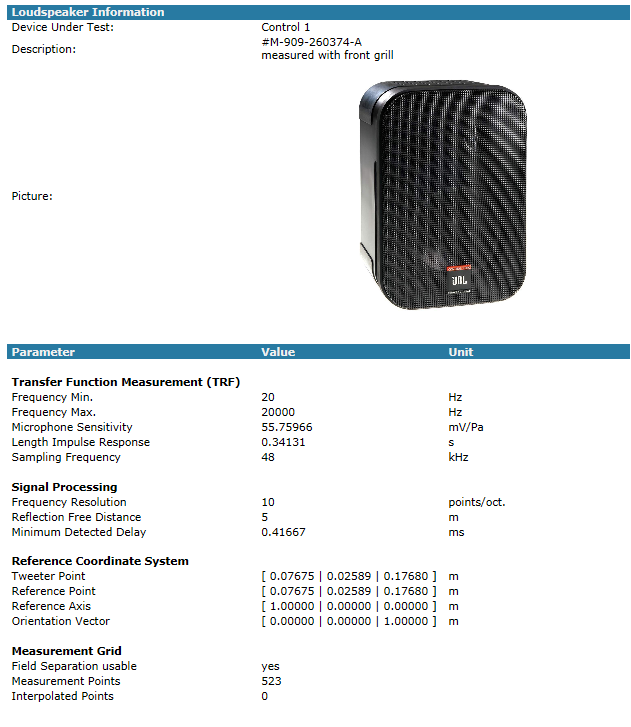
Loudspeaker Information#
In addition to the parameters and setting from the measure, further information about the loudspeaker can be added. For Example:
Name
Further description of the DUT
Picture of the DUT
The specified Loudspeaker Information are shown in the Summary result windows
Result Windows#
Summary Window#
After running the Measurement Data Container, the Summary window shows the content of the data container. This includes Loudspeaker Information, the measurement setup (e.g. microphone sensitivity, frequency range) as well parameters for further processing with the Holographic Field Identification (e.g. reference point, frequency resolution.)
Measurement Points#
The Measurement Points results windows visualizes the Reference Coordinate system and position of the Tweeter Point.
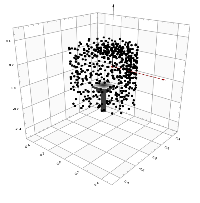
Activating Plot 3D Coordinates, the distribution of the measurement points is shown as well.
Holographic Field Identification#
How it works?#

At first all measured data is prepared for the further sound field analysis. This block executes standard signal processing operation like time windowing, fast Fourier transform, etc. In the next step, the processed data is committed to the holographic sound field identification, which solves the wave equation for the measured sound field. The results of the Holographic Field Identification are a set of holographic coefficients.
Operation Modes#
- Standard Field Identification
The Standard Field Identification uses a simple holographic model, which does not consider external sound sources. It expected an anechoic ambience. All disturbances from an imperfect measurement room can cause errors in the results.
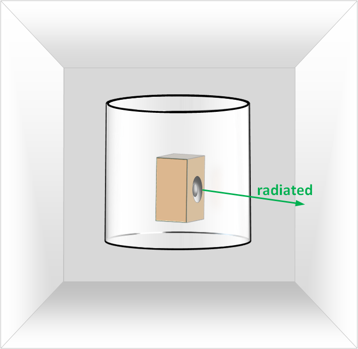
The standard field identification does not consider any room influences. That means, below the Reflection free frequency the measurement room have to be anechoic. Otherwise, the room effect causes inaccuracies in measurement results.
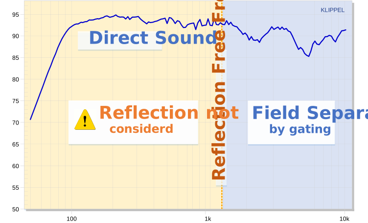
- Direct Sound Separation
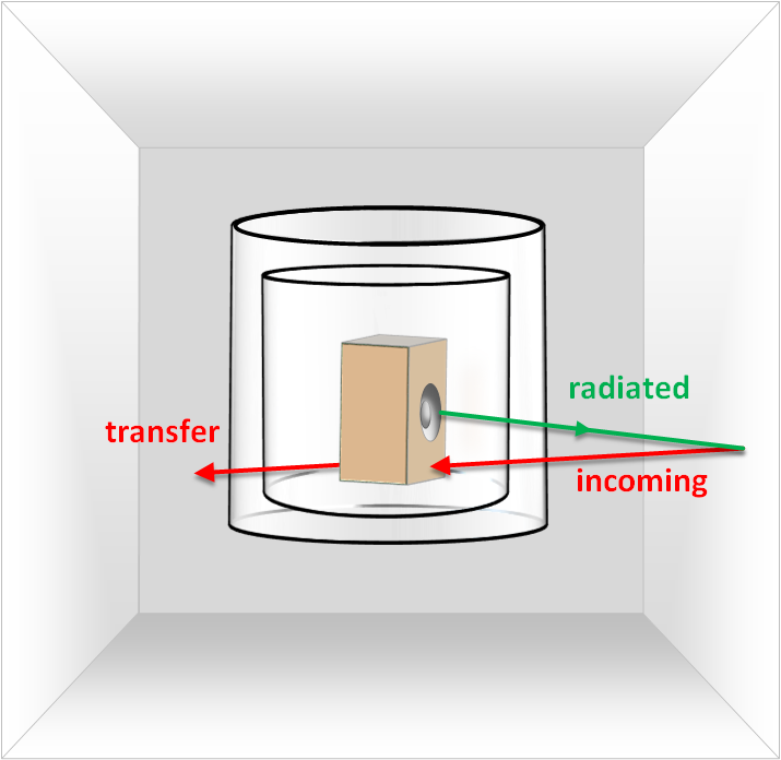
The direct sound separation considers external sound sources (e.g., reflections and room modes). By using a dual surface approach, the room effect can be separated from the direct sound of the device under test.
As seen in the picture the model detects the radiated sound of the DUT over the whole frequency band, using a combination of holographic modelling (low frequencies) and gating (high frequencies).
Standard Field Identification#
According to [1] the general solution of an exterior problem is:
\(p( r,\theta, \phi,\omega)\) : Complex sound pressure in Pa
\(C_{nm}(\omega)\) : Coefficients (Frequency dependent)
\(h_{n}(kr)\) : Hankel Functions (Radial functions)
\(Y_{n}^{m}( \theta,\phi )\) : Spherical Harmonics (Angular functions)
\(n,m\) : Indices of order and suborder
\(N\) : Order of Expansion
That means, the sound field of an arbitrary sound source can be characterized by a weighted sum of elementary sound sources. These elementary sources can be modeled by the product of spherical harmonics \(Y_{n}^{m}\) and hankel functions\(\ h_{n}\), which are solutions of the wave equation.
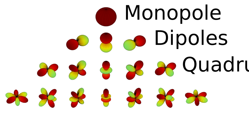
Using the phase definition, \(e^{- ikr}\) corresponds to an outgoing wave (an increase of the distance \(r\) causes a negative phase shift), the hankel function of the second kind \(h_{n}^{(2)}(kr)\) represents an outgoing wave. Thus, the solution of a sound field radiated from a sound source into free space is defined by:
Assuming that all sound sources are inside a minimum sphere with the radius \(a\), the coefficients \(C_{nm}\), which completely represent the sound field, are identified on this surface. Moreover, the sound pressure at each point outside the scanning surface can be extrapolated into free space.
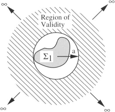
Direct Sound Separation#
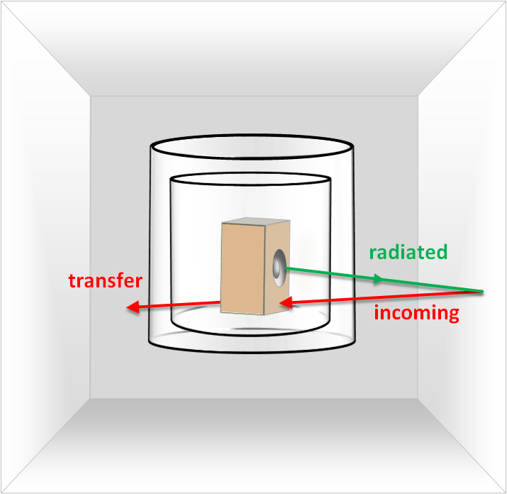
Measuring in non-anechoic condition is a challenging aspect. The near field measurement itself has some beneficial particularities. The direct sound dominates the total sound pressure, because it has a high level in comparison to the room reflections. Furthermore, the room reflections can be filtered out for high frequencies using time windowing. However, especially for low frequencies (below 1 kHz) the common windowing techniques are not applicable anymore. Also, room resonances appear which dominate the total sound pressure. Even in good anechoic rooms, room influence cannot be neglected below 100 Hz.
The Input-Output-Field Separation handles these problems by using an advanced holographic model. In addition to the primary sound source (DUT) secondary sound sources (reflections, room resonances) are considered.
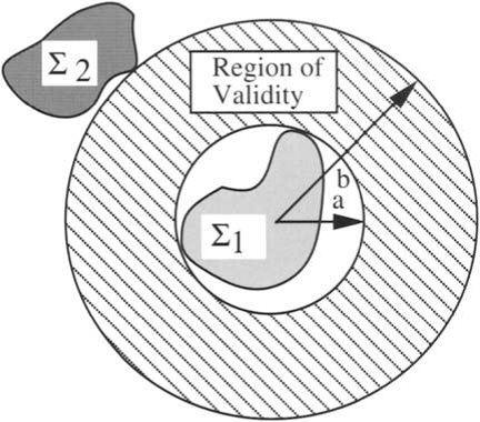
At each point of the region of validation the complex sound pressure is defined by the sum of outgoing and incoming waves.
Using the holographic approach, the total sound field can be characterized by:
This approach requires a scanning on two surfaces, which provides phase information. Thus, the direction of propagation of the sound waves can be identified and separated. Derived from the coefficients of the incoming and outgoing sound pressure, the radiated sound pressure of the DUT is determined on the measured surface and can be extrapolated into free space.
Configuration Check#
The Field identification starts with a configuration check. This includes the check parameters, limits and the measured grid.
Check Limits and Parameter#
This block checks the setting of the field identification. It includes a check of input parameters, check of mathematical limits like maximum theoretical order or singularity and check of physical limits like maximum available memory.
Check Measurement Grid#
Each order of spherical harmonics can produce a specific minimum beam width. Therefore, every order requires a minimum grid resolution. Is the grid resolution lower than the order requires, spatial aliasing effects may appear, which produces massive errors. In order to avoid these effects, the distribution of measurement points is analyzed in two steps which are described in the following.
Interpolating not accessible areas#
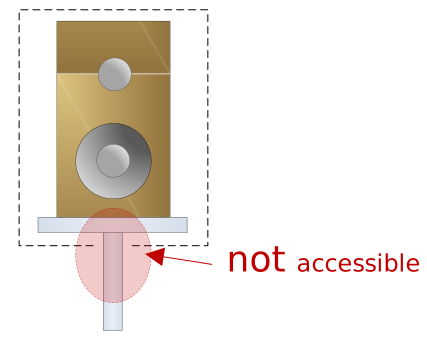
Caused by the mechanical setup of the NFS Hardware, there are areas which cannot be reached with the microphone. For example, the microphone cannot drive to all points of the bottom plane of the cylinder because of the speaker stand.
The holographic field identification needs a complete 3D surface around the sound source. In such a large area without points aliasing effect will appear. Spatial aliasing effects will limit the region of validity of the identified coefficients. That means in the region where these effect rises the coefficients are not valid anymore. Even a valid sound power calculation would not be possible anymore.
For these reasons, points are interpolated in this area by low order spherical harmonics. The interpolation is realized in three steps. At first the grid analyzed to detect the interpolation order dependent from the size of the interpolating area. Using the interpolation order the sound field is identified. At last, the free area is filled with points and the sound pressure is interpolated using the sound field extrapolation method.
The interpolation method produces just minor errors in the results of the sound field identification. The interpolated area the angle accuracy is limited because of the low order of spherical harmonics (spatial low pass). However, the interpolation method does not affect other radiation angles. Also, it has almost no influence to the sound power calculation.
Condition: The interpolated area in not in main radiation direction. It is supposed to be below the speaker (90° from on axis) or behind the speaker (180° from on-axis) where the SPL for high frequencies is < -20 dB comparing to the on-axis SPL.
Grid Resolution Check#
Even for well distributed measurement grid a critical order can be reached where grid resolution isn’t high enough for the spherical harmonics order. In that case also spatial aliasing effects will appear. For this reason, a protection algorithm is implemented which analyses the grid, calculates a maximum valid order and limits the order if necessary.
Signal Processing#

The raw measurement data (impulse responses) is filtered by a windowing function in time domain. The time window is calculated automatically, the user just specifies the target frequency resolution (Points Per Octave) and the covered distance of the first reflecting wave (Reflection Free Distance).
The next processing block is the Fast Fourier Transform (FFT) which transforms the windowed impulse response into frequency domain.
The last processing step is smoothing function. This block smoothed the transfer functions with the target frequency resolution. The frequency resolution is reduced to the target resolution as well.
Time Windowing#
The time windowing zeros out the impulse response in a chosen interval.
Using this technique, room reflections can be gated out for high frequencies. The standard signal processing operates with a dynamic windowing function, which calculated multiple time windows automatically.
At first the highest reflection free frequency \(f_{\text{rf}}\) is calculated directly from the reflection free distance \(d_{\text{rf}}\) and the target frequency resolution \(p_{\text{oct}}\). \((c\). speed of sound)
For all lower frequency bands, the length of window function is increased each octave dynamically dependent on the target frequency resolution. The window length is calculated by the following equation:
Each windowed time response is transformed into frequency domain and the complete frequency response is merged.
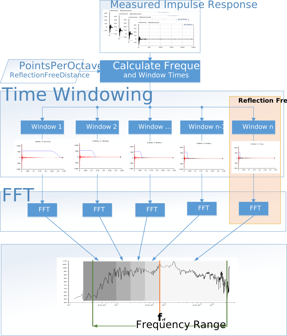
The Field Identification is using Tukey Windows defined by:
The parameter alpha modifies the shape of the window function from \(\alpha = 0\) (rectangular) to \(\alpha = 1\) (von Hann).
Smoothing#
For a better interpretation and increasing the SNR, the transfer function of each measurement point is smoothed. The smoothing is processed in the complex domain. That means real and imaginary part is smoothed separately. The bandwidth is defined by the parameter PointsPerOctave. The number frequency points is reduced to the target resolution as well.
Parameter#
- Data Container
Operation of the data container, from which the measured data is loaded
- Order of expansion
The order of expansions defines the number of terms of the series expansion. A sound field with a higher complexity needs more expansion terms and a higher order for the identification.
- Direct Sound Separation
Parameter to activate Field Separation for a non-anechoic scan.
☐ not checked: No room reflections are considered. (anechoic room)
☑ checked: Room reflection are considered
More details see Operation Modes
Symmetry Modes#
Parameter to activate a symmetry assumption in the Fitting and the Field Identification will only use subsets of spherical harmonics.
- No Symmetry
No symmetry is assumed and the sound field identification is performed with a complete set of basis function
- Baffle Symmetry
This symmetry is needed for half space measurements of transducers mounted in a baffle. The baffle is defined as a reflective plane at θ=90°, that causes a virtual mirror image of the sound field.
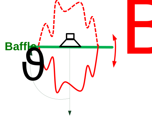
For Baffle Symmetry the sound field identification uses only spherical harmonics where n-m is an even number.
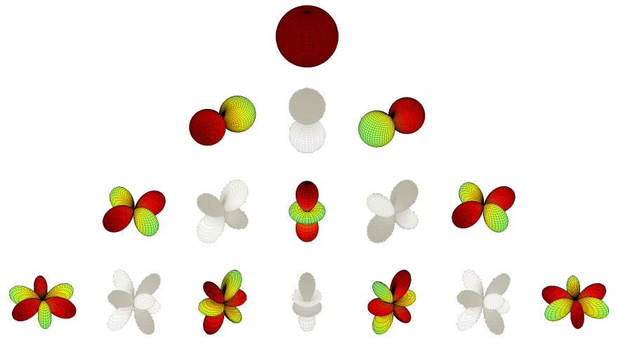
- Phi Symmetry (Single Plane)
Using phi symmetry, the spherical harmonics of m<0 are related to the spherical harmonics with m>0 by \(\mathbf{R}_{\mathbf{m}}\). This symmetry condition is considered for the sound field identification.
\[{R_m} = \frac{{{C_{mn}}}}{{{C_{ - mn}}}} = {\left( { - 1} \right)^{m + 1}}{\left( {\sin \left( {m{\phi _s}} \right) + i\cos \left( {m{\phi _s}} \right)} \right)^2}\]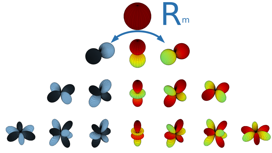
The Symmetry axis is defined by the angle \(\varphi_{\mathbf{S}}\). For Example:
Horizontal Symmetry (\(\varphi_{\mathbf{S}} = 0{^\circ}\))
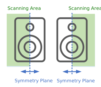
Vertical Symmetry (\(\varphi_{\mathbf{S}} = 90{^\circ}\))
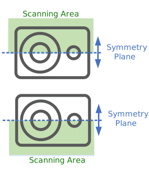
- Double Phi Symmetry (Dual Plane)
The double phi symmetry is using two orthogonal symmetry planes. This symmetry condition requires only a subset of spherical harmonics with even numbers of m.
The symmetry relation between positive and negative m is defined by:
\[{R_m} = \frac{{{C_{mn}}}}{{{C_{ - mn}}}} = {\left( { - 1} \right)^{m + 1}}{\left( {\sin \left( {m{\phi _s}} \right) + i\cos \left( {m{\phi _s}} \right)} \right)^2}\]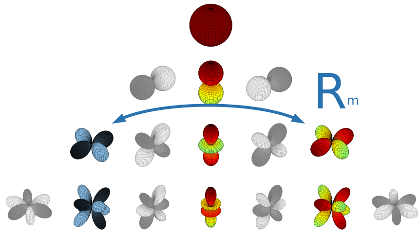
For Example, \(\varphi_{S} = 0\)° characterizes a vertical + horizontal orientation of the symmetry planes:
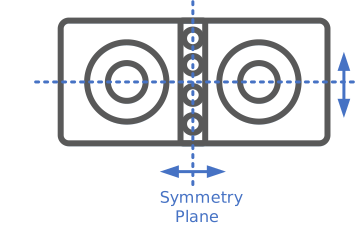
- Rotational
Rotational symmetry provides no variation of the sound field over the φ angle. This condition requires only the spherical harmonics of suborder m=0.
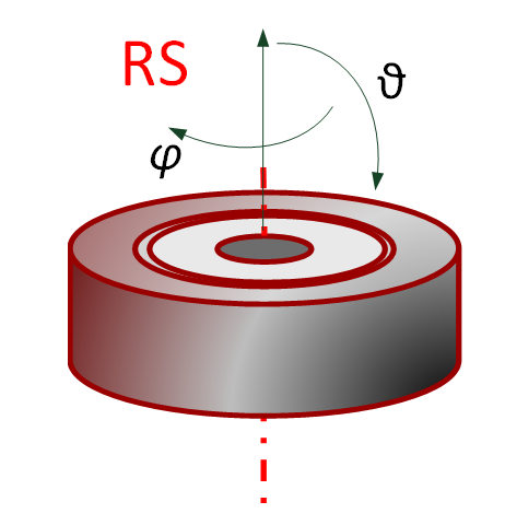
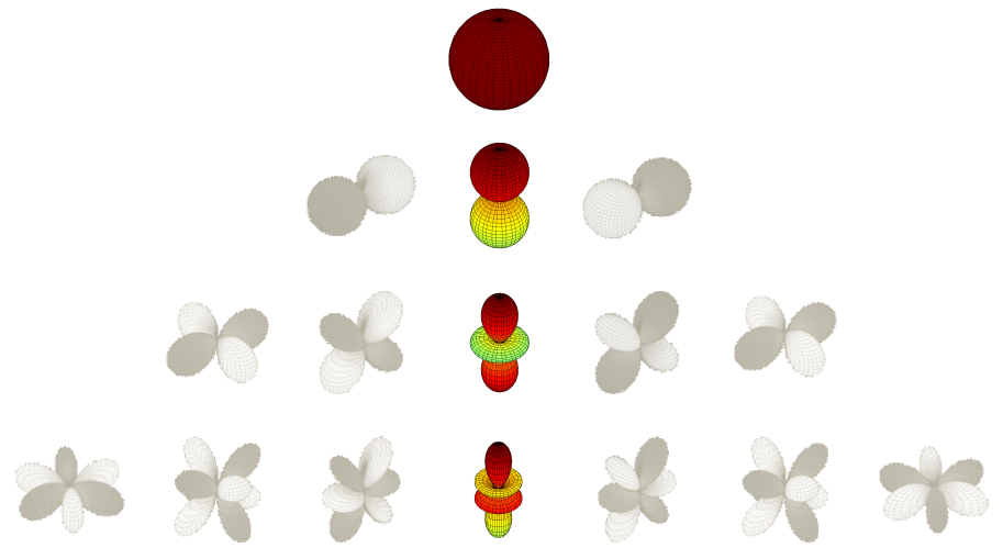
- Baffle + Phi Symmetry
Combination of baffle symmetry (θ=90°) and a single symmetry plane of φ.
- Baffle + Dual Phi Symmetry
Combination of baffle symmetry (θ=90°) and dual symmetry plane of φ.
- Baffle + Rotational Symmetry
Combination of baffle symmetry (θ=90°) and rotational Symmetry
- Baffle + Full Rotational Symmetry
Special symmetry mode for the SCN Near Field Add-On. This mode is using the rotational symmetric subset of spherical harmonics over the complete frequency band.
Symmetry + Direct Sound Separation#
Using direct sound separation not all symmetries can be applied to the full frequency band, because at low frequencies the room reflections are usually not matching the symmetry of the DUT. Thus, the following configurations will be used:
Mode |
Low Frequencies (DSS) |
High Frequencies (Windowed) |
|---|---|---|
Phi Symmetry |
No Symmetry |
Phi Symmetry |
Double Phi Symmetry |
No Symmetry |
Double Phi Symmetry |
Rotational |
No Symmetry |
Rotational |
Baffle + Phi Symmetry |
Baffle Symmetry |
Baffle + Phi Symmetry |
Baffle + Double Phi Symmetry |
Baffle Symmetry |
Baffle + Double Phi Symmetry |
Baffle + Rotational |
Baffle Symmetry |
Baffle + Rotational |
Baffle + Full Rotational |
Baffle + Rotational |
Baffle + Rotational |
- Results Frequency Spacing
Spacing of the frequency points of the exported data - resolutions higher than the target frequency resolution, which is specified by the window length are generated by zero padding.
- Resolution
Frequency points per octave of the exported data
- Improved Off-Axis Interpolation
For very directive speakers (e.g., Line Arrays with multiple horns), the standard interpolation method (More details see Signal Processing) may cause unexpected side lobes in the area of the interpolation. To avoid these effects, there is an alternative interpolation that is optimized for DUTs with high beaming.
- Speed of sound
Sonic speed in m/s that is used for the calculations.
- SPL Response Point - Display
The display parameter selects the measurement point that is shown in the H(f) Transfer Function Magnitude Window
- Frequency Apparent Power – Display
The display parameter selects which frequency is shown in the apparent sound power from distance window
Results#
Summary Window#
The Summary window shows important parameter and results of the operation. Furthermore, it propagates warnings and errors.
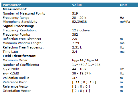
Fitting Error#
The fitting error is an indicator of the accuracy of the sound field identification. It shows how well the identified sound pressure corresponds with the measured sound pressure. It is calculated over all measured points and is defined by:
The window visualizes the frequency dependent fitting error in dB [ \(\ E_{\text{Fit}}/dB = 10\ log\left( \frac{e_{\text{fit}}}{100\%} \right)\)]. In general, the fitting error is supposed be to less than -20 dB (1 % error) in the pass band of the DUT.
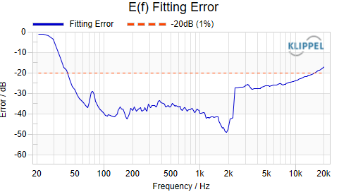
As seen in the example data the field identification is done with a sufficient order because the fitting error is below -20 dB in almost the full audio band. Only for very low frequencies the fitting error rises above -10 dB. This increase is uncritical because it is out of the working range of the loudspeaker. In this frequency band the SNR of the measurement is very low and the error is caused by noise. To get this information it is always important to check the other measures to rate the fitting error.
Order of Expansions#
This window visualizes configuration of the order of expansion dependent from frequency. As seen in the picture, the order increases dynamically with the frequency.
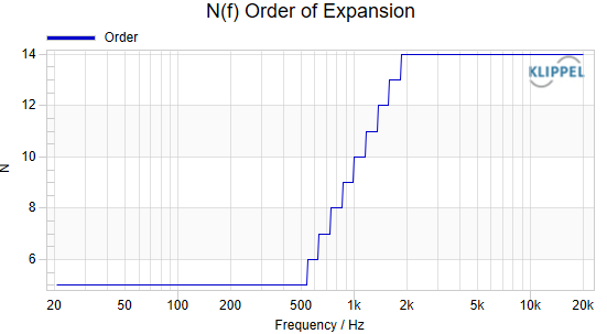
The order can be limited for multiple reasons (e.g. numerical reason, spatial aliasing, number of points). If one of the limits is exceeded, it will be visualized in the result window.
Radiated Sound Power#
The sound power radiated by specific order spherical harmonics is a measure, to determine the complexity of a sound source. The plot shows the total sound power radiated to the far field for each frequency. The radiated sound power of each spherical harmonics order is shown as well. Thus, the dominant orders for each frequency can be easily detected.
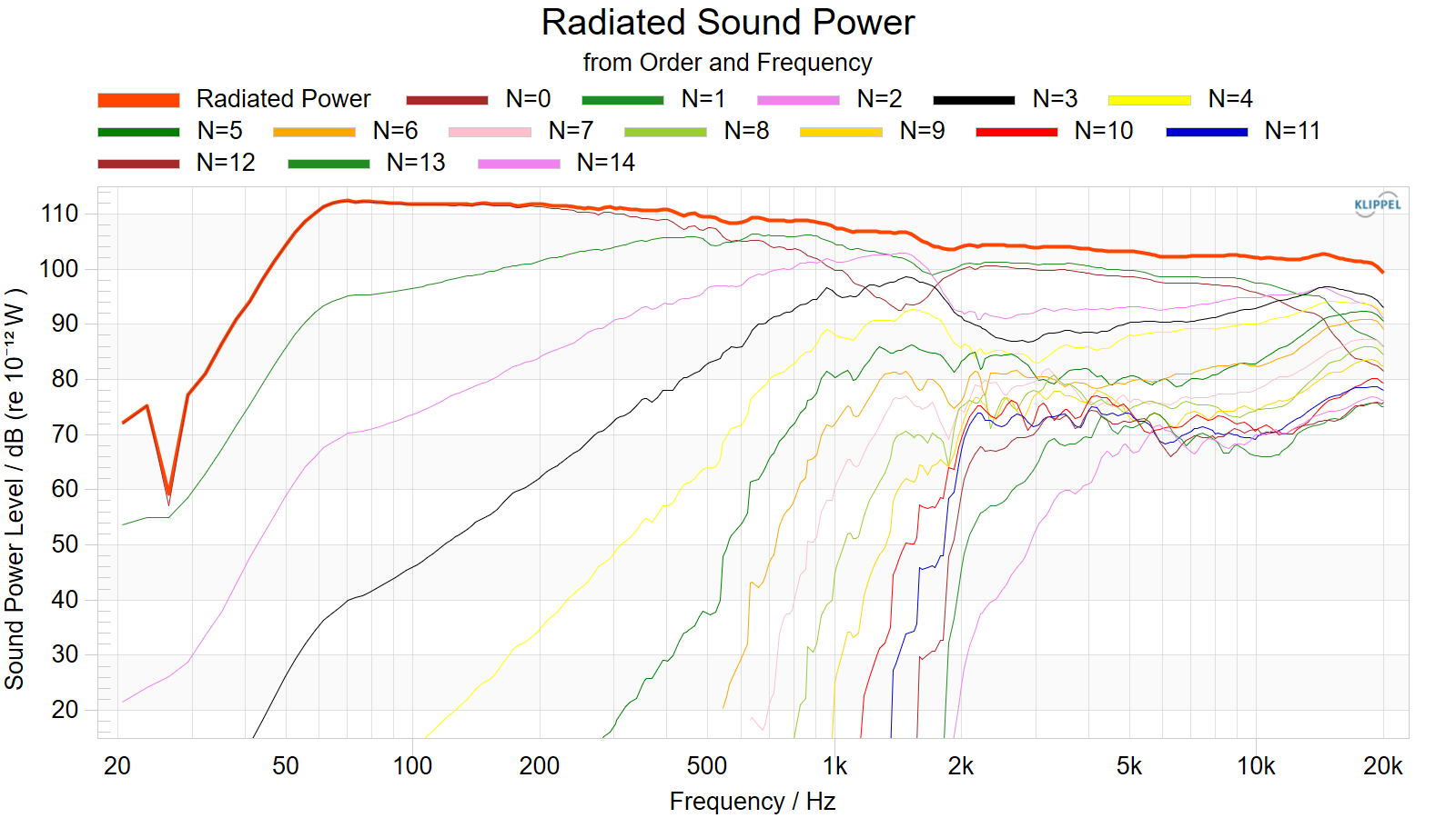
As seen in the picture for low frequencies the lower order spherical harmonics (Monopole N = 0 / Dipole N = 1) are dominant. With rising frequency the power of the higher orders increases, because the sound field becomes more complex.
Apparent Sound Power#
The graph of the power from distance visualizes the power transfer from the near field to the far field. The near field is characterized by a high amount of reactive power represented by high order Hankel functions. As seen in the plot, the near field effects decrease with the distance. In the far field, the sound power is constant over distance because velocity and sound pressure are in phase.
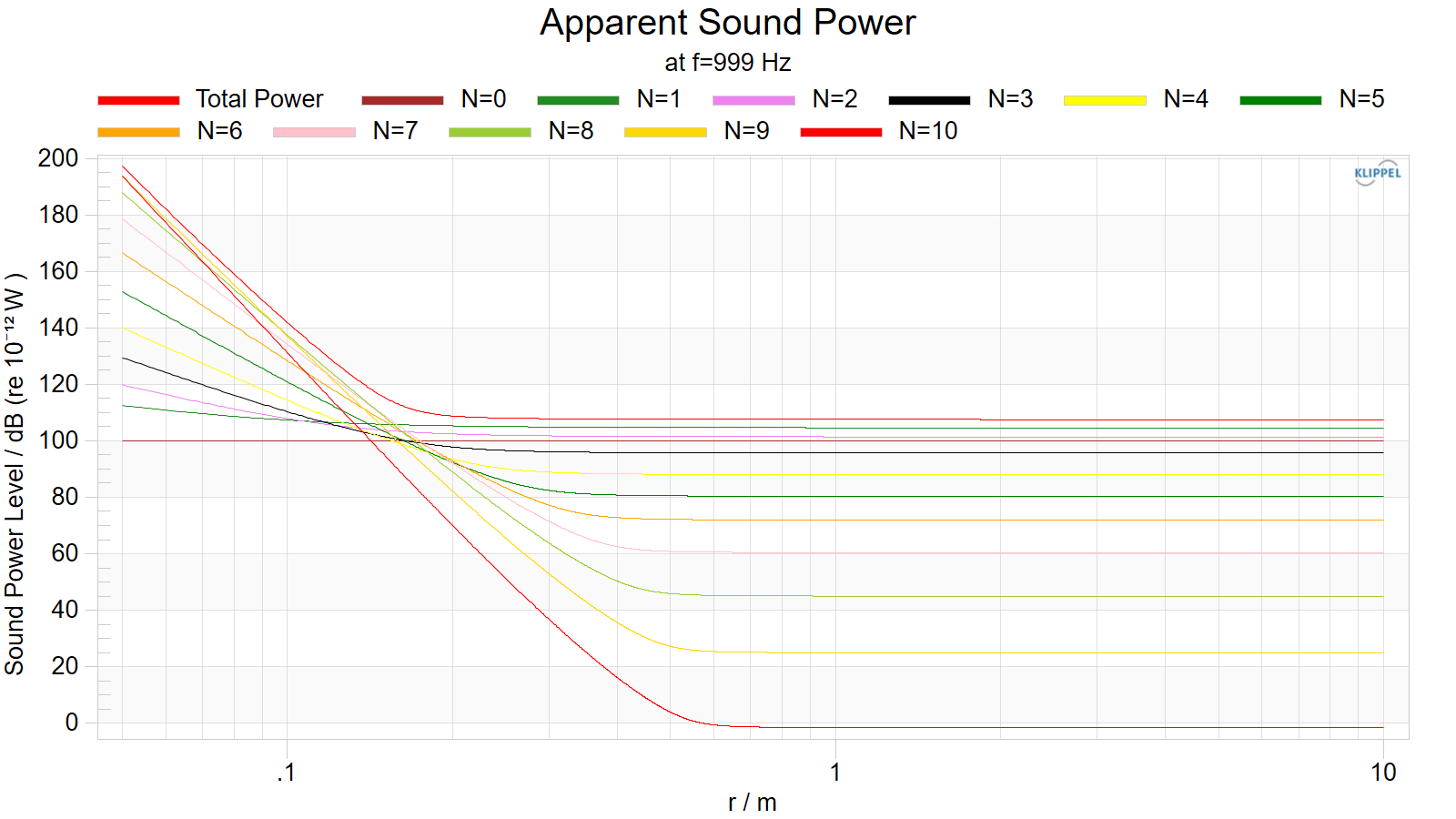
Near Field Response#
This Results window shows the comparison of the identified transfer function and the measured transfer function of one measurement point. For low frequencies the Input-Output Field Separation is activated which splits the measured sound field into radiated wave (blue solid line) and secondary sound wave (blue dashed line). For high frequency above the reflection free frequency the separation can be done by time windowing.
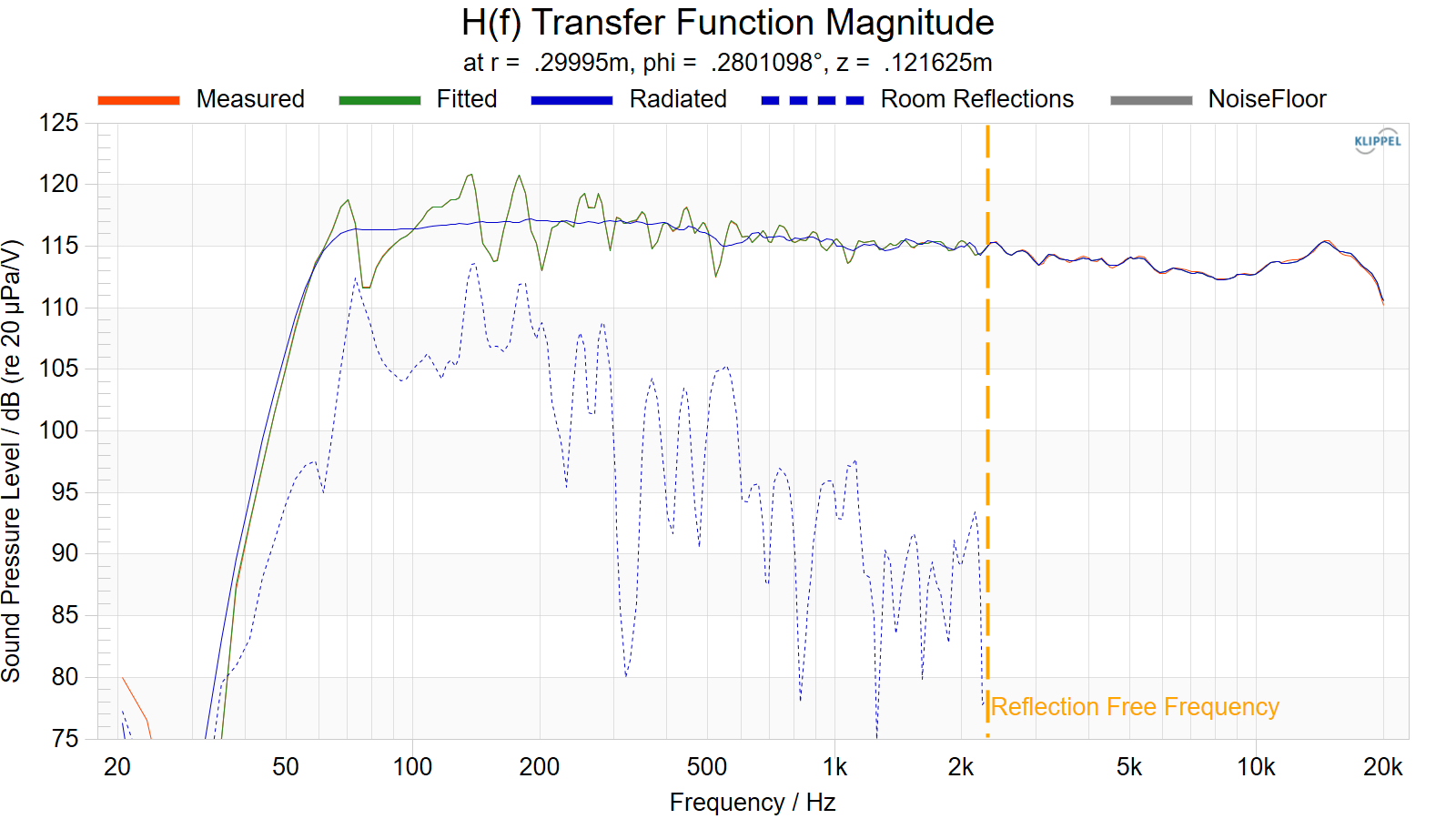
Handle this measure with care because it is just at a single measurement point and is not a global measure. However, this window can be useful to see basic properties of the DUT, like the working range or SNR and help to rate the fitting error.
Impulse Response#
The Impulse Response window shows the measured impulse response of a measured point. The applied window functions are plotted in the window as well.
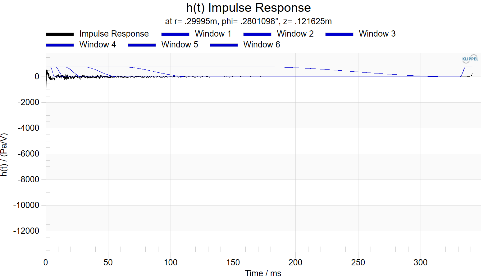
Measurement Points#
The distribution of measurement points can be easily checked using the measurement point window. It visualizes the point distribution over the radiation angles phi and theta.
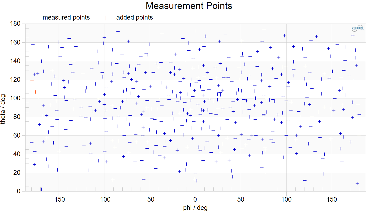
Symmetry Factors#
The Symmetry Factor S window describe how symmetric the sound field is based on the spherical harmonic coefficients. It’s defined by the sound power of the symmetrical part related to the total sound power.
A symmetry factor of 1 means that the sound field fulfills the symmetry condition by 100%.
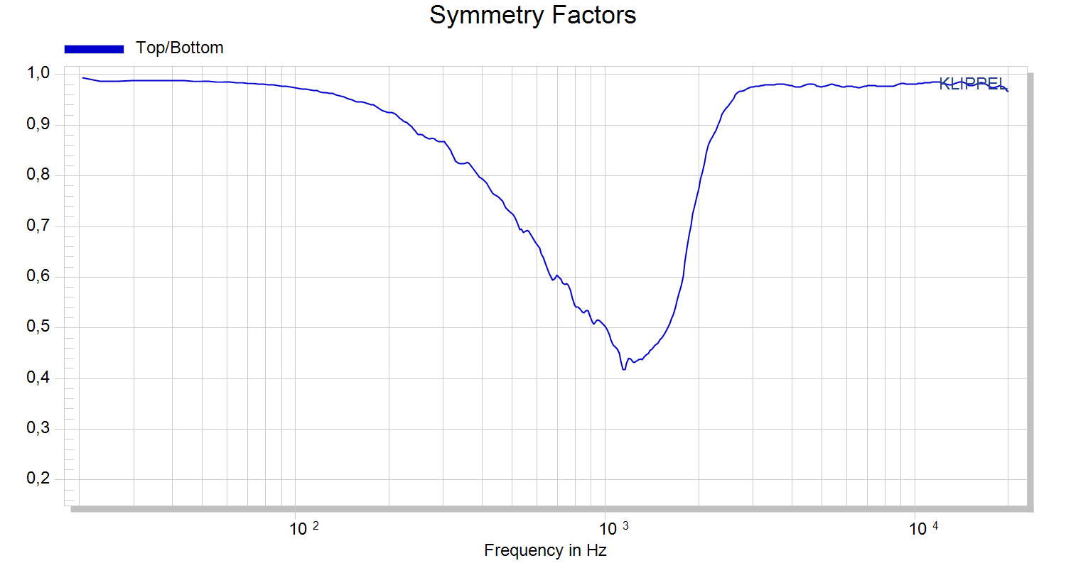
Symmetry Sound Power#
The Symmetry Sound Power shows the decomposition of the symmetric and asymmetric part of the total sound power. In following example, the sound field is very symmetrical at low and high frequencies. In this range the sound power is dominated by symmetrical part and the asymmetric part is -20 dB below. Between 500 Hz and 2 kHz at the crossover the asymmetric part is producing the same amount of sound power which indicates an asymmetric sound field.
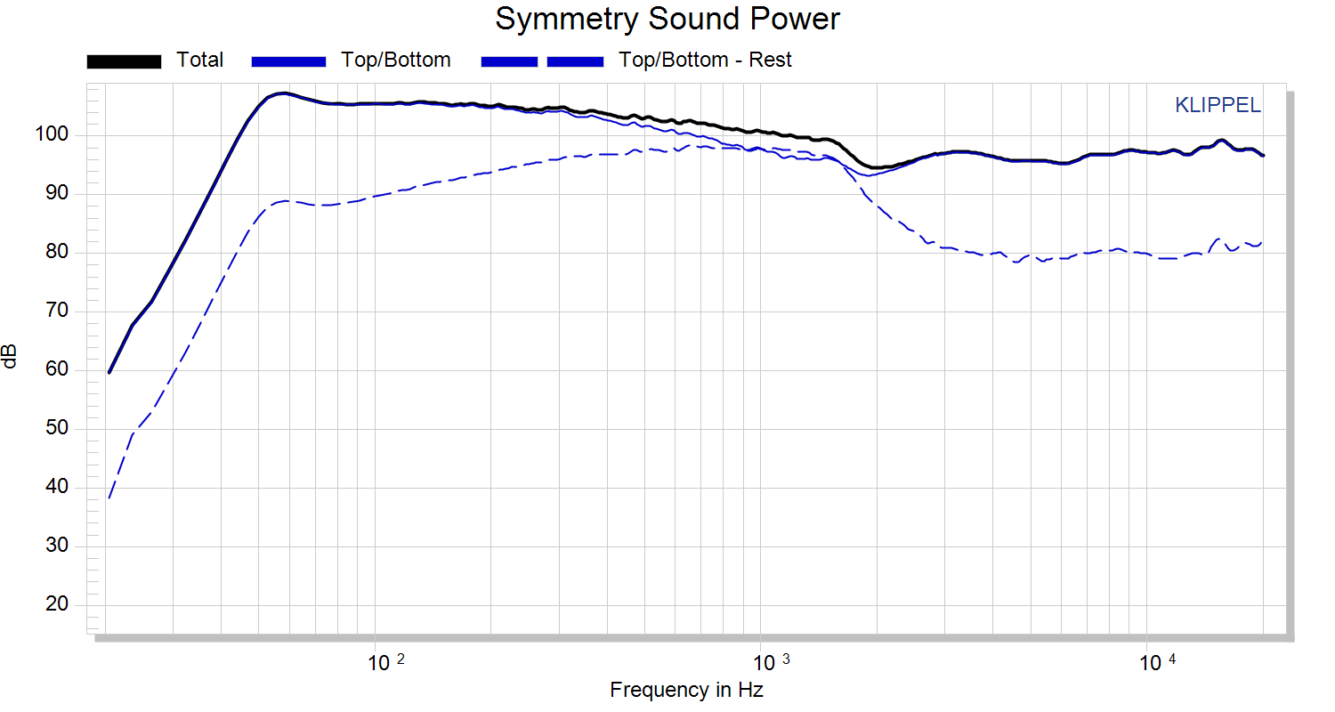
Visualization#
Parameter#
Input#
- Input Data Format
Visualization can analyze measurement data from a Near Field Scanner Measurement (NFS) as well as data measured with a traditional Polar Far Field Measurement (POL)
For both, NFS and POL, the visualization module will generate a set of far field characteristics. (e.g., Contour Plot, Polar Plot, Directivity Balloon, etc.)
In addition, the Visualization of NFS data will provide more feature like an Export Interface and a Near Field Analysis. Also, the far field characteristics can be calculated at any distance outside the scanning surface including an exact model of near field effects.
- Device Under Test
Selection of microphone or loudspeaker visualization for Polar Far Field Measurement (POL)
For each mode specific measures are calculated e.g.
For microphones: free-field and diffuse-filed sensitivity
For loudspeakers: sound power, impulse response, group delay
- Input Type
Analyzing NFS data the sound field can be either visualized for a single measurement or a multi-source measurement. (For more details see Multisource Super Positioning)
- Nominal Impedance
Nominal Impedance of the loudspeaker.
Using the data export the impedance curve is converted and export Using the CLF-Export the nominal impedance will be included in the *.tab-file
- Impedance Z(f)
Electrical Impedance curve Z(f) of the loudspeaker.
The complex data export module includes the impedance curve for certain formats. The impedance data is available in the following formats:
EASE: Saved as a .txt file (CLIO Frequency Files format) in the export folder. This can be imported into EASE SpeakerLab’s Source Editor under Properties.
CLF: Included in the .tab file, along with the nominal impedance (if specified).
- Global Reference System
Parameter to activate a manual definition of the Reference Coordinate System related to the NFS Coordinate System.
If parameter is unchecked the Reference Point, Reference Axis and Orientation Vector are automatically imported from the Field Identification operation.
Data Comparison#
For an easier comparison of different measurements, the NFS Visualization can import two set of holographic coefficients and visualize them simultaneously. In this mode all 2D graphs are showing curves for each speaker and all 3D and color graphs are doubled.
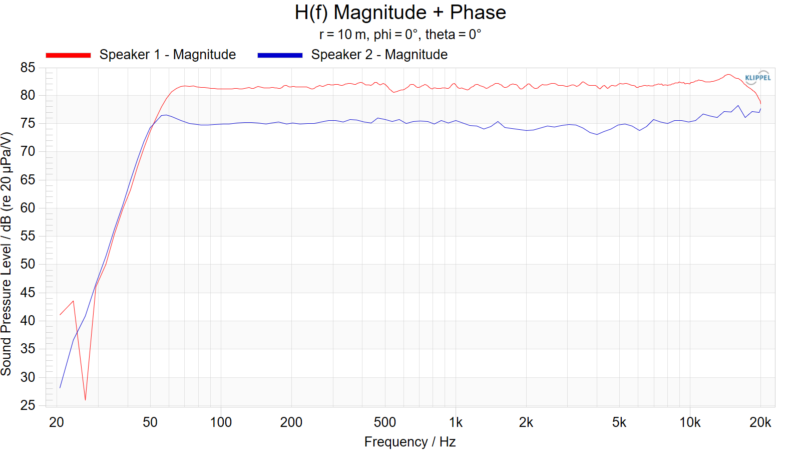
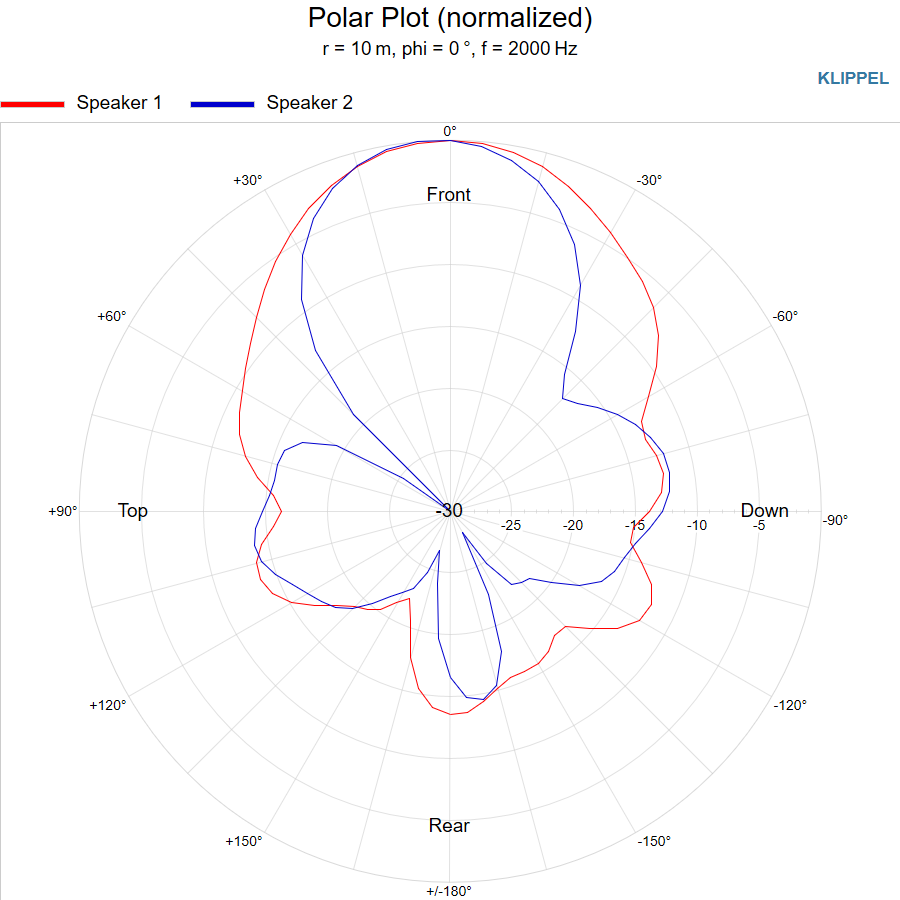
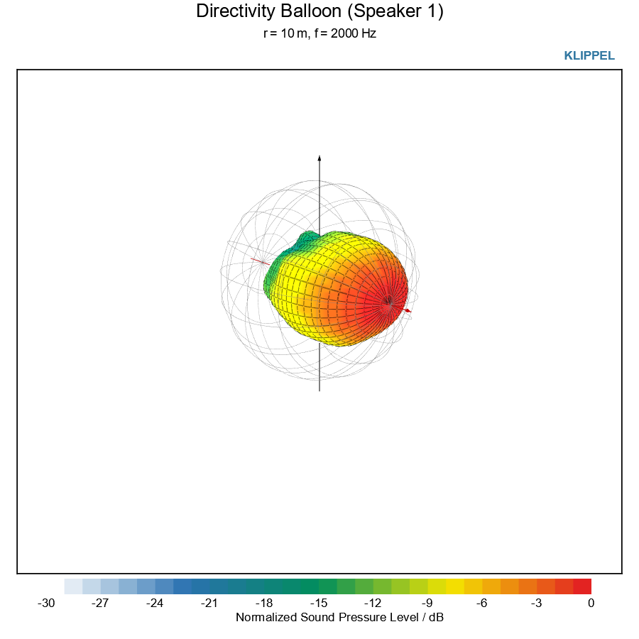
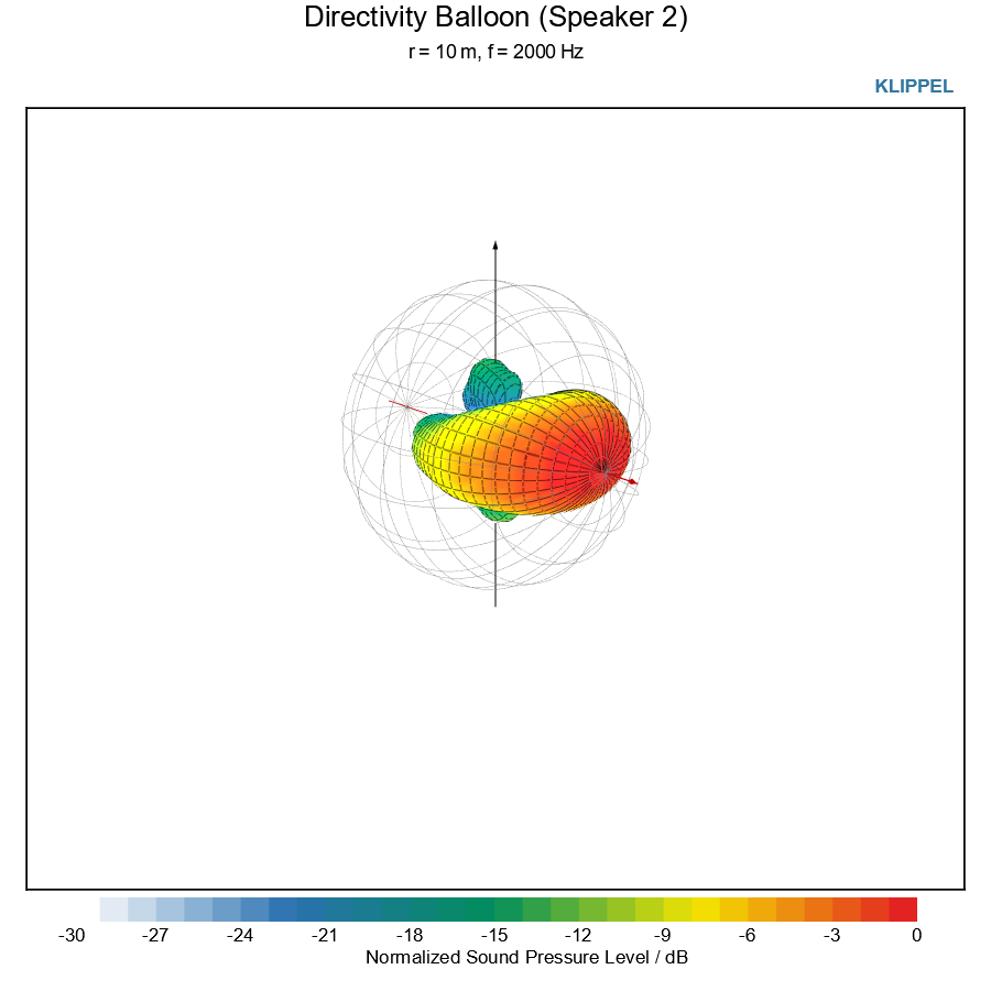
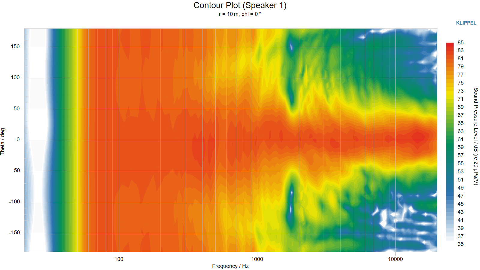
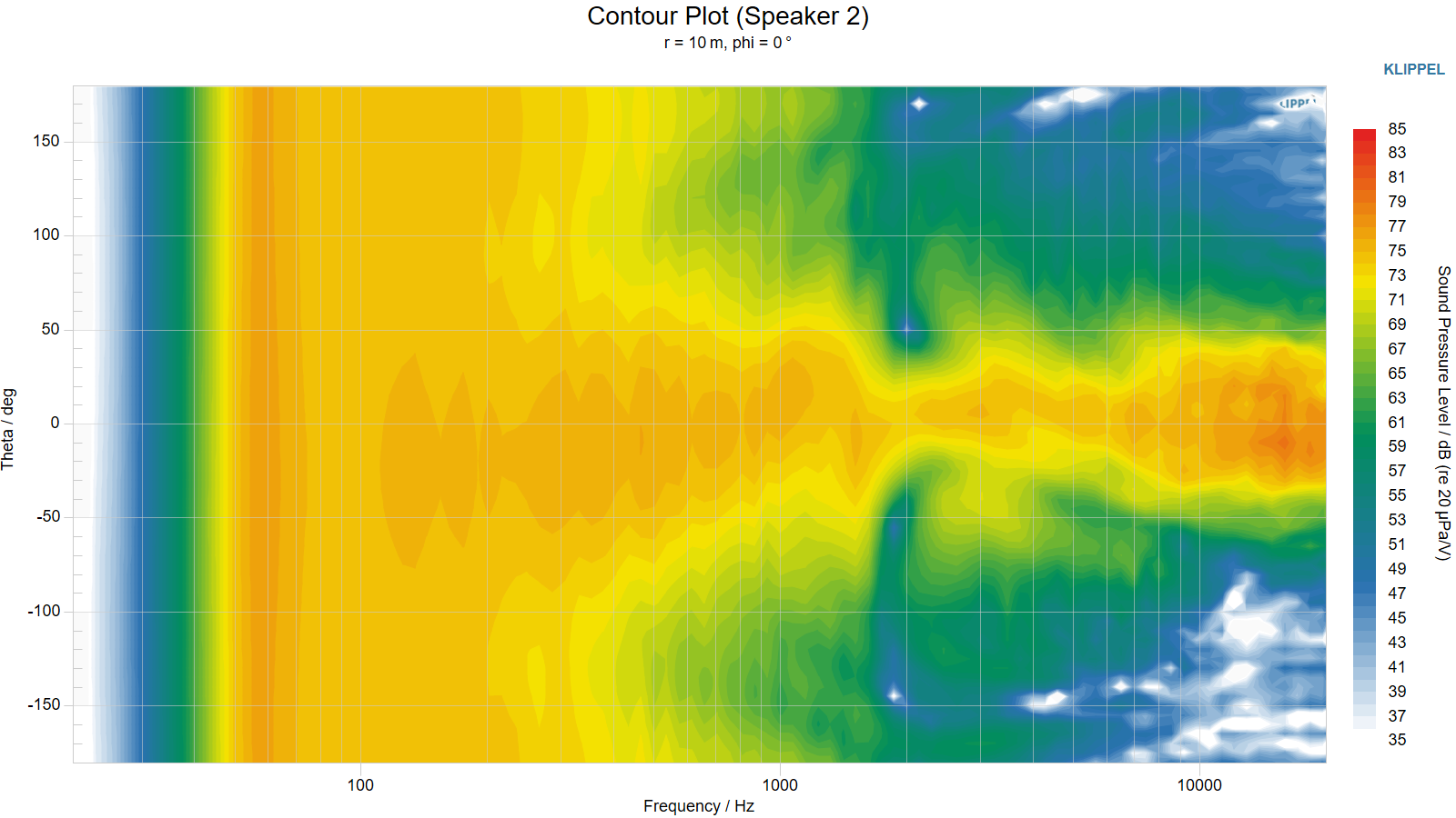
Multisource Super Positioning#
When measuring large sound sources with multiple speakers (e.g., line arrays, sound bars) it is recommended to measure the speakers separately and superposition the individual measurements in the software. For this application, data from multiple measurements can be loaded into the software and can be freely positioned in 3D Space. During the plot calculation the individual sound sources are superimposed to generate the total sound pressure output of audio device.
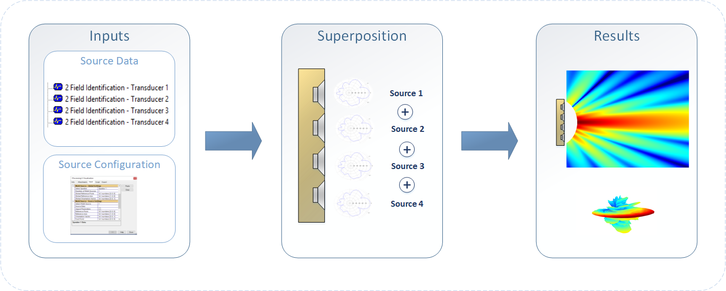
- Number of Sources
The Parameter defines the number of multi-sources, which are super positioned.
- Select Source
Parameter to select the source that should be configured.
- Source Data
Name of the Field Identification operation, from which the source data is loaded.
- Import Parameters
If checked the reference coordinates system is automatically imported from the selected the Field Identification module.
- Reference Point
Position of the Reference Point of the selected sound source relative to the Foot Point. Cartesian coordinates [x; y; z ].
- Reference Axis
The Reference Axis specifies the main direction of the sound radiation and is identical to theta=0° axis. It has to be a column vector with three Cartesian coordinates [x; y; z ].
- Orientation Vector
The Orientation Vector specifies the orientation of the sound source and is identical to phi=0° axis. Usually, it points to the top of the DUT. Cartesian coordinates [x; y; z].
- Foot Point
Position of the origin of the sound source. Parameter can be used to shift the source position in 3D space. Cartesian coordinates [x; y; z ].
- Display Style
Selection of the visualization style of the sound source in the Multi Source Configuration Window
No (displays only reference coodinates systems)
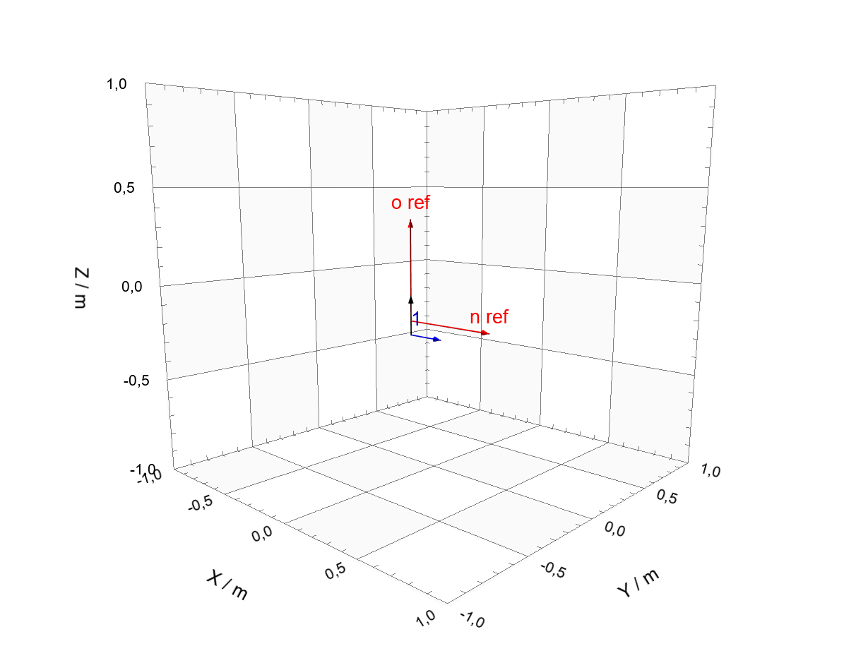
Cabinet + Driver (filled)
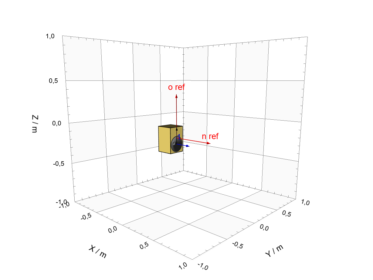
Cabinet + Driver (line)
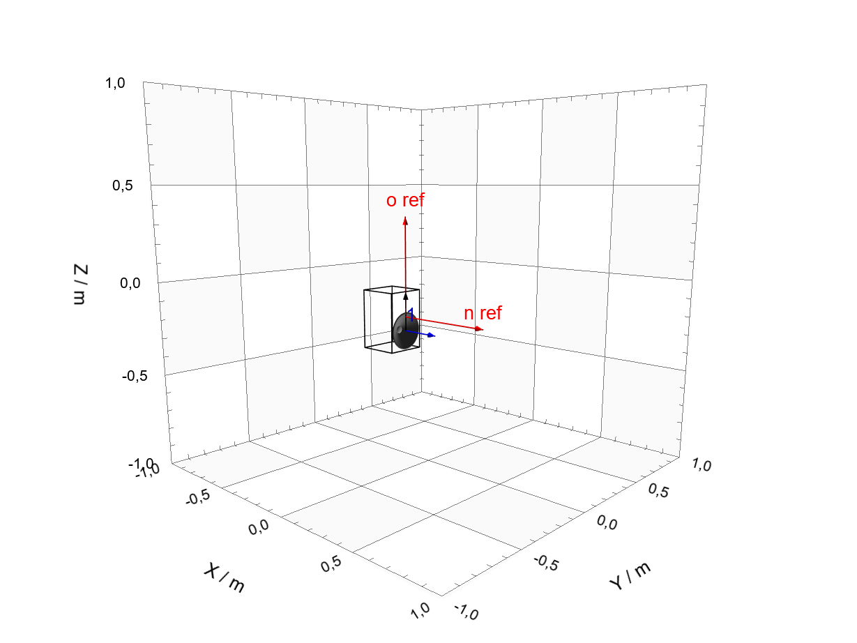
Driver
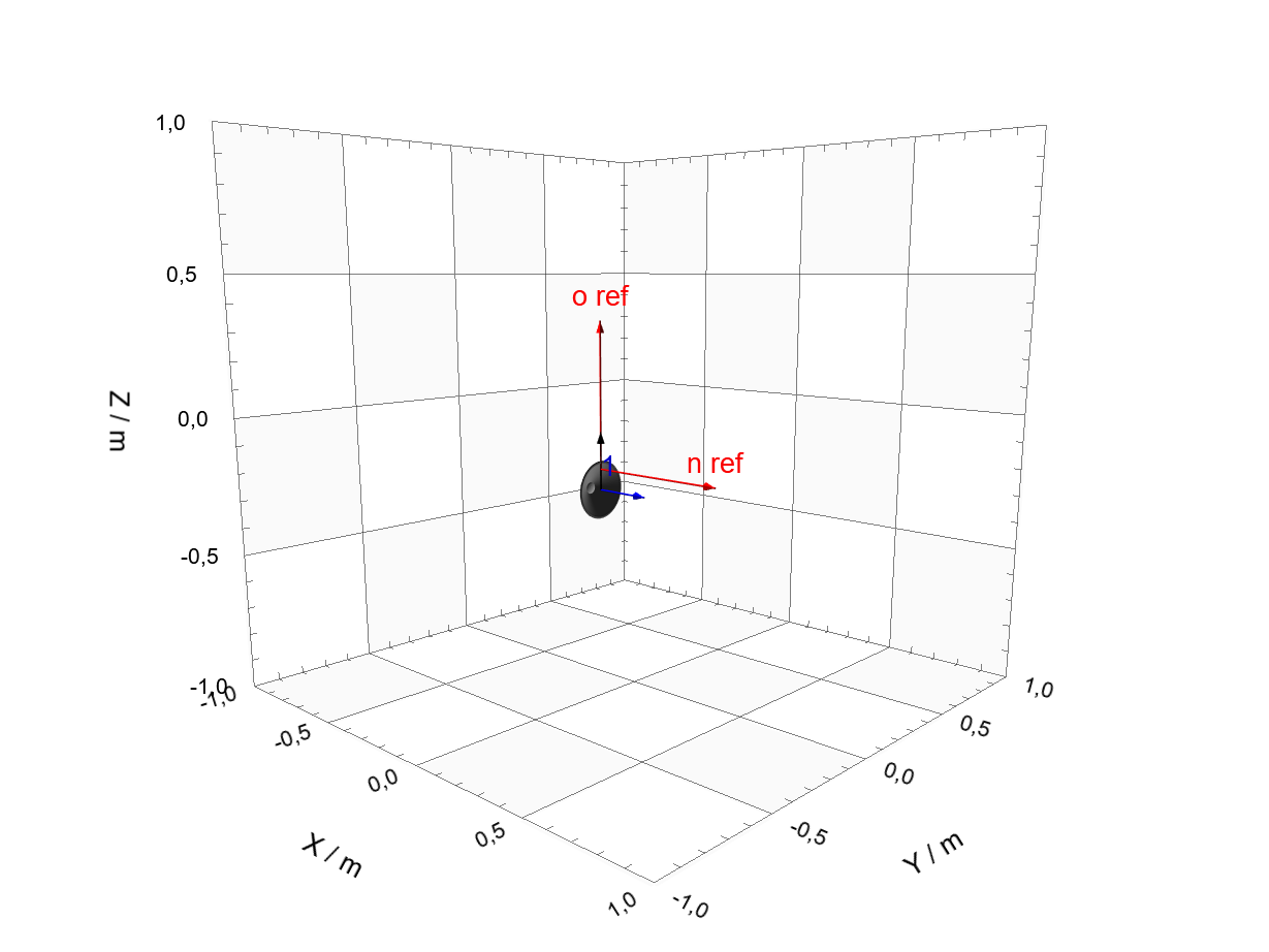
- Cabinet Information
Definiton of the loudspeaker size displayed in the Multi Source Configuration Window
Format 1: Symmetric cabinet with the Reference Point in the center
height
width
depth

Format 2: Asymmetric cabinet with minimum and maximum related to the Reference Point.
min. height | max. height
min. width  | max. width
min. depth  | max. depth

- Diameter of Transducer
\(\text{m}\) Definition of driver diameter displayed in the Multi Source Configuration Window
- Add Filter
For additional simulations, (e.g., crossover, or beam steering) a filter curve can be added to each sound source. I can be either a Magnitude Response [Frequency in Hz | Magnitude in dB] or a transfer function with magnitude and phase.
Format:
column1          |  column2          |   column3
Frequency in Hz  |  Magnitude in dB  |   Phase in Degree
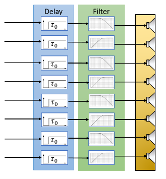
- Add Delay
Using this parameter, a constant time delay can be added to the selected sound source.
Processing#
- Half Space Measurement / Baffle
☑ checked: Characteristics are visualized from -90°≤ θ ≤ 90°
☐ not checked: Characteristics are visualized from -180°≤ θ ≤ 180°
- Speed of Sound
To analyze the sound field under target conditions, the speed of sound can be set manually. [Default Value: 343m/s]
Near Field Analysis#
Calculation Mode#
Parameter to activate the Near Field Visualization
Projection Surface - Configuration#
- Surface
- Selection of the shape of the projection surface. Available options:Cube
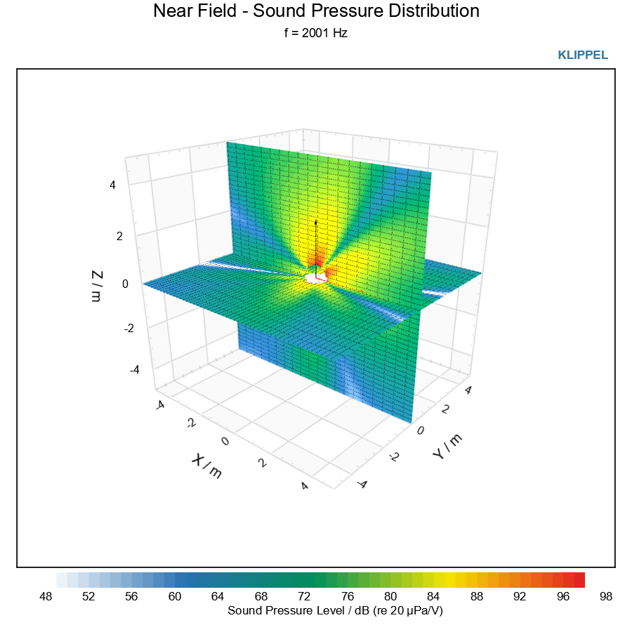 Sphere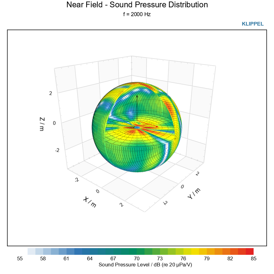
- X-Center Point
- \(\text{m}\)Center position of the projection surface (X-coordinate)
- Y-Center Point
- \(\text{m}\)Center position of the projection surface (Y-coordinate)
- Z-Center Point
- \(\text{m}\)Center position of the projection surface (Z-coordinate)
- Size
- \(\text{m}\)Size of the projection planes
- Resolution (Cube)
- \(\text{m}\)Mesh Resolution of the projection plane
- Angular Resolution (Sphere)
- \(\text{°}\)Angular resolution of the spherical projection plane
- Radius Resolution (Sphere)
- \(\text{m}\)Radius increments of the spherical projection plane
- Frequency
- \(\text{Hz}\)Calculation frequency of the near field sound pressure distribution
Projection Surface - Display#
Display Parameter of the sound pressure distribution result window.
- Color Data
- Defines which measure the surface color is visualizing. The following option can be selected:- Sound Pressure Level
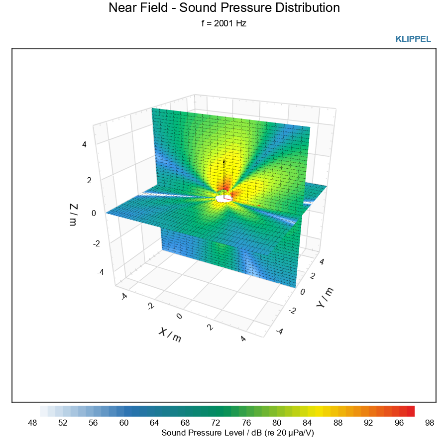 - Phase
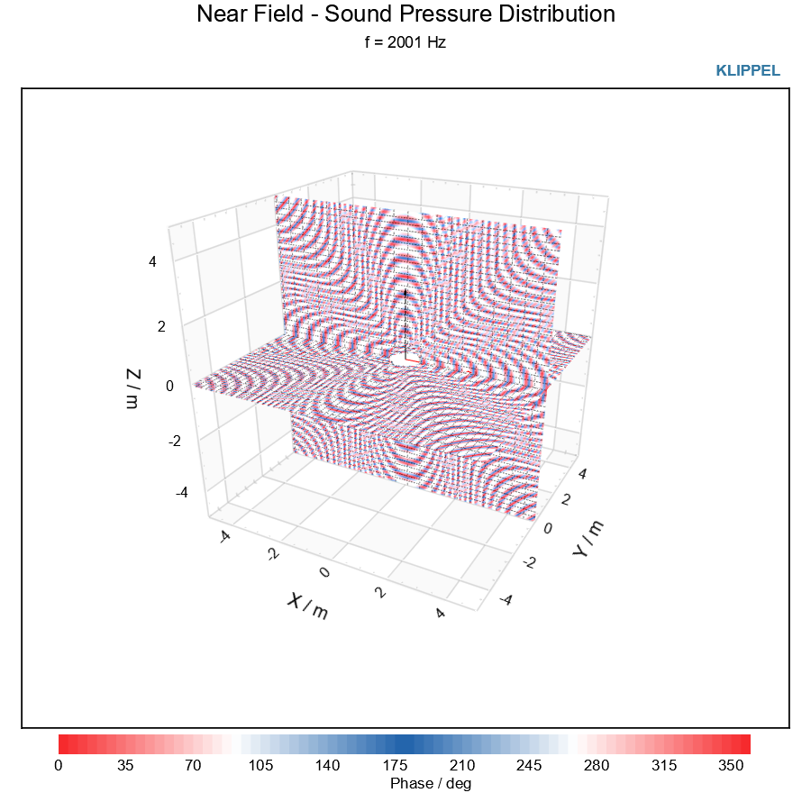 - Sound wave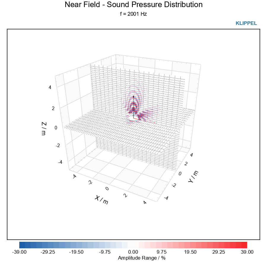
- Normalize (SPL)
- If checked the sound pressure distribution plot is normalized to the maximum SPL
- Display Range (SPL)
- \(\text{dB}\)Range of the SPL colormap
- Colormap (SPL)
- Selection of the color map for the sound pressure
- Color step size (SPL)
- \(\text{dB}\)Step size of the SPL colormap
- Color Range (Sound Wave)
\(\text{%}\) The sound wave plot visualizes the amplitude and phase combined and is displayed linear. Using the Color Range parameter, the amplitude value of the plot can be compressed.
100%: Original Amplitude (full dynamic)
0%: no amplitude information (only phase)
- Show/Hide Planes
- Check boxes to show and hide planes or segments of the spherical surface
Listening Points - Configuration#
To analyze the sound pressure frequency response in the near field of a loudspeaker, listening points can be set at any position. This can be used to investigate a target listening zone which can be for example a plane, a sphere or a cubical.
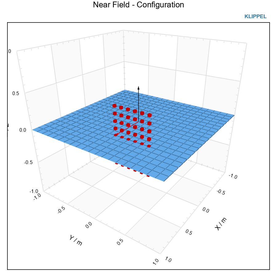
- Coordinate System
- Selects in which coordinate system the listening points are be defined. It can be either the physical coordinate system of the Near Field Scanner or the Reference Coordinate System which is defined by Reference Point, Reference Axis and Orientation Vector.
- Type
Type of the coordinate definition. The coordinates can be defined in the common coordinate formats:
Cartesian (X,Y,Z)
Cylindrical (R, Phi, Z)
Spherical (R, Phi, Theta)
- Coordinates
- List of coordinates of the Listening Points.
Listening Points - Display#
- Display Range SPL
- \(\text{dB}\)Parameter defines the display range of the sound pressure level. If unchecked minimum and maximum is set automatically
- Show Phase
- Show or hide the phase response
- Unwrap phase
- Switch between a wrapped or continuous Phase
- Remove Time Delay
\(\text{ms}\)
Parameter to remove a fixed delay from the phase responses. The following options are available:
Automatic (based on mean group delay)
Distance to Reference Point (propagation delay of the sound wave)
Custom (User defined delay in ms)
- Reference Voltage
\(\text{V}\)
Linear scaling to a defined input voltage. If unchecked response is referenced to 1Vrms
- Result Frequencies
Selection of the displayed frequencies. This can be:
Original (calculated Frequencies of Field Identification)
ISO Frequencies (e.g. R10, R80)
by Resolution (User Defined Resolution in Points per octave)
Custom (User Defined Frequencies)
- Frequency Resolution
\(\text{pts./oct.}\)
Frequency resolution for Result Frequencies setting: by Resolution.
- Custom Frequencies
\(\text{Hz}\)
Table of custom frequencies for Result Frequencies setting: Custom
- Smoothing
\(\text{pts./oct.}\)
Parameter to apply smoothing to the transfer functions.
Far Field Characteristics#
The far field characteristics are visualizing the sound field of a loudspeaker projected on a spherical surface with r (radius), θ (polar angle) and φ (circular angle). According to IEC 60268-21 the position of the spherical coordinate system is defined by the Reference Axis nref at θ=0°and the Orientation Vector oref at φ=0°.
- Calculation Mode
The Visualization can calculate the far field in the following modes:
Off: Nothing is calculated. This option is useful to save calculation time, for example when the visualization operation is only used for near field analysis.
Complete Calculation: In this mode the visualization will run a complete initial calculation that generates a full set of far field data for the defined radius and the defined angular resolution. After this initial calculation, most visualization settings can be modified interactively (e.g., theta, phi, frequency, etc.) without the need for further time-consuming calculations, because the data is loaded from this stored data set.
Fast Calculation: When only a subset of far field characteristics is required, the fast calculation mode can be used. In this mode only the selected plots will be calculated, which is usually much faster than a complete calculation. However, in the further analysis the module is less interactive and parameter modifications may require a recalculation.
- Radius
\(r\) in \(\text{m}\)
The radius specifies the distance to reference point of all far field characteristics.
When analyzing NFS data this can be any radius larger than the minimum sphere, which is defined by the size of the measurement surface.
For POL measurement this radius is fixed and defined by the measurement distance.
- Resolution
\(\Delta \varphi\), \(\Delta \vartheta\) in \(\text{°}\)
Angular resolution of theta and phi for all far field visualizations.
This Parameter is only relevant for NFS data, for which the angular resolution of the results can be defined freely.
For POL the resolution it is defined directly by the measurement points.
- Theta
\(\vartheta\) in \(\text{°}\)
Selection of the polar angle theta for the following graphs:
H(f) Magnitude + Phase
Impulse Response
Group Delay
- Phi
\(\varphi\) in \(\text{°}\)
Selection of the circular angle phi for the following graphs:
H(f) Magnitude + Phase
Impulse Response
Group Delay
Polar Plot
Contour Plot
Beam Width
- Frequency
\(f\) in \(\text{Hz}\)
Selection of the Frequency for the following graphs:
Polar Plot
Directivity Balloon
- Snap Values to Grid
If activated the angles theta and phi are rounded to match the grid and the frequency is rounded to defined Result Frequencies. This ensures that always all graphs will have data. If the parameter is unchecked the exact values for phi, theta and frequency will be used.
Selecting odd theta and phi values, may require some recalculation of the data
Frequencies between the specified Results Frequencies will be interpolated.
Display#
This category includes standard post processing that is applied to all far field graphs.
- Reference Voltage
\(U_{ref}\) in \(\text{V}\)
Per default the Visualization is showing transfer function which are related to 1 Vrms. In order to display the measured SPL output of a device. A reference voltage (e.g. 2.83V) can be defined. All graphs are scaled linear with this voltage.
- Reference Distance
\(r_{ref}\) in \(\text{m}\)
To compare data of different devices, it is useful to scale measurement results to a standard distance (e.g. 1 m) Using the 1/r law, this parameter scales magnitude and phase of all graphs to the specified reference distance.
- Result Frequencies
Selection of the displayed frequencies. This can be:
Original (calculated Frequencies of Field Identification)
ISO Frequencies (e.g. R10, R80)
by Resolution (User Defined Resolution in Points per octave)
Custom (User Defined Frequencies)
- Frequency Resolution
\(\text{pts./oct.}\)
Frequency resolution for Result Frequencies setting: by Resolution.
- Custom Frequencies
\(\text{Hz}\)
Table of custom frequencies for Result Frequencies setting: Custom
- Smoothing
\(\text{pts./oct}\)
Parameter to apply a smoothing over frequency to all graphs.
Frequency Response#
This category includes display settings of the H(f) Magnitude + Phase, Impulse Response and Group Delay window
- Display Range SPL
\(\text{dB}\)
Parameter defines the display range of the sound pressure level. If unchecked minimum and maximum is set automatically
- Show Phase
Show or hide the phase response in the H(f) Magnitude + Phase window
- Unwrap phase
Switch between a wrapped or continuous phase in the H(f) Magnitude + Phase window
- Remove Time Delay
\(\text{ms}\)
Parameter to remove a fixed delay from the phase responses. The following options are available:
Automatic (based on mean group delay)
Distance to Reference Point (propagation delay of the sound wave)
Custom (User defined delay in ms)
The removed time delay is displayed in the subtitle of the graphs

Contour Plot#
This category includes display settings of the Contour Plot
- Normalize
The Contour Plot can be normalized either to the On-Axis response, to the maximum SPL or to a specified listening point
- Color Settings
The color map of the Contour Plot can be defined freely either by using predefined color maps specifying the SPL range + the color step size or by a custom color map. For custom colors any RGB- color matrix can be defined using the following format:
dB SPL  | red (0-255) | green (0-255) | blue (0-255)
dB SPL  | red (0-255) | green (0-255) | blue (0-255)
- Show Cursor
The Contour Plot has interactive cursors that can activated to select a certain frequency in the plot. These cursors are synchronized with the property page and will update all related graphs as well.
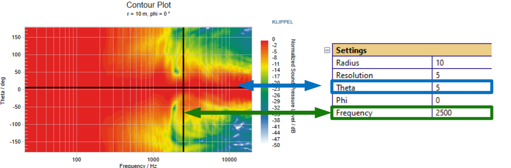
- Display Range Theta
Defines in which unique theta range the contour plot and the beam width plot is mapped.
- Axis Limits Theta and Frequency
Set the visible angular and frequency limits of the contour plot (display only, no data change).
Theta Axis Min: Minimum polar angle (°) shown.
Theta Axis Max: Maximum polar angle (°) shown.
Freq. Axis Min: Lowest frequency (Hz) shown.
Freq. Axis Max: Highest frequency (Hz) shown.
Ideal for zooming into a listening window or critical frequency band.
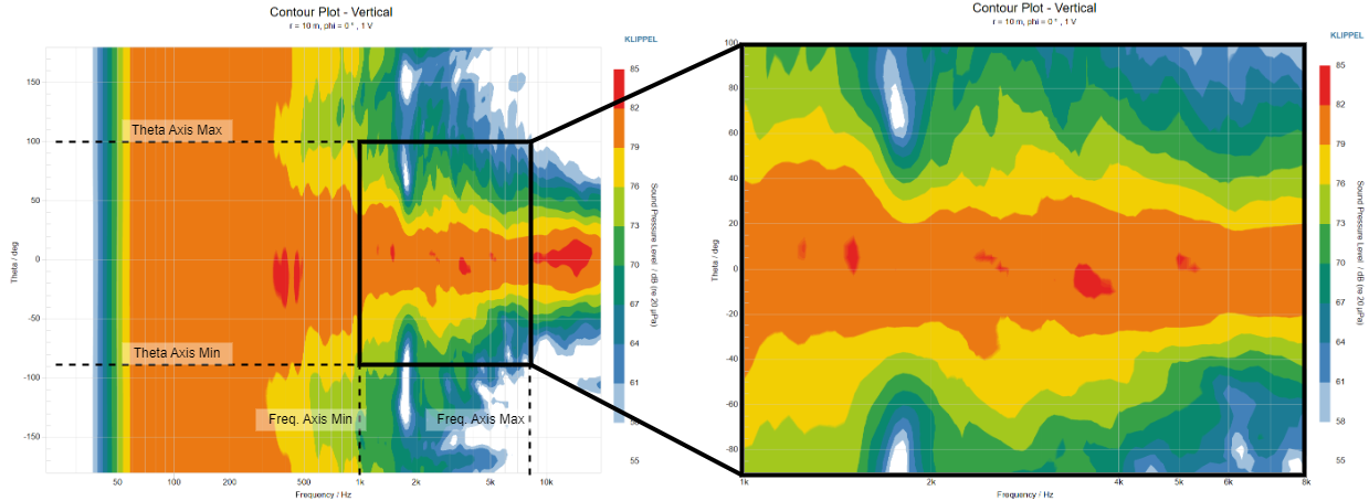
- Show Position Names
Show or hide position tags for Front & Back + Top & Down or Left & Right. Only available for horizontal polar plots (φ={90°,270°} ) and vertical polar plots (φ={0°,180°} )
Beam width#
This category includes display settings of the Beam Width
- Reference Axis
Position to which the beam width plot is referenced this can be the on-axis position or a specified listening point
- Display Range SPL
\(\text{dB}\)
Range of the sound pressure level isobars
- Step Size
\(\text{dB}\)
Increment of the sound pressure level isobars
Polar Plot#
This category includes display settings of the Polar Plot
- Normalize
Polar Plot can be normalized to the maximum sound pressure level
- Display Range SPL
\(\text{dB}\)
Display range of the sound pressure level
- Show Position Names
To simplify the understanding of the Polar Plot, additional position names can be activated that show e.g, which angle is on the left and right of the device under test. Only available for horizontal polar plots (φ={90°,270°} ) and vertical polar plots (φ={0°,180°} )
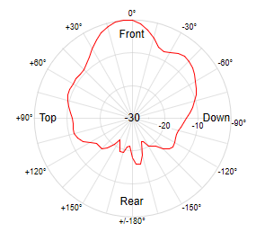
Polarplot vertical 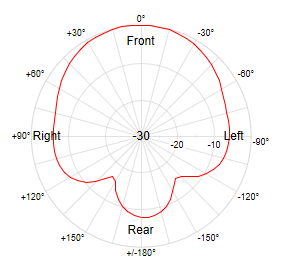
Polarplot horizontal
Directivity Balloon#
This category includes display settings of the Directivity Balloon
- Balloon Type
Selection of the visualization type of the balloon. This can be:
Balloon: SPL is visualized by color and Radius
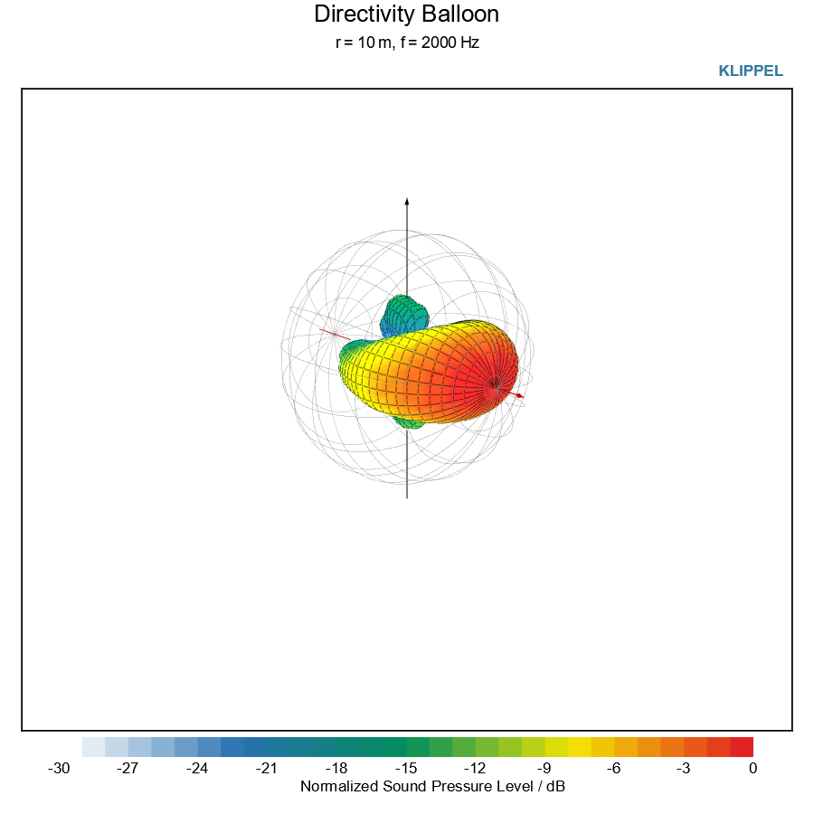
Sphere: SPL is visualized by color, Radius is constant
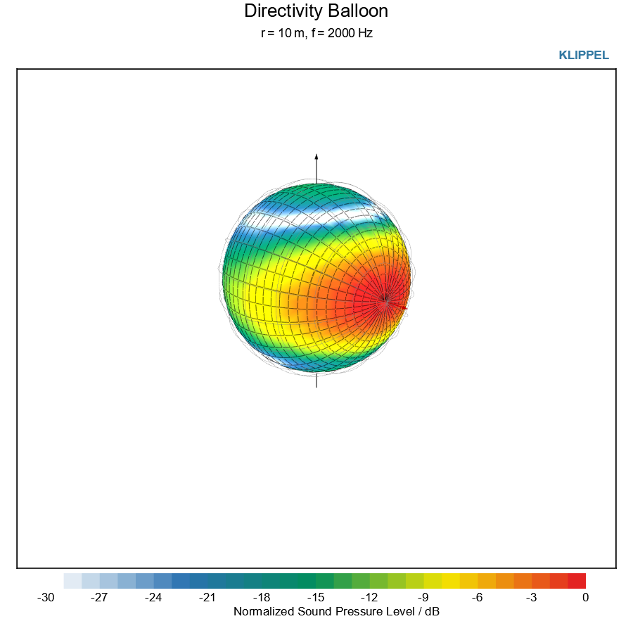
- Color Data
Selection which property should be used for the color coding. This can be:
Sound Pressure level
Phase
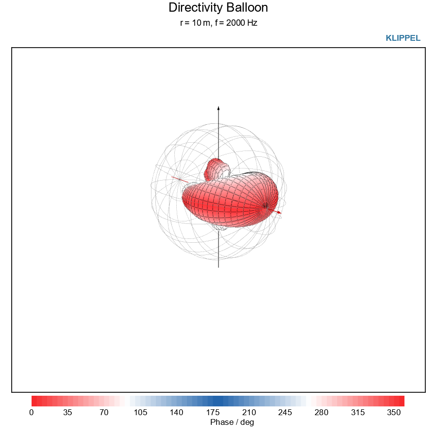
- Normalize
Directivity Balloon can be normalized to the maximum sound pressure level
- Display Range SPL
\(\text{dB}\)
Display range of the sound pressure level
- Color map
The color map of the Directivity Balloon can be defined freely either by using predefined color maps specifying the Display Range SPL + the Color Step Size or by a custom color map. For custom colors any RGB- color matrix can be defined using the following format:
dB SPL  | red (0-255) | green (0-255) | blue (0-255)
dB SPL  | red (0-255) | green (0-255) | blue (0-255)
- Color Step Size
\(\text{dB}\)
Increment of the color map
- Show Mesh
Parameter to show or hide the spherical mesh and the coordinate system
Far Field Data Export#
To use the measurement results of Near Field Scanner for further analysis with external software like EASE or VACS, the Visualization has an export interface for far field data. This tool extracts balloon data in common data formats. The user can define parameters like radius, angle range and resolution freely.
- Export Format
Selection of the export format.
The Visualization support the following Ascii-formats:
VACS (Frequency Response/ Impulse Response)
EASE (Frequency Response/ Impulse Response)
CLF1/CLF2
and binary format:
MATLAB (Frequency Response/ Impulse Response)
SCILAB (Frequency Response/ Impulse Response)
- Curve Format
Selection if the curve data should be exported in frequency domain or in time domain
- Export Phase Data
Frequency Responses can be exported with or without phase information
- Folder
Path to the folder on the hard drive. Here the exported data will be saved.
Coordinates#
This category defines the coordinates, at which the responses are calculated.
The coordinate can be defined freely.
- Radius
\(\text{m}\)
Distance to the Reference Point which corresponds to the spherical radius
- Phi - Minimum
\(\text{°}\)
Minimum value of the circular angle phi
- Phi - Resolution
\(\text{°}\)
Angular resolution of the circular angle phi
- Phi - Maximum
\(\text{°}\)
Maximum value of the circular angle phi
- Theta - Minimum
\(\text{°}\)
Minimum value of the polar angle theta
- Theta - Resolution
\(\text{°}\)
Angular resolution of the polar angle theta
- Theta - Maximum
\(\text{°}\)
Maximum value of the polar angle theta
Processing#
Similar to the far field visualization options, standard signal processing can be also applied to the exported data.
- Reference Voltage
- \(\text{V}\)Per default the Visualization is showing transfer function which are related to 1 Vrms. In order to display the measured SPL output of a device. A reference voltage (e.g. 2.83V) can be defined. All data is scaled linear with this voltage.
- Reference Distance
- \(\text{m}\)To compare data of different devices, it is useful to scale measurement results to a standard distance (e.g. 1 m)Using the 1/r law, this parameter scales magnitude and phase of all graphs to the specified reference distance.
- Result Frequencies
Selection of the displayed frequencies. This can be:
Original (calculated Frequencies of Field Identification)
ISO Frequencies (e.g. R10, R80)
by Resolution (User Defined Resolution in Points per octave)
Custom (User Defined Frequencies)
- Frequency Resolution
\(\text{pts./oct.}\)
Frequency resolution for Result Frequencies setting: by Resolution.
- Custom Frequencies
\(\text{Hz}\)
Table of custom frequencies for Result Frequencies setting: Custom
- Smoothing
\(\text{pts./oct}\)
Parameter to apply a smoothing over frequency to all graphs.
- Remove Time Delay
\(\text{ms}\)
- Parameter to remove a fixed delay from the phase responses. The following
options are available:
Automatic (based on mean group delay)
Distance to Reference Point (propagation delay of the sound wave)
Custom (User defined delay in ms)
Results#
Frequency Response#
The graph show the frequency response (magnitude and phase) of the deivce for a defined position e.g. On-Axis
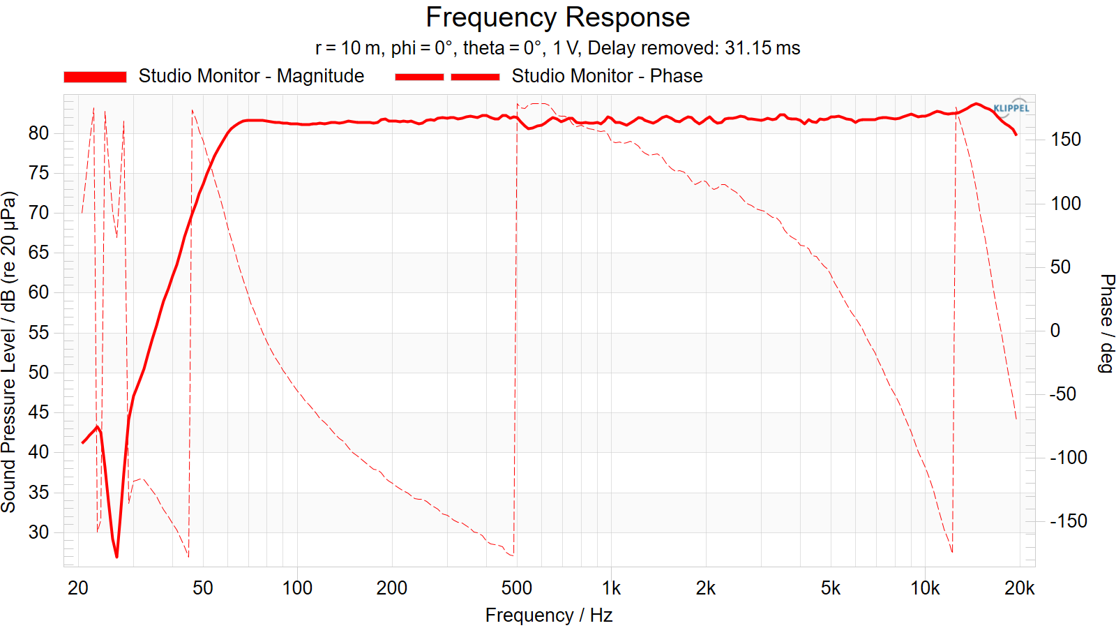
Specified parameters:
Radius
Phi Angle
Theta Angle
Sound Power#
The sound power quantifies the total acoustic energy emitted by a device under test (DUT). It is defined as the integrated sound intensity over the surface area of a sphere surrounding the source.
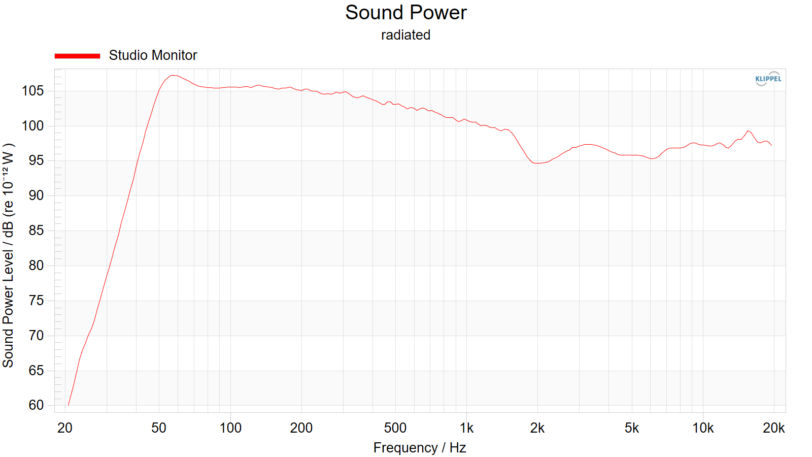
The visualization module employs two distinct calculation methods for determining the sound power:
1. Radiated Sound Power based on holographic coefficients#
Using measurement data from the Near Field Scanner (NFS), the radiated sound power is directly derived from the holographic coefficients. This method considers both full-space (loudspeaker systems measured with the NFS) and half-space (tranducers measured with the NFS Baffle or SCN-NF Addon):
Full space (\(4 \pi\))
\[\Pi(\omega) = \frac{1}{\rho_0 c k^2} \sum_{n=0}^{N} \sum_{m=-n}^{n}\left| {C_{mn}(\omega)} \right|^2\]Half space (\(2 \pi\))
\[\Pi(\omega) = \frac{1}{2 \rho_0 c k^2} \sum_{n=0}^{N} \sum_{m=-n}^{n}\left| {C_{mn}(\omega)} \right|^2\]
Where:
\(\Pi(\omega)\): Radiated sound power
\(\rho_0\): Density of air
\(c\): Speed of sound
\(k\): Wavenumber, defined as \(k = \frac{\omega}{c}\)
\(C_{mn}(\omega)\): Holographic coefficients
2. Integration Over Surface Area#
For Polar Far Field Measurements (POL) and Multi-Source Measurements using the Near Field Scanner (NFS Multi Source Superposition), sound power is calculated by integrating the sound intensity over the surface area of a sphere:
Under far-field conditions, where sound pressure and particle velocity are in phase, this can be expressed as:
Where:
\(I(\omega)\): Sound intensity
\(p(\omega)\): Sound pressure
\(A\): Surface area of the sphere
Sensitivity (microphones only)#
The graph shows the free-field and diffuse-field sensitivity of the microphone being tested.
Note
Analyzing loudspeakers, there isn’t a specific Sensitivity graph. To calculate loudspeaker Sensitivity use the Frequency Response window and scale the graph using the Display Parameter Reference Voltage and Reference Distance (See also Example - Sensitivity:)
Directivity Index#
The directivity index is defined as the ratio between on-axis sound pressure and the sound pressure of all radiation angles.
. 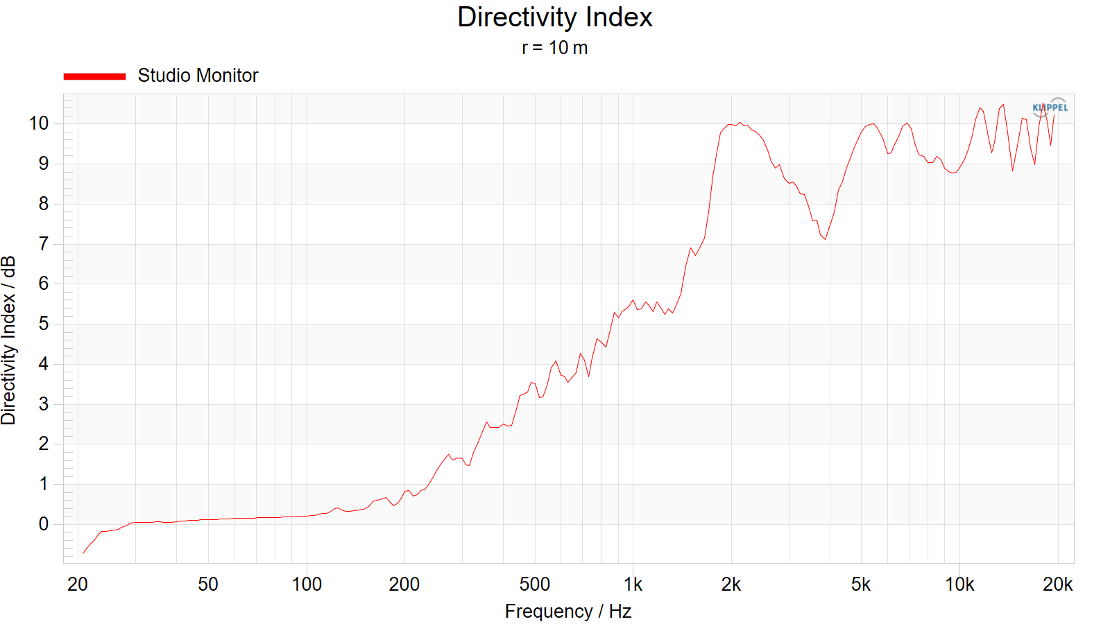
Impulse Response#
Transforming the complex transfer function back into time domain, the Impulse at any point in 3D space can be calculated.
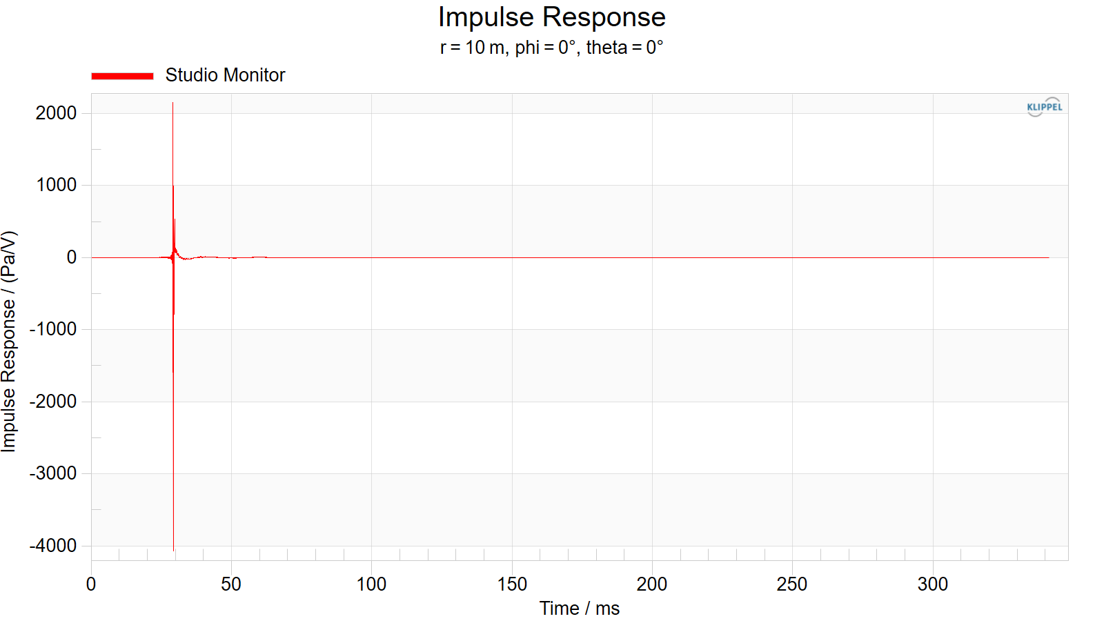
Group Delay#
The group delay is defined as the derivative of the phase response. It shows the propagate time over the full frequency range, which can be used to align loudspeaker systems with multiple transducers.
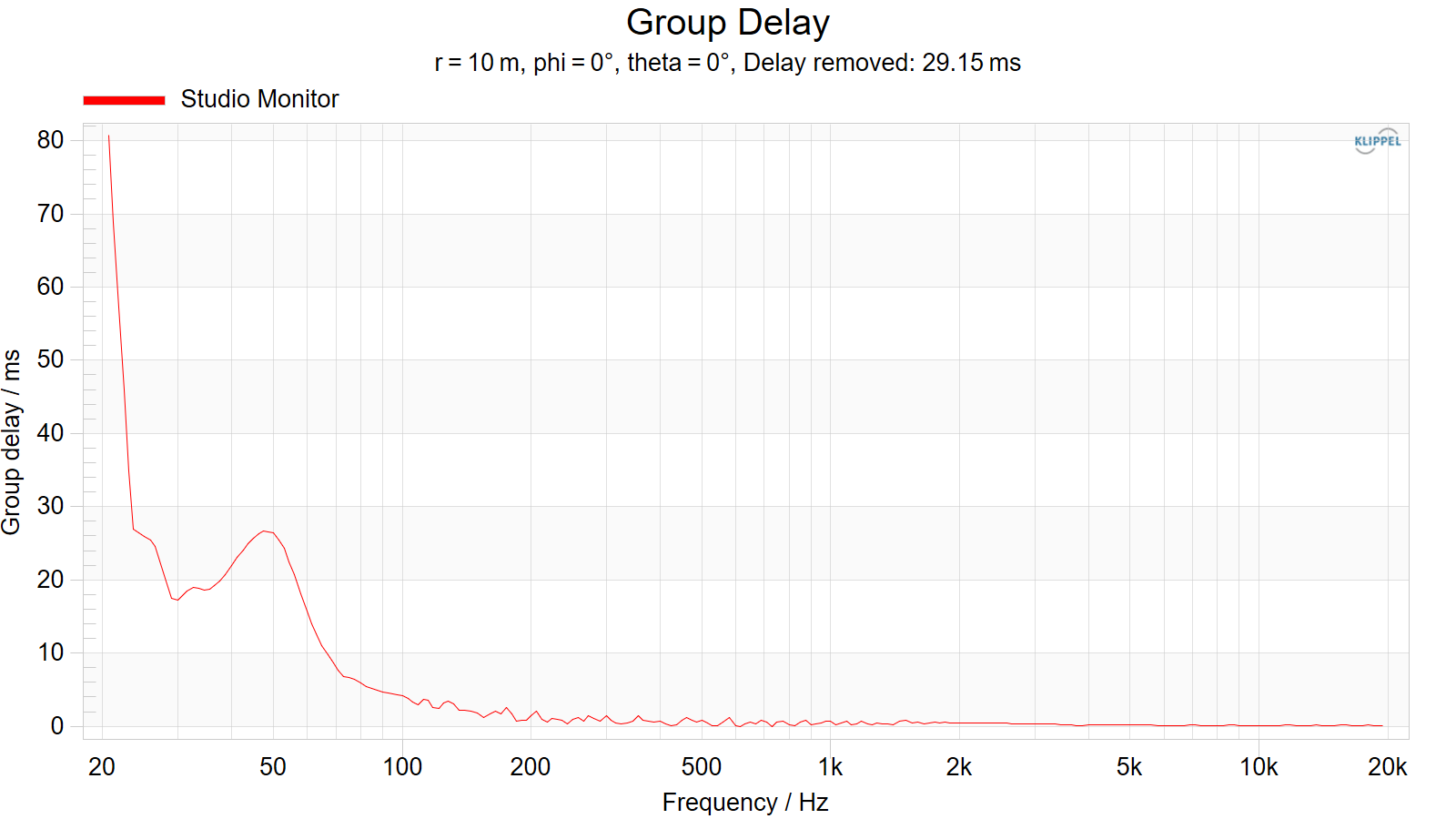
Specified parameters:
Radius
Phi Angle
Theta Angle
Directivity Balloon#
The Balloon plot visualizes directivity pattern over phi and theta for a specified frequency. It shows how much sound is emitted in each direction. The color data can show either sound pressure level or the phase.
Sound Pressure Level
Phase
Specified Parameters:
Radius
Angle Resolution
Frequency
Contour Plot#
The plot provides a directivity analysis over the whole frequency band. It shows very clear how the directivity changes over frequency and at which frequency the first side lobes appear.
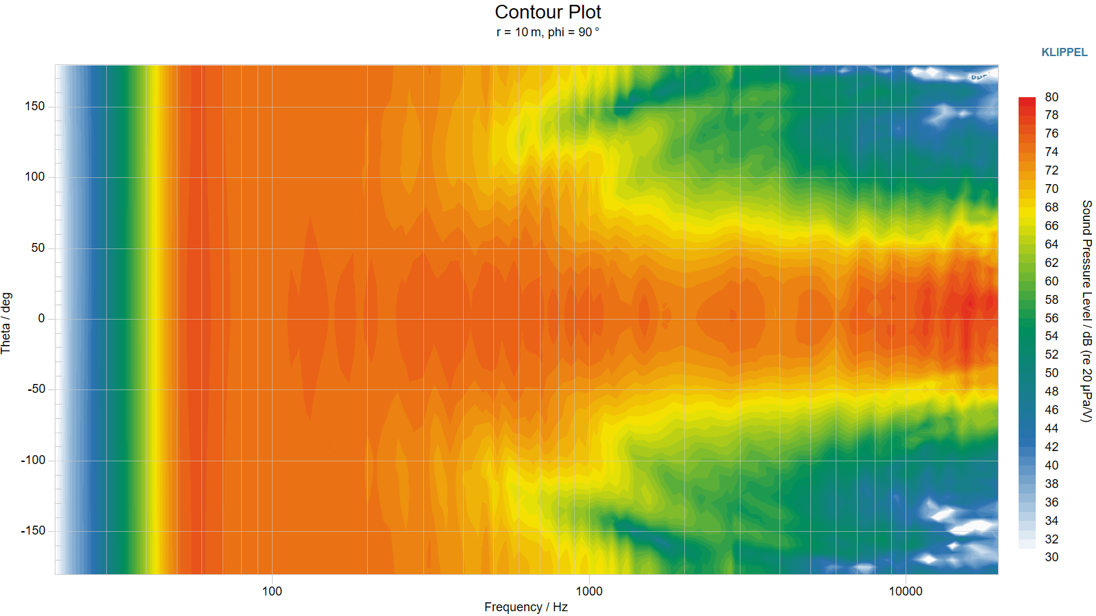
Specified Parameters:
Radius
Angle Resolution
Phi Angle
Beamwidth#
Beamwidth visualizes at which radiation angle the sound pressure level has dropped by a certain value (e.g. 6dB) compared to the On-Axis-SPL.
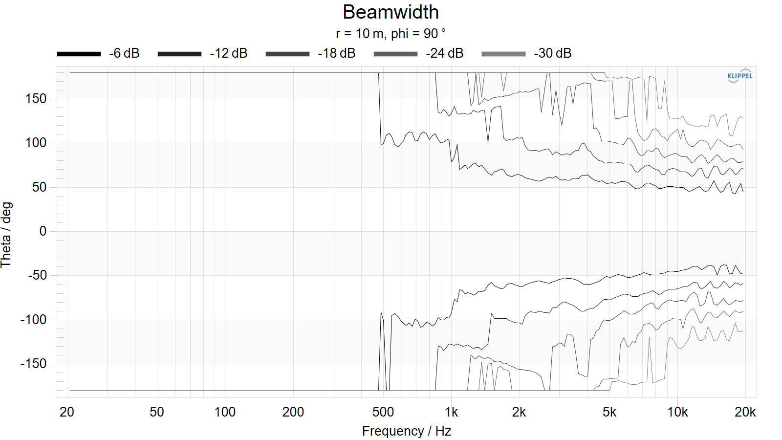
Specified Parameters:
Radius
Angle Resolution
Phi Angle
Polar Plot#
Using a polar coordinate system, the 2D directivity over theta is visualized. This provides a fast analysis of the frequencies with distinct lobes in the directivity pattern.
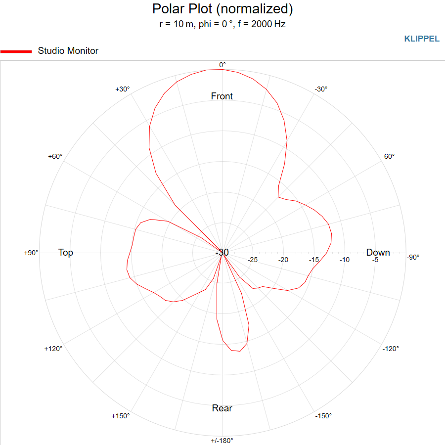
Specified Parameters:
Radius
Angle Resolution
Phi Angle
Near Field – Frequency Response#
The graph shows the transfer functions (magnitude + phase) at chosen positions in the sound field.
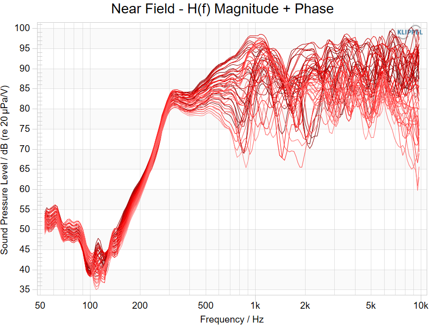
Near Field – Sound Pressure Distribution#
To investigate the sound pressure output in the near field of the device, various projection surfaces can be positioned.
Projection Surfaces#
Cube#
Sphere#
Visualized Data#
The graph is visualizing sound pressure level, phase as well as the sound wave.
Sound Pressure Level#
Phase#
Sound Wave#
Near Field – Configuration#
This window is visualizing the settings of the of the Near Field property page. It shown the projection planes as well as the listening points.
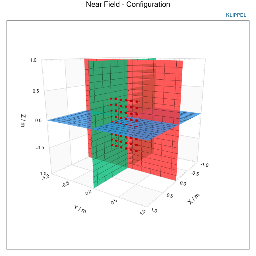
Z(f) Electrical Impedance#
Imported magnitude response of the electrical impedance of the device under test.
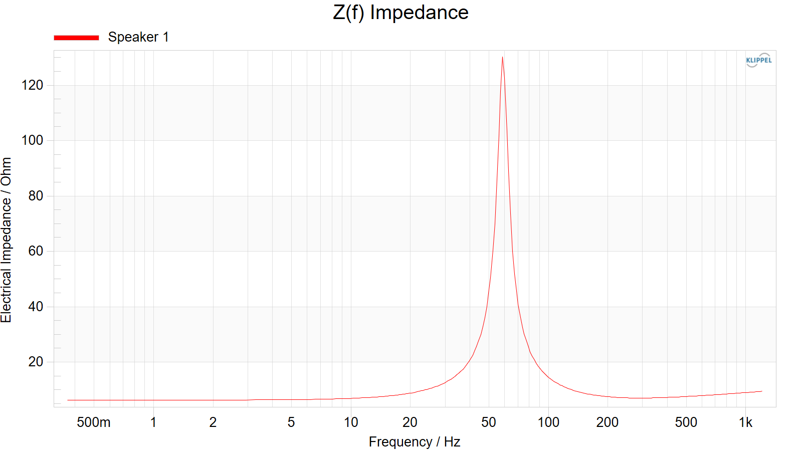
Using the CLF-Data Export this curve will be included automatically into the exported tab-file.
Holographic Parameter Export#
The Holographic Parameter Export Module provides an export of the comprehensive sound field data. Based on this information the sound pressure level at any point outside the scanning surface can be calculated.
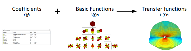
The following data will be exported:
- Sound field coefficients
- \(\mathbf{C}_{nm}(f)\)Coefficients of spherical wave expansion
- Radius of validity
- \(r_{\text{val}}\) in \(\text{m}\)For distances \({r \geq r}_{\text{val}}\) the sound field coefficients are valid
- Expansion point
- \(\mathbf{r}_{\text{ex}}\), \([x,y,z]\) in \(\text{m}\)Expansion point vector with cartesian coordinates
- Reference system
- \(\mathbf{r}_{\text{ref}}\) , \(\mathbf{n}_{\text{ref}}\), \(\mathbf{o}_{\text{ref}}`m :math:`[x,y,z]\) in \(\text{m}\)Reference Point, Reference Axis and Orientation Vector in cartesian coordinates
- Frequency
- \(f\) in \(\text{Hz}\)Frequency vector
The data can be exported in common data format like binaries for MATLAB and SCILAB as well as a plain text ASCII- Format.
Listening Zone#
The Listening zone module is a mini tool to calculate representative curves in a specified listening area.
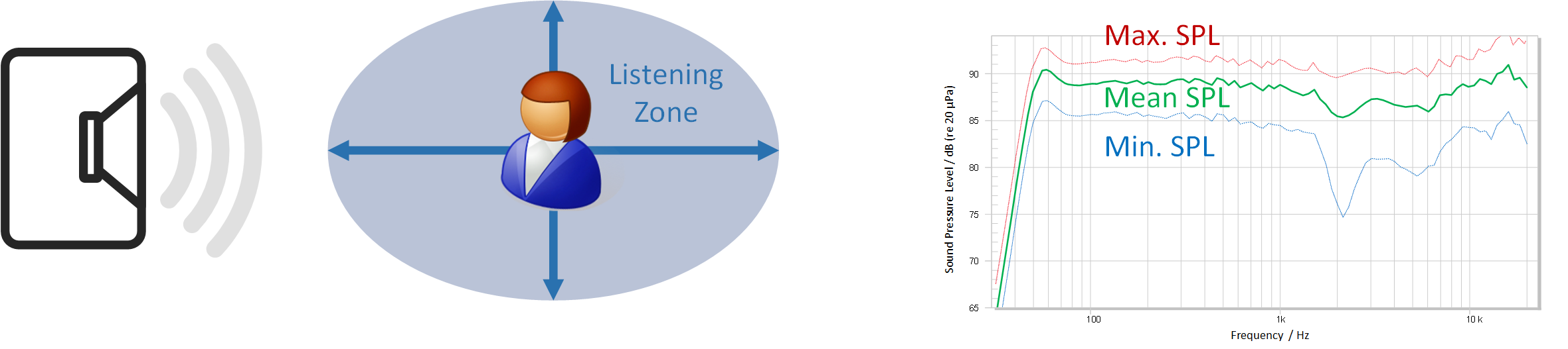
Defining Listening Zones:#
The Configuration parameter of the Property Page can be used to set a single or multiple listening area freely by defining a set of coordinates for each zone.
Surf1_Name = ‘My Listening Zone‘;         // CURVE NAME
Surf1_Coor = ‘sph‘;                       // COORDINATE TYPE: spherical
Surf1_Data =
  [                                         // DATA SECTION:
  <Radius 1> <Phi 1> <Theta 1> <weight 1>   // coordinates of Point 1
  <Radius 2> <Phi 2> <Theta 2> <weight 2>   // coordinates of Point 2
  <Radius 3> <Phi 3> <Theta 3> <weight 3>   // coordinates of Point 3
      :         :       :         :
  ];

// CALCULATION METHOD:
Surf1_Calc = ‘SPL_mean‘;                    // result curve is the mean SPL value of
Surf1_Window = 1;                           // and is plotted to result window 1.

// WINDOW CONFIGURATION
Window1_Title = ’My Summary Window’;        //title of window 1
Window1_Type = ’SPL’;                       //the curve is plotted as a dB SPL value

//DEFINE OTHER CURVES:
Surf2_Name = ’...;
Surf2_Coor = ’...’;
Surf2_Data = [...];
Curve Calculation#
The modules offers several options to summarize for example a cloud of point and transfer functions to some representative output curves. The following calculation modes can be selected.
Power average
SPL average:
Absolute average:
Signal Processing#
- Reference Voltage
- \(\text{V}\)Per default the Visualization is showing transfer function which are related to 1 Vrms. In order to display the measured SPL output of a device. A reference voltage (e.g. 2.83V) can be defined. All graphs are scaled linear with this voltage.
- Reference Distance; Measurement Distance
- \(\text{m}\)To compare data of different devices, it is useful to scale measurement results to a standard distance (e.g. 1 m)Using the 1/r law, this parameter scales magnitude and phase of all graphs to the specified reference distance related to the measurement distance
- Result Frequencies
Selection of the displayed frequencies. This can be:
Original (calculated Frequencies of Field Identification)
ISO Frequencies (e.g. R10, R80)
by Resolution (User Defined Resolution in Points per octave)
Custom (User Defined Frequencies)
- Frequency Resolution
\(\text{pts./oct.}\)
Frequency resolution for Result Frequencies setting: by Resolution.
- Custom Frequencies
\(\text{Hz}\)
Table of custom frequencies for Result Frequencies setting: Custom
- Smoothing
- \(\text{pts./oct.}\)Parameter to apply a smoothing over frequency to all graphs.
CEA 2034 – Spinorama#
A special application of the Listening Zone module is the CEA 2034 Spinorama. The standard defined a set of average curves that characterizes the behavior of a loudspeaker in a normal listening room. To generate these curves, there is a template operation included in the dB-Lab software. In this template, all curves are calculated at 2 m distance. (For templates with other calculation distances please ask KLIPPEL support)
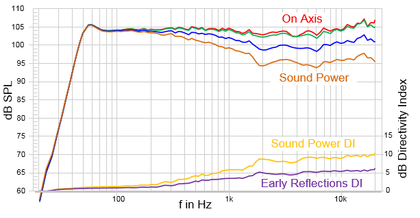
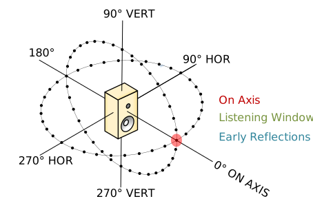
As defined in the CEA2034 standard the results curves \(H_{\text{Res}}(f)\) are calculated by a power average of the specified magnitude responses \(H_{i}(f)\) .
As specified by the standard, the calculation of the Sound Power and the Estimated In-Room Response includes additional weighting factors \(w_i\). These curves are calculated by a weighted power average.
CEA 2034 Summary Window#
The summary window defines the standard reporting format of the loudspeaker. It includes the following curves:
- On Axis
On Axis SPL Response (at theta=0°)
- Listening Window
The listening window curve is a spatial average of the nine magnitude responses in the ±10º vertical and ±30º horizontal angular range.
- Early Reflections
The early reflections curve is an estimate of all single-bounce, first-reflections, in a typical listening room. The definition of the point is shown below.
- Sound Power
The sound power is the weighted rms average of all 70 measurements, with individual measurements weighted according to the portion of the spherical surface that they represent. The weighting values are shown below in the appendix. The weighted power average is calculated.
Note
For half space measurement mode the weights are multiplied by factor 2.
- Sound Power Directivity Index (SPDI)
For the purposes of this standard the Sound Power Directivity Index is defined as the difference between the listening window curve and the sound power curve.
- Early Reflections Directivity Index (EFDI)
The Early Reflections Directivity Index is defined as the difference between the listening window curve and the early reflections curve.
Early Reflections#
The early reflections curve is an estimate of all single-bounce, first-reflections, in a typical listening room. It consists of the following curves:
- Floor Bounce
20º, 30º, 40º down
- Ceiling Bounce
40º, 50º, 60º up
- Front Wall Bounce
0º, ± 10º, ± 20º, ± 30º horizontal
- Side Wall Bounce
± 40º, ± 50º, ± 60º, ± 70º, ± 80º horizontal
- Rear Wall Bounce
180º, ± 90º horizontal
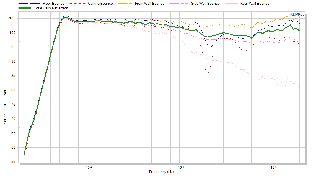
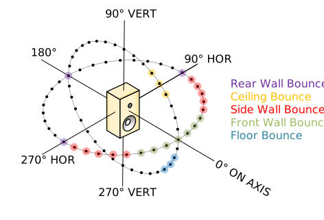
Vertical Reflections#
The window summarizes all reflection which are in the vertical radiation plane.
- Floor Reflection
20º, 30º, 40º down
- Ceiling Reflection
40º, 50º, 60º up
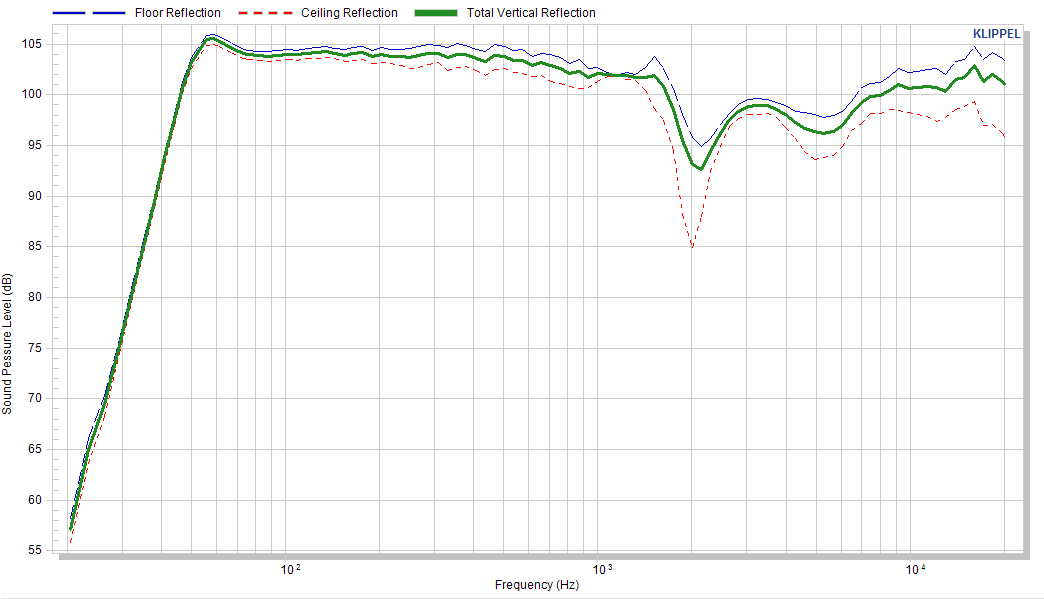
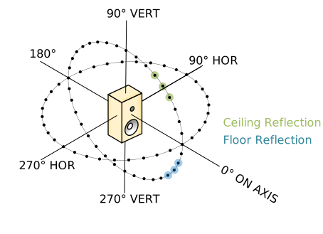
Horizontal Reflections#
The window summarizes all reflection which are in the horizontal radiation plane.
- Front:
0°, ± 10º, ± 20º, ± 30º horizontal
- Side:
± 40°, ± 50°, ± 60°, ± 70°, ± 80° horizontal
- Rear:
± 90°, ± 100°, ± 110°, ± 120°, ± 130°, ± 140°, ± 150°, ± 160°, ± 170°, 180° horizontal, (i.e.: the horizontal part of the rear hemisphere).
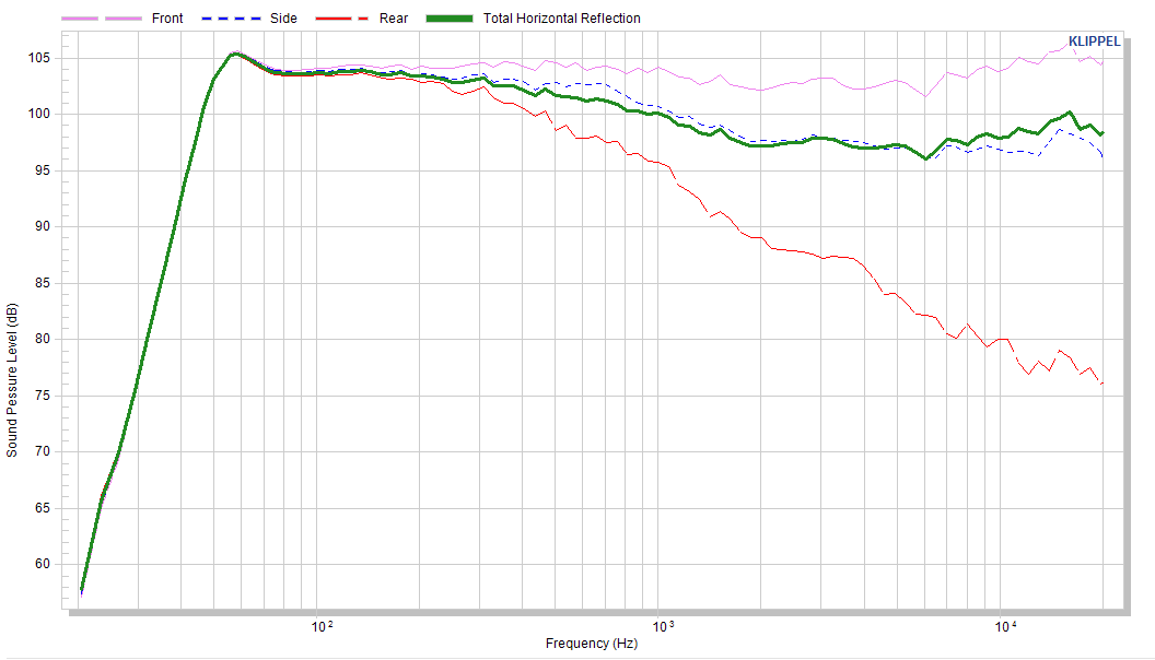
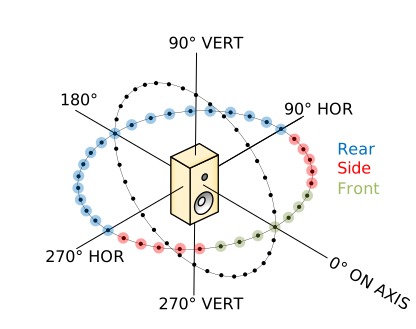
Estimated In-Room Response#
The curve estimates the behavior of the loudspeaker in a normal listen room, It is calculates by using a weighted power average with 12% Listening Window, 44%, Early Reflections and 44% Sound Power.
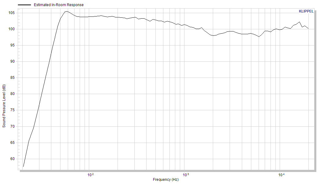
Directivity Index#
Window show the both the Sound power Directivity Index (SPDI) and the Early Reflection Directivity Index (EFDI)
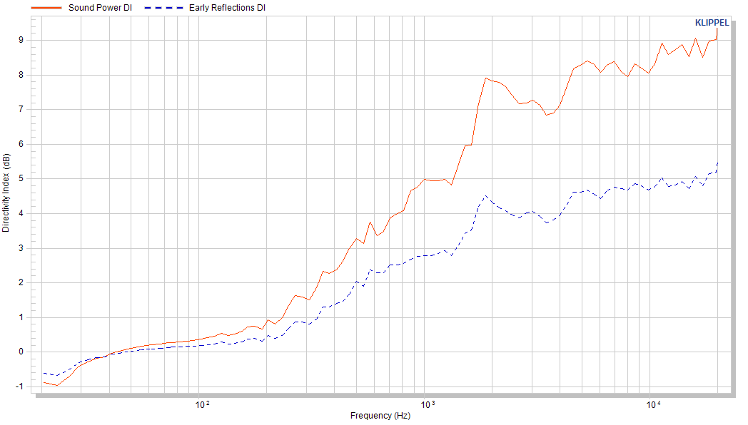
SPL Response Vertical#
The window shows all vertical responses which were are used for the CEA2034 calculation.
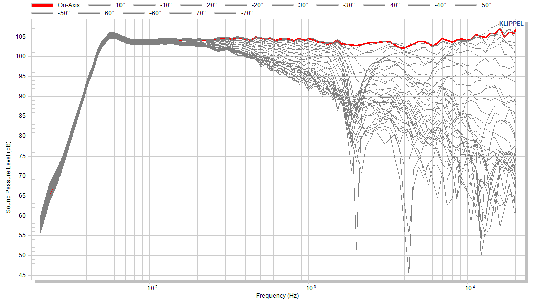
SPL Response Horizontal#
The window shows all horizontal responses which were are used for the CEA2034 calculation.
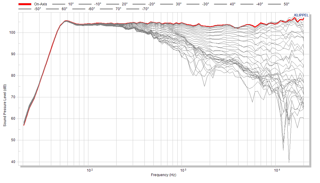
Weighting Table - Sound Power calculation#
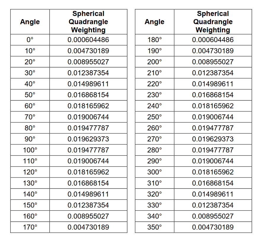
IEC 62777 - Personal Acoustic Zones#
Included in the dB-Lab Software there is an operation template for the IEC 62777 standard that specifies a method to test and evaluate electronic products with directional loudspeaker systems like TV, computer, smart phones or pads. The standard specifies average sound pressure levels in defined personal acoustic zones (e.g. in front, on the sides or at the back of the speaker)
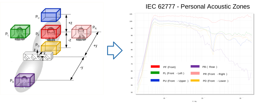
Supported Modules for Im/Export#
Troubleshooting#
Software#
Grid Resolution Warning#
- What happened?
Grid Resolution not high enough. The order is limited and the calculation is done with shown maximum order.
- What to do?
If the Order is insufficient:
Measure more points
Check the Tweeter point
Results might be disturbed by room reflections in certain frequency range#
- What happened?
Reflection free frequency is higher than the upper limit frequency of the field separation. Direct sound cannot be separated from room reflections in the certain midrange frequency band.
- What to do?
Follow the instruction of the output window. There is an advice how the configuration can be changed.
Cannot provide target frequency resolution#
- What happened?
The measured time signal is too short for the desired frequency resolution. For low frequencies the resolution is lower.
- What to do?
If the lower resolution for the very low frequencies is a problem.
Reduce target resolution or
Measure with a longer stimulus.
Not enough measurement points#
- What happened?
The selected order is too high. There are more Coefficients than measured points.
- What to do?
Decrease the order. Measure more points.
Singularity error / not enough independent points#
- What happened?
The Input data is redundant.
- What to do?
Decrease the order. Check the tweeter point.
Memory Allocation error / Stacksize error#
- What happened?
The memory allocation crashes. The program does not get enough memory, which is required for the calculation.
- What to do?
Decrease the order. Reduce Frequency Resolution
Undefined Parameter: …#
- What happened?
A required Input Parameter is not defined.
- What to do?
Open Properties Window and define the Parameter.
